Abstract
As a type of magnetic sensor known for its high reliability and long lifespan, the reliability issues of Hall current sensors have attracted attention in fields such as electromagnetic compatibility. However, there is still a lack of sufficient failure data for reliability prediction. Therefore, a small-sample reliability prediction method based on the improved Bayes method is proposed. Firstly, the pseudo-failure lifespan data are acquired through the accelerated degradation testing of Hall current sensors subjected to temperature and humidity stressors, and the life is examined by the Weibull distribution; then, the data expanded using the BP neural network model are used as the a priori information, and the parameter estimation of the Weibull distribution is obtained by the Bootstrap method and Gibbs sampling; finally, the Peck accelerated model is implemented to achieve the normal temperature-humidity reliability prediction of Hall current sensors under stress, and the utility of the enhanced Bayes technique is confirmed through the application of the Wiener stochastic process model.
1. Introduction
Hall current sensors are magnetic sensors based on the Hall effect that can measure current without contact and are therefore extensively used in many fields such as electromagnetic compatibility, power systems, electronic equipment, speed tests in automotive engineering, etc. [1,2,3]. In practical applications of Hall current sensors, environmental factors will directly affect the service life of Hall current sensors, with temperature and humidity being the two most important and common influencing factors. Prolonged operation of Hall current sensors in high- or low-temperature environments can easily cause phenomena such as core saturation and winding burnout, which in turn lead to measurement errors of the output current. Excessive temperatures also cause wear and tear on the sensor’s sensitive components, which can lead to material aging and electrical failure over time [4,5,6]. Core saturation and winding burnout in Hall-effect devices are two significant issues rooted in distinct physical principles. Core saturation occurs when the magnetic flux in the device’s core exceeds its design limits, usually due to overvoltage or high levels of harmonic distortion. When the core becomes saturated, it cannot effectively channel the magnetic flux, leading to a sharp increase in magnetizing current, which generates excessive heat and can cause thermal damage to the core and surrounding components. Winding burnout, in contrast, is primarily a result of excessive current through the device’s windings. This high current generates heat due to the resistive properties of the winding materials (Joule heating). If the current exceeds the windings’ thermal limits for a prolonged period, the insulation around the windings can degrade and eventually fail. This failure can lead to short circuits between winding turns or phases, resulting in catastrophic damage to the device [7,8]. Additionally, as temperatures rise, the degree of corrosion and aging of the electronic components of Hall current sensors accelerates, and the insulating materials of their circuit boards are decomposed by high temperatures, leading to a decrease in the efficiency of other components. Moreover, if the humidity is too high, it will accelerate the penetration of moisture into the circuit board, making the ion migration phenomenon inside the circuit board more serious, leading to a decrease in the insulation performance of the circuit board, thereby causing the Hall current sensor to be unable to function normally [9]. Therefore, studying the reliability of Hall current sensors is important for ensuring stable operation under various environmental conditions.
Currently, research on product reliability prediction mainly focuses on methods such as failure analysis, neural networks, Monte Carlo (MCS), and stochastic processes. These methods each have their own strengths and weaknesses. Fault analysis methods provide systematic and structured approaches, visualizing fault relationships through graphical and tabular representations, which facilitate the identification and prioritization of critical faults. However, analyzing complex systems can be extremely time-consuming and dependent on specialized knowledge and experience. Additionally, assumptions and data used in these methods may carry uncertainties that affect the accuracy of the analysis results [10,11,12]. Neural network methods in product reliability prediction possess strong self-learning and nonlinear processing capabilities, enabling them to learn complex patterns and relationships from large datasets. They also exhibit strong robustness to noise and incomplete data. However, neural network models are often considered black-box models, lacking interpretability, and their training processes require large amounts of high-quality data and computational resources. Despite their strong predictive capabilities, the complexity of the models and the required training time may pose limitations [13]. Monte Carlo methods are renowned for their flexibility and statistical nature in product reliability prediction and are suitable for handling various complex and high-dimensional problems. They can estimate system behavior and characteristics through random sampling and are widely applied in many fields. However, Monte Carlo methods are computationally expensive, requiring many random samples and computational resources. The precision of the results depends on the sample size, and the convergence speed may be slow. Additionally, the complexity and computational load can become practical obstacles in some cases [14,15]. Stochastic process methods effectively describe the dynamic changes and random behavior of systems in product reliability prediction, making them suitable for addressing time-dependent reliability issues and providing probabilistic descriptions of system failure times. However, constructing and analyzing stochastic process models are complex, relying on precise mathematical models and extensive historical data, and require highly accurate model assumptions. In practical applications, model selection and parameter estimation can be challenging, and computational complexity is also a factor to consider [16]. When using these methods to forecast the dependability of Hall current sensors, an extensive number of samples is needed, and the degradation must follow certain distribution conditions. However, due to the high reliability and long lifespan of Hall current sensors, enough degradation data cannot be obtained within a brief timeframe, making it difficult to apply the above methods to reliability prediction [17].
The Bayes method is commonly used to solve reliability prediction problems for products with small samples. This method can effectively shorten the test period and reduce test costs, so this paper chooses the Bayes method to forecast the dependability of Hall current sensors. First, the Bayesian method can effectively combine prior knowledge with new data, improving prediction accuracy by updating the prior probability distribution. This is particularly important in the case of small samples, where insufficient data may lead to unstable results with traditional statistical methods. Secondly, the Bayesian method can provide probabilistic prediction results, making uncertainty analysis more intuitive and comprehensive. Finally, the Bayesian method excels in handling complex systems and multi-parameter estimation, flexibly adapting to different model requirements, thereby enhancing the accuracy and robustness of reliability predictions [18,19]. When using the Bayes method to predict the reliability of products with small samples, the first step is to collect various prior information based on the characteristics of different products and construct a prior distribution function. Then, integrating sample data with the prior distribution function, the subsequent distribution is obtained. Finally, through two high-dimensional integral operations, the distribution function and estimated value of the parameters are obtained, achieving accurate prediction of product reliability [20,21,22].
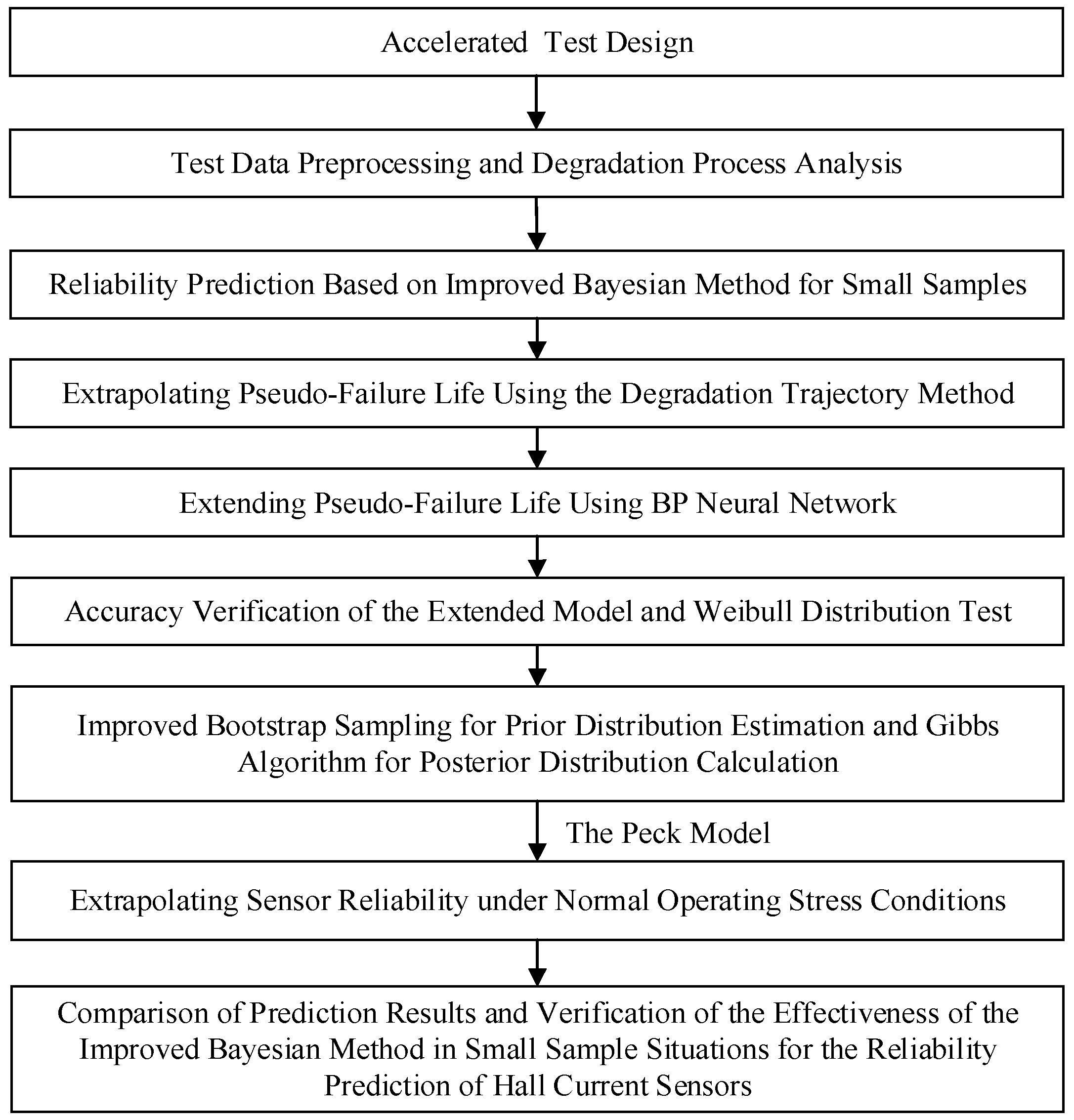
The solution of the posterior distribution based on the Bayes method involves complex and slow high-dimensional integral operations. An improved Bayes method is proposed for the reliability prediction of Hall current sensors with small samples. This method first conducts accelerated test design, experimental data preprocessing, and degradation process analysis. Second, to solve the problem of insufficient prior information for Hall current sensors, a BP neural network model is used to expand small sample data. The BP neural network possesses powerful nonlinear mapping capabilities, as well as self-learning and adaptive abilities. Additionally, the algorithm is relatively simple and easy to implement in programming. Beyond that, a well-trained BP neural network can not only fit the training data well but also accurately predict and classify new input data. Therefore, this model can be used to supplement the prior information of the Hall current sensor to improve the accuracy of predictions. Then, when solving the prior distribution function, an improved Bootstrap method is chosen, which is particularly suitable for analyzing small sample problems. To avoid complex high-dimensional integral operations, the numerical analysis software OpenBUGS3.2.3 is used to program the prior distribution function and prior information, and the Gibbs sampling algorithm is used to solve the posterior distribution parameters, avoiding complex high-dimensional integral operations. Finally, according to the Peck model, the dependability of the Hall current sensor in standard operating circumstances is forecasted, providing a theoretical reference for the service life of the Hall current sensor. The specific process is shown in Figure 1.
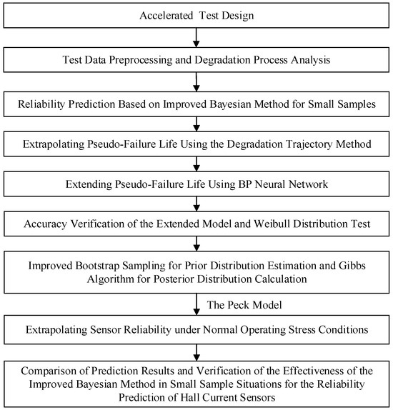
Figure 1.
Experimental Flowchart.
2. Design and Data Analysis of the Acceleration Test Scheme for Hall Current Sensors
2.1. Accelerated Degradation Testing Design
In practical applications of Hall current sensors, environmental factors directly affect the service life of the sensors, with temperature and humidity being the two most predominant and common influencing factors. Therefore, this paper considers temperature and humidity as the accelerated stresses for the sped-up degradation testing of Hall current sensors. Using the sensor’s characteristic parameters and engineering experience, the sensor’s offset voltage (zero-point voltage) is selected as the performance degradation metric for the accelerated degradation testing, with a voltage offset exceeding 10 mV set as the failure threshold. Although considering only the offset voltage to evaluate the reliability of the sensor has its limitations, other parameters can be ignored under certain accuracy requirements. Compared to sensitivity, temperature drift, linearity, and noise level, the offset voltage is the representative and important parameter for evaluating the reliability and service life of Hall current sensors because it directly reflects the health of the sensor’s internal circuitry and materials, serving as an early warning indicator of potential failures. Moreover, measuring the offset voltage is simple and easy, and its changes are usually highly correlated with other performance parameters, indirectly reflecting the overall health of the sensor. As a key measurement parameter widely recognized by industry standards, the offset voltage excels in stability and data repeatability, making it the preferred parameter in reliability evaluations. By monitoring the offset voltage, the analysis process and models can be simplified, reducing complexity and computational load, thereby providing sufficient reliability information when resources are limited or quick assessments are needed. When setting the stress levels of temperature and humidity, two issues must be considered. First, the stress levels of temperature and humidity should accelerate the failure process of the Hall current sensor without altering its failure mechanism [23,24,25,26]. This means that the selected maximum temperature should not exceed the sensor’s limit temperature under normal working conditions. The maximum operating temperature of the Hall current sensor is 85 °C; therefore, the maximum test temperature level (Tmax) is chosen to be 80 °C. The highest temperature during normal operation of the Hall current sensor is around 40 °C. If the test temperature level is too low, it will lead to an extended test duration. Therefore, the minimum temperature level (Tmin) is set to 50 °C. According to the sensor’s characteristic parameter table, its operating humidity without condensation is 20% to 90% RH. Hence, the maximum test humidity (RHmax) is chosen to be 80% RH, and the minimum test humidity (RHmin) is set to 60% RH. Additionally, the number of accelerated stress levels should be at least three. However, due to test cost and time constraints, this test will select three groups of temperature and humidity stress level combinations. To ensure appropriate intervals between the selected temperature and humidity stress levels, the intermediate temperature level (Tmid) and humidity level (RHmid) are selected as 65 °C and 70% RH, respectively.
Considering the comprehensive national standard IEC 60068-2-78 [26] and the cost of testing, a random sample of 24 Hall current sensors from the same batch of products is selected as the test specimens. The quantity of samples tested at each stress level is eight. The number of test cycles for the sensors under different stress groups is 15, with each cycle lasting 24 h, totaling 360 h. The accelerated degradation testing of the Hall current sensors is conducted on the acceleration platform shown in Figure 2. The required accelerated test equipment mainly consists of a constant temperature and humidity chamber, Hall current sensors, a multifunctional calibrator, a DC stable voltage and current power supply, and a Hall current sensor zero-voltage detection device. Standards such as IEC 60068-2-78 and JEDEC JESD22-A101 primarily focus on testing conditions in humid and hot environments and do not specify requirements for electromagnetic shielding [23,24,25,26]. However, to prevent external electromagnetic interference from affecting the sensor test results, it is generally recommended that the test environment be kept as free from strong electromagnetic interference sources as possible. Therefore, the experimental platform in this study is set up in a shielded room, and the testing equipment employs shielded cables and proper grounding to avoid electromagnetic interference. Additionally, the background magnetic field strength of the test chamber used in this study was measured to be 19 nT. The Hall sensor used in this study has a rated current of 6 A, and the test current was set to the rated value. The calculated magnetic field strength generated by the sensor is approximately 0.24 mT. Therefore, the 19 nT magnetic field strength in the chamber can be considered negligible.
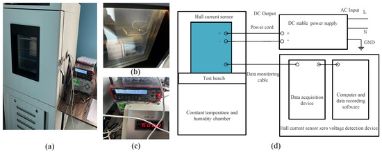
Figure 2.
Picture and block diagram of the acceleration test platform. (a) Constant temperature and humidity chamber. (b) Hall current sensors. (c) DC stable power supply and Hall current sensor zero-voltage detection device. (d) Block diagram of the acceleration test platform.
2.2. Degradation Data Processing and Analysis
After obtaining the degradation data of the Hall current sensor samples under various stress conditions according to the accelerated degradation testing plan, it is essential to examine and manipulate the data to comprehend the degradation trends of the zero-point voltage in Hall current sensors under varying stress conditions. Common data optimization algorithms include Kalman Filtering, Particle Filtering, Adaptive Filtering, Ensemble Methods, Bayesian Model Averaging, Time Series Analysis, Autoregressive Integrated Moving Average models, machine learning, and deep learning algorithms. Compared to other data processing methods, the advantage of using the improved data fusion method with weighted data points lies in its ability to more effectively utilize the information from each data point. By assigning different weights to different data points, reflecting their importance and reliability, the overall prediction accuracy is improved. Additionally, the weighted data fusion method can reduce the impact of noise and outliers on the results, enhancing the stability and robustness of the model [27,28,29,30,31,32]. Compared to simple averaging or indiscriminate data processing methods, weighted data fusion can more accurately capture key patterns and trends in the data, making it particularly suitable for the integration of complex systems and multi-source data. Therefore, this paper adopts an improved data fusion method, assigning different weights to the five data points x1, x2, …, x5 measured for each sample in each cycle. When the test data deviate less from the average test value, a larger weight is assigned, and conversely, a smaller weight is assigned, thereby improving the accuracy of data fusion. The specific steps are as follows:
First, calculate the average of the data points:
Secondly, calculate the deviation di of each data point from the average:
Then, assign different weights according to the magnitude of the deviation. Data with smaller deviations should be given larger weights, while data with larger deviations should be given smaller weights. The method for calculating the weights is as follows:
In the Formula, wi represents the weight of each data point, and is a very small positive number used to prevent the denominator from being zero.
Finally, complete the calculation of the weighted average of the data.
In the Formula, is the result after data processing.
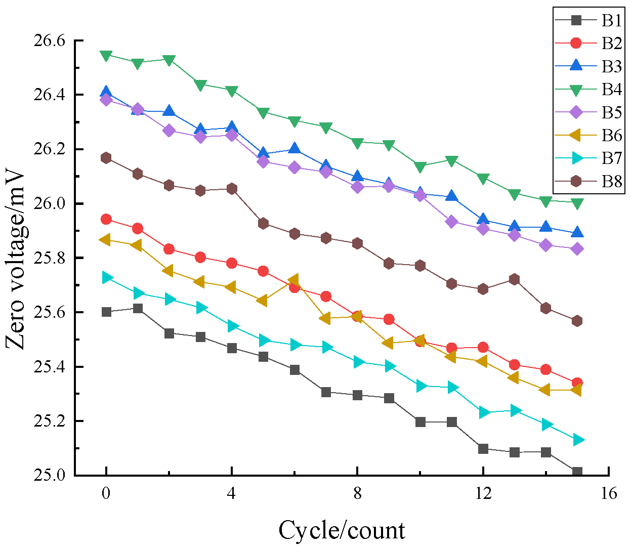
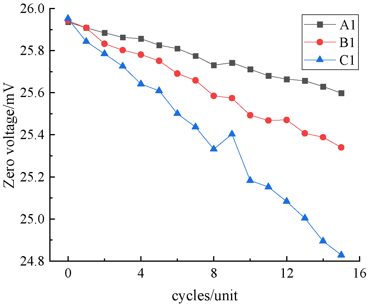
After processing the degradation data under all stress combinations using this method, the degradation curves of the zero-point voltage at 65 °C-0%RH are presented as an example in Figure 3. At the same time, to clearly compare the degradation rates of the zero-point voltage across various temperature and humidity stress levels, the degradation curves of three samples, 50 °C-60%RH-A1, 65 °C-70%RH-B1, and 80 °C-80%RH-C1, are plotted together in Figure 4.
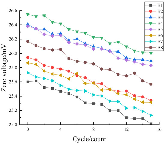
Figure 3.
Zero-point voltage degradation curves under 65 °C-70%RH stress.
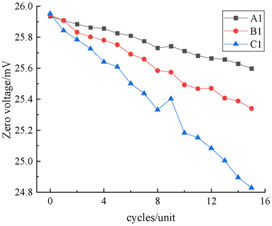
Figure 4.
Variation of zero-point voltage under different stresses.
As is evident from Figure 3, the degradation curves of the zero-point voltage for the eight sensor samples under this stress are quite similar and show a linear decrease. From Figure 4, it is evident that the degradation rate of the zero-point voltage of the Hall current sensors under 80 °C-80%RH stress is significantly higher than that under other temperature and humidity stress combinations. An increase in the temperature and humidity stress combination corresponds to a more rapid degradation pace of the zero-point voltage, leading to a decrease in the performance and accuracy of the Hall current sensor.
3. Hall Current Sensor Prior Information Processing
3.1. Extrapolated Pseudo-Failure Life
To obtain the pseudo-failure lifespans for various Hall current sensor samples, it is necessary to first fit the degradation data of the sensors to obtain the most suitable degradation curve model. Taking the degradation curves of the three samples, 50 °C-60%RH-A1, 65 °C-70%RH-B1, and 80 °C-80%RH-C1, as examples, this section details the specific process for calculating the pseudo-failure lifespans. The degradation data are fitted with linear, power, exponential, and logarithmic models using the least squares method, and the optimal fitting function is selected based on the sum of squared residuals (SSE) and the correlation coefficient (R2). The fitting results are shown in Table 1.

Table 1.
SSE and R2 after fitting the sample data to each mathematical model.
As shown in Table 1, for the three samples, the sum of squared residuals (SSE) is the smallest and the R2 value is close to 1 under the linear model fitting. Therefore, it can be considered that the performance degradation amount and zero-point voltage of the Hall current sensor will decrease linearly with the extension of the usage cycle. Using the linear fitting results in combination with the failure criterion, the pseudo-failure lifespan of the Hall current sensor samples under various stress conditions is extrapolated. Table 2 gives the pseudo-failure lifespan of eight Hall current sensor samples under the 65 °C-70%RH stress combination.

Table 2.
Pseudo-failure lifespan for specimens subjected to 65 °C-70%RH stress conditions.
3.2. Pseudo-Failure Life Distribution Test
The Weibull distribution has good compatibility and can fit various types of data, describing the failure process of products at different stages. When utilizing the Weibull distribution to represent the pseudo-failure lifespan of Hall current sensors, it is essential to initially assess whether the pseudo-failure lifespan data of the sensors follow a Weibull distribution. The Anderson-Darling test method is chosen to test the distribution to which the pseudo-failure life of Hall current sensors adheres, and the distribution test results are shown in Table 3.

Table 3.
Distributional hypothesis Anderson-Darling test results.
In Table 3, a value of H (Hypothesis Test Result) equal to 0 indicates acceptance of the distribution hypothesis, whereas a non-zero value indicates rejection of the distribution hypothesis; P represents the test values for each distribution, indicating the probability of conforming to the distribution; AD* is the statistic for the Anderson-Darling test; and the critical value CV is a standard used to determine whether the AD* is greater than this value. If the AD* is greater than the CV, we can reject the null hypothesis, meaning that the data do not conform to the specified distribution. As seen from the Anderson-Darling test results in Table 3, the pseudo-failure lifespan data of the Hall current sensors conform to all three hypothesized distributions, but the probability of conforming to the Weibull distribution is the highest. Therefore, the Weibull distribution can be considered as the most suitable distribution function for the pseudo-failure lifespan of Hall current sensors.
3.3. Pseudo-Failure Life Expansion
When using the Bayes method to analyze product reliability, it is usually necessary to have a large amount of failure data to construct a failure distribution model. When the number of test samples is insufficient, it is necessary to use the sample expansion method to expand the prior information. The BP neural network model, as a commonly used sample expansion model, has a simple prediction process and highly accurate results. When performing pseudo-failure life extension in cases where the original data may not adequately represent the full range of potential degradation behaviors, neural network models may face issues such as insufficient representativeness of training data and overfitting, leading to decreased accuracy in predicting unseen degradation behaviors. To address these issues, data augmentation, transfer learning, cross-validation, and regularization techniques can be employed to enhance the model’s generalization ability. Additionally, ensemble learning methods can improve prediction stability and accuracy, while regularly monitoring and updating the model helps to continuously improve its performance. These measures can effectively mitigate the limitations and biases caused by insufficient data representation, thereby enhancing the accuracy and reliability of predictions. Therefore, the BP neural network model is chosen to expand the pseudo-failure lifespan data of the Hall current sensor, and the expanded pseudo-failure life data are used as prior information. The BP neural network structure adopted in this paper includes an input layer, a hidden layer, and an output layer. The input layer processes eight input samples, the hidden layer contains 10 neurons and uses the tansig (tangent sigmoid) activation function, while the output layer processes eight output samples and uses the purelin (linear) activation function. The expansion of the pseudo-failure lifespan of the Hall current sensor at 65 °C-70%RH is taken as an example.
Firstly, it is essential to provide the BP network with original input and output data pairs for network training. Using empirical reliability as the input during BP neural network learning and the original pseudo-failure life data as the output during BP neural network learning, the training of the BP neural network is completed. The original data are obtained by performing a weighted average on the accelerated test data by (1) to (4). In cases where the sample distribution model of the data is unknown, the empirical distribution function can be used as an input to the BP neural network to estimate empirical reliability. However, when the sample distribution model is known and the sample size is small, the empirical distribution function may have significant computational errors. To reduce the error in the case of small samples and improve the prediction effect, the mathematical expectation formula can be used to calculate the empirical reliability.
Within the Equation, n denotes the count of samples, while N signifies the number of augmented samples. The empirical reliability of the eight sensor samples is calculated as follows.
After training is completed, the training results are verified for accuracy against the original data, as shown in Table 4.

Table 4.
Model Accuracy Check.
As shown in Table 4, the forecasting precision of the BP neural network is extremely high, with the absolute value of the relative discrepancy between the forecasted values and the original data being under 1%. This indicates that the BP neural network model has been successfully trained.
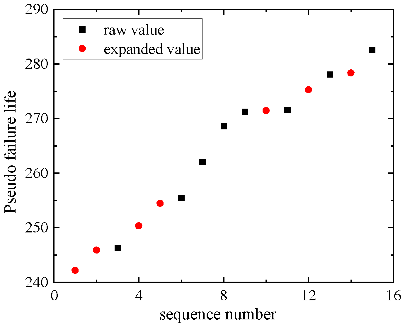
After training is completed, the random empirical reliability R(ti) = {0.85, 0.8, 0.77, 0.7, 0.6, 0.55, 0.35} is input into the trained BP neural network to complete the expansion of the pseudo-failure lifespan data. The seven expanded data obtained are {254.47, 245.91, 242.20, 275.29, 278.34, 271.46, 250.34}.
To determine the fit between the original pseudo-failure life data and the expanded data, a comparison result graph of the original sample’s pseudo-failure life data and the expanded data is provided, as shown in Figure 5.
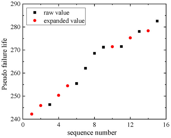
Figure 5.
Comparison results between original and expanded data.
4. Improved Bayes Method for Solving Weibull Distribution Parameters
4.1. Solving for the Prior Distribution
Taking the pseudo-failure lifespan of the 15 samples acquired from the expansion under the 65 °C-70%RH stress combination as the prior information for the Hall current sensor, remove one sample at a time in order, and fit the remaining 14 sensor samples’ pseudo-failure life data to the Weibull distribution. Take the average of the 15 sets of magnitude parameters α and shape parameters β obtained and substitute the results into the Weibull empirical distribution function.
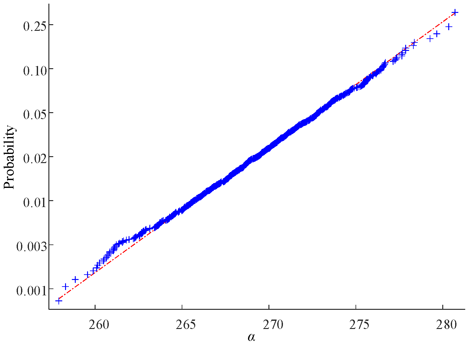
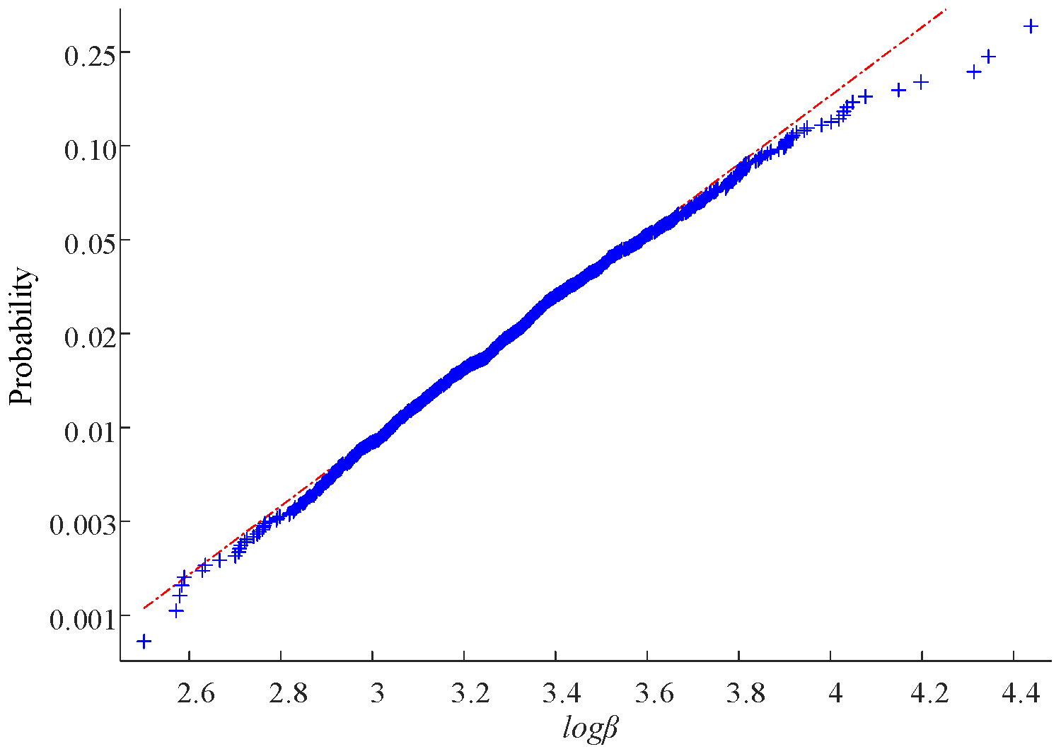
Using the Bootstrap method, randomly extract 1500 samples from the empirical distribution function, group them in sets of 15 samples, and perform Weibull distribution fitting to obtain 1500 sets of estimates for α and β. After removing the first and last 50 sets of parameter estimates, the distribution function fitting is performed to ultimately obtain the prior distribution for α and β under 65 °C-70%RH stress.
Using the distribution test scatter plot to test the distribution of the two parameters, the results indicate that α and β follow the normal distribution and log-normal distribution, respectively. Figure 6 and Figure 7 show the normal distribution and log-normal distribution test results for α and β at a confidence level of 95%, respectively.
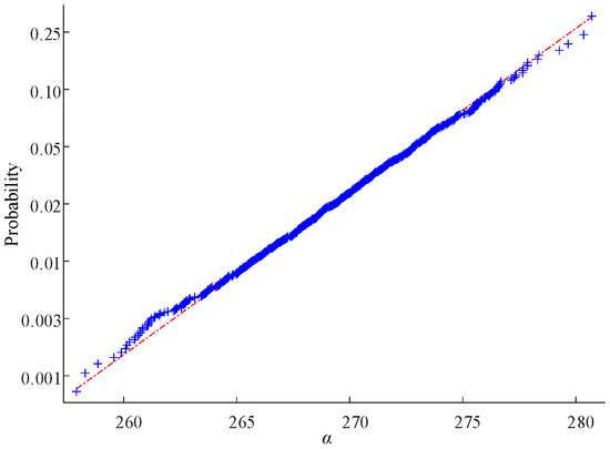
Figure 6.
Scatterplot of α distribution test.
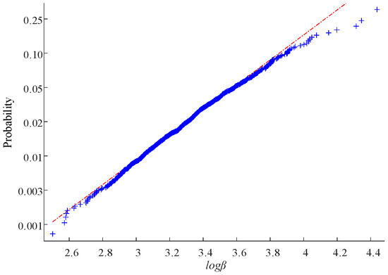
Figure 7.
Scatterplot of β distribution test.
4.2. Calculating the Posterior Distribution
To avoid complex high-dimensional integral operations in the posterior distribution of Hall current sensors, the OpenBUGS software, which incorporates the Gibbs numerical simulation algorithm, is chosen to solve for the posterior distribution of Hall current sensors. The basic steps are as follows. First, program the prior distributions of α and β using the BUGS language; second, check the code for correctness and load the original pseudo-failure life data of the Hall current sensors; then, set the parameters that need to be monitored, and configure the number of Markov chain iterations, the count of iterations, and the count of burn-in iterations; finally, output the statistical parameters of the subsequent distribution of the sample parameters after the iteration has stabilized, including MC error, mean, quantiles, and other parameters, and select the mean as the estimate of the Weibull distribution parameters to forecast the dependability of the Hall current sensors. According to the above steps, set the number of iterations to 60,000, and the number of burn-in iterations to the first 1,000, the results of which are presented in Table 5 and Table 6.

Table 5.
The a posteriori statistic for the parameter α.

Table 6.
The a posteriori statistic for the parameter β.
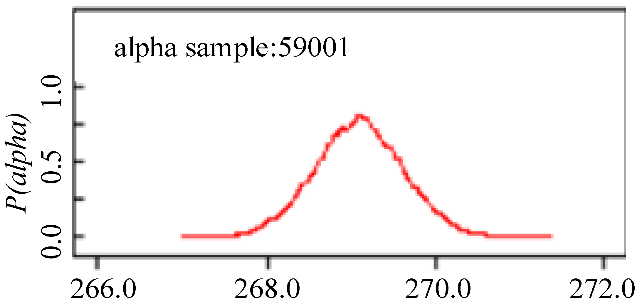
As can be seen from Table 5 and Table 6, the more iterations there are, the more stable the mean values of α and β become, and the error of the MC sampling is gradually decreasing. The posterior probability density of α and β after 60,000 iterations is shown in Figure 8 and Figure 9.
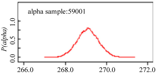
Figure 8.
α a posteriori distribution density.
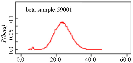
Figure 9.
β a posteriori distribution density.
The point estimates of the Hall current sensor parameters are determined to be the mean of the parameter posterior statistics. Combining Table 5 and Table 6, as well as Figure 8 and Figure 9, after 60,000 iterations, the α and β of the Weibull distribution for the Hall current sensor under the 65 °C-70%RH stress are 269.1 and 23.11, respectively.
Similarly, the improved Bayes method is used to solve for the Weibull distribution parameters of the Hall current sensor under the 50 °C-60%RH and 80 °C-80%RH stresses. The point estimates of the magnitude and shape parameters under each acceleration stress are obtained, as shown in Table 7, which are used to evaluate the dependability and service life of the Hall current sensor in standard operating circumstances.

Table 7.
Parameter estimation results for different stress combinations.
5. Reliability Prediction of Hall Current Sensors under Normal Stress Levels
In practical engineering, in order to assess and predict the reliability of products under normal working stress levels through accelerated testing techniques, it is necessary to ensure that the product’s failure mechanism remains unchanged under different applied stresses. The consensus for validating the consistency of accelerated failure mechanisms in the Weibull distribution model is that the magnitude parameter is a function of the accelerated stress, while the shape parameter is constant. By comparing and analyzing the Weibull distribution parameters of the pseudo-failure lifespan of Hall current sensors under different stress levels in Table 7, it can be observed that the magnitude parameter varies significantly under different accelerated stresses, while the shape parameter exhibits a small variation and good consistency. From this analysis, it can be concluded that the failure mechanism of the Hall current sensors did not change under the three accelerated stress levels.
When the pseudo-failure lifespan of Hall current sensors follows a Weibull distribution, their dependability function can be expressed as (12).
Since temperature and humidity are the main factors affecting the performance degradation of Hall current sensors, the Peck model is selected to depict the correlation between the degradation rate of Hall current sensors and the temperature and humidity stress levels.
where R is a parameter related to the rate of performance degradation, T is the temperature, and RH is the relative humidity.
Based on the estimated values of the Weibull magnitude parameters under different stress combinations in Table 7, the global optimization algorithm is used to fit the parameters a1, b1, and c1 in the Peck model. The relationship between the magnitude parameter and the temperature and humidity acceleration stress is obtained, as shown in (14).
By substituting the normal operating environment temperature (25 °C) and humidity (40%RH) of the Hall current sensor into (14), the estimated value of the magnitude parameter under normal temperature and humidity levels is obtained as 3005.37. In accordance with the principle of consistency of accelerated failure mechanisms, the shape parameter can be represented by the mean of the shape parameters obtained under each accelerated stress, thereby obtaining a shape parameter of 23.47 for the Hall current sensor under normal stress levels.
Consequently, the reliability function of the Hall current sensor under normal temperature and humidity stress levels can be expressed by (15).
Based on the above equation, the dependability curve of the Hall current sensor under normal temperature and humidity stress levels can be acquired. Since it is difficult to verify the reliability prediction results of the improved Bayes method using actual service life information, this paper chooses to use the Wiener stochastic process model to validate the effectiveness of the proposed improved Bayes method.
The comparison of reliability curves for the two methods is shown in Figure 10.
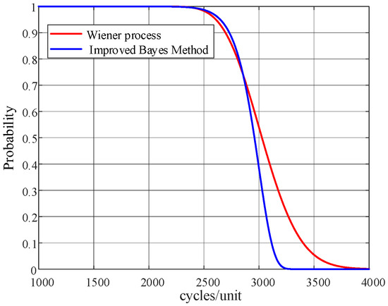
Figure 10.
Comparison of Reliability Curves for Two Methods.
As shown in Figure 10, the reliability curves obtained by the two prediction methods exhibit the same overall trend, but there are some differences. The main reason for these differences is that while the Wiener model considers the randomness in the sensor’s performance degradation process, the limited number of sensor samples used in the accelerated degradation tests does not effectively capture the randomness and variability of the performance degradation parameters during the degradation process. Overall, the reliability forecasting outcomes derived from the enhanced Bayes approach and the Wiener process are fairly similar. Additionally, since the BP neural network model in the improved Bayes method can expand small-sample degradation data, it can still be used when the number of test samples is small. Compared to the Wiener stochastic process, this method has a wider range of applicability and is more advantageous in handling reliability prediction problems with small samples. In practical engineering applications, there is no strict regulation for the service life of Hall current sensors, and the manufacturer’s recommended service life is 6–8 years. The variation in reliability thresholds can significantly affect the estimated service life of Hall current sensors. Increasing the threshold (e.g., from 0.9 to 0.95) will shorten the estimated service life but increase reliability, whereas decreasing the threshold (e.g., from 0.9 to 0.85) will extend the estimated service life but increase the risk of failure. The sensitivity of reliability thresholds can be evaluated through sensitivity analysis, observing the impact of different thresholds on service life estimation. High-quality data and accurate models can reduce the uncertainty of service life estimation due to changes in thresholds. Therefore, the appropriate selection of reliability thresholds is crucial to balance product quality, cost, and failure risk. In this example, reliability thresholds of 0.8, 0.85, 0.9, and 0.95 are used to estimate the service life of Hall current sensors based on Figure 10, with the results shown in Table 8. As indicated in Table 8, the estimated service lives based on these thresholds all fall within the range of 6–8 years. It is generally accepted that Hall current sensors are not suitable for continued operation when their reliability drops to 0.9. According to Figure 10, the service life of the Hall current sensor under normal temperature and humidity stress conditions is defined as the time when the sensor’s reliability reaches 0.9, which is 2725 days, or approximately 7.5 years.

Table 8.
Service life estimation of Hall current sensors under different reliability thresholds.
6. Conclusions
In response to the lack of sufficient failure data for Hall current sensors, this paper makes full use of the experimental data obtained from accelerated degradation tests and adopts an improved Bayes method to forecast the dependability of Hall current sensors under small sample conditions, obtaining the service life of the sensors under normal temperature and humidity stress levels. At the same time, the stochastic Wiener process model is used to verify this method, proving the effectiveness of the improved Bayes method for reliability forecasting in the context of limited sample sizes. This offers a theoretical basis for the service life of Hall current sensors and also offers a practical approach for the reliability prediction of other products with high reliability and long-life characteristics.
Author Contributions
The software was developed by T.C. and L.J.; the initial draft of the manuscript was prepared by S.W.; Z.L. and Y.L. were responsible for the review and editing of the manuscript. All authors have read and agreed to the published version of the manuscript.
Funding
This research was supported by the State Grid Jiangsu Electric Power Co., Ltd. Technology Project New IOT Sensing Technology and Equipment for Power Equipment (J2022031).
Data Availability Statement
Data is contained within the article.
Conflicts of Interest
Author Ting Chen, Zhengyu Liu, Ling Ju and Yongling Lu were employed by the company State Grid Jiangsu Electric Power Co., Ltd. The remaining authors declare that the research was conducted in the absence of any commercial or financial relationships that could be construed as a potential conflict of interest.
References
- Crescentini, M.; Syeda, S.F.; Gibiino, G.P. Hall-effect current sensors: Principles of operation and implementation techniques. IEEE Sens. J. 2022, 22, 10137–10151. [Google Scholar] [CrossRef]
- Liang, J.; Tian, Q.; Feng, J.; Pi, D.; Yin, G. A polytopic model-based robust predictive control scheme for path tracking of autonomous vehicles. IEEE Trans. Intell. Veh. 2024, 9, 3928–3938. [Google Scholar] [CrossRef]
- Liang, J.; Feng, J.; Fang, Z.; Lu, Y.; Yin, G.; Mao, X.; Wu, J.; Wang, F. An energy-oriented torque-vector control framework for distributed drive electric vehicles. IEEE Trans. Transp. Electrif. 2023, 9, 4014–4031. [Google Scholar] [CrossRef]
- Duan, F.; Wang, G. Optimal step-stress accelerated degradation test plans for inverse gaussian process based on proportional degradation rate model. J. Stat. Comput. Simul. 2017, 88, 305–328. [Google Scholar] [CrossRef]
- Barre, O.; Napame, B. The insulation for machines having a high lifespan expectancy, design, tests and acceptance criteria issues. Machines 2017, 5, 7. [Google Scholar] [CrossRef]
- Chen, L.; Fan, D.; Zheng, J.; Xie, X. Functional safety analysis and design of sensors in robot joint drive system. Machines 2022, 10, 360. [Google Scholar] [CrossRef]
- Li, J.; Pan, F.; Li, J.; Ji, Y.; Song, H.; Wang, B. Research on TMR current transducer with temperature compensation based on reference magnetic field. IEEE Access 2023, 11, 121828–121834. [Google Scholar] [CrossRef]
- Huber, S.; Leten, W.; Ackermann, M.; Schott, C.; Paul, O. A fully integrated analog compensation for the Piezo-Hall effect in a CMOS single-chip hall sensor microsystem. IEEE Sens. J. 2015, 15, 2924–2933. [Google Scholar] [CrossRef]
- Luo, Q.; Zhang, S.J.; Zhang, X. Study on the influence of temperature and stress field to PCB’s modal. Appl. Mech. Mater. 2012, 271, 1441–1445. [Google Scholar] [CrossRef]
- Wang, X. Research on network fault diagnosis based on fault tree analysis. In Proceedings of the 2022 IEEE Asia-Pacific Conference on Image Processing, Electronics and Computers (IPEC-Dalian), Dalian, China, 14–16 April 2022; pp. 1186–1189. [Google Scholar]
- Chen, H.; Liu, Z.; Alippi, C.; Huang, B.; Liu, D. Explainable intelligent fault diagnosis for nonlinear dynamic systems: From unsupervised to supervised learning. IEEE Trans. Neural Netw. Learn. Syst. 2024, 35, 6166–6179. [Google Scholar] [CrossRef]
- Zhong, K.; Ding, Z.; Zhang, H.; Chen, H.; Zio, E. Simultaneous fault diagnosis and size estimation using multitask federated incremental learning. IEEE Trans. Reliab. 2024. early access. [Google Scholar]
- Aikhuele, D.O.; Periola, A.; Ighravwe, D.E. Wind turbine systems operational state and reliability evaluation: An artificial neural network approach. Int. J. Data Netw. Sci. 2019, 3, 323–330. [Google Scholar] [CrossRef]
- Liu, J.; Shen, H.; Yang, F. Reliability evaluation of distribution network power supply based on improved sampling monte carlo method. In Proceedings of the 2020 5th Asia Conference on Power and Electrical Engineering (ACPEE-Chengdu), Chengdu, China, 4–7 June 2020; pp. 1725–1729. [Google Scholar]
- Liu, J.; Liu, L.; Li, S.; Tang, Z.; Wang, C. Study of structural reliability evaluation method based on deep BP neural network. In Proceedings of the 2018 Prognostics and System Health Management Conference (PHM-Chongqing), Chongqing, China, 26–28 October 2018; pp. 500–505. [Google Scholar]
- Ibrahim, M.S.; Fan, J.; Yung, W.K.; Wu, Z.; Sun, B. Lumen degradation lifetime prediction for high-power white LEDs based on the Gamma process model. IEEE Photonics J. 2019, 11, 1–16. [Google Scholar] [CrossRef]
- Li, Y.; Xu, S.; Chen, H.; Jia, L.; Ma, K. A general degradation process of useful life analysis under unreliable signals for accelerated degradation testing. IEEE Trans. Ind. Inform. 2023, 19, 7742–7750. [Google Scholar] [CrossRef]
- Li, Y.F.; Huang, H.Z.; Mi, J.; Peng, W.; Han, X. Reliability analysis of multi-state systems with common cause failures based on Bayesian network and fuzzy probability. Ann. Oper. Res. 2018, 6, 7177–7189. [Google Scholar] [CrossRef]
- Gao, C.; Guo, Y.; Zhong, M.; Liang, X.; Wang, H.; Yi, H. Reliability analysis based on dynamic bayesian networks: A case study of an unmanned surface vessel. Ocean Eng. 2021, 240, 109970. [Google Scholar] [CrossRef]
- Cai, B.; Zhang, Y.; Wang, H.; Liu, Y.; Ji, R.; Gao, C.; Kong, X.; Liu, J. Resilience evaluation methodology of engineering systems with dynamic-bayesian-network-based degradation and maintenance. Reliab. Eng. Syst. Saf. 2021, 209, 107464. [Google Scholar] [CrossRef]
- Davila-Frias, A.; Yodo, N.; Le, T.; Yadav, O.P. A deep neural network and Bayesian method based framework for all-terminal network reliability estimation considering degradation. Reliab. Eng. Syst. Saf. 2023, 229, 108881. [Google Scholar] [CrossRef]
- Zhao, W.; Cao, K.; Tao, Y.; Zhang, J.; Tu, X.; Wang, J.; Dong, H. Performance reliability evaluation of explosive initiator based on bayes-bootstrap method. In Proceedings of the 2021 Global Reliability and Prognostics and Health Management (PHM-Nanjing), Nanjing, China, 15–17 October 2021; pp. 1–6. [Google Scholar]
- JEDEC JESD22-A101; Steady State Temperature Humidity Bias Life Test. Joint Electron Device Engineering Council: Arlington County, VA, USA, 2021.
- AEC-Q100-005-REV-D1; Non-Volatile Memory Program-Erase Endurance Data Retention and Operational Life Test. Automotive Electronics Council: Sydney, Australia, 2012.
- MIL-STD-883; Microcircuits Test Methods and Procedures. Department of Defense: Washington, DC, USA, 2019.
- IEC 60068-2-78; Environmental Testing—Part 2-78: Tests—Test Cab: Damp Heat, Steady State. International Electrotechnical Commission: Geneva, Switzerland, 2012.
- Xu, C.; Rui, X.; Song, X.; Gao, J. Generalized reliability measures of kalman filtering for precise point positioning. J. Syst. Eng. Electron. 2013, 24, 699–705. [Google Scholar] [CrossRef]
- Zhang, T.; Wang, Q.; Shu, Y.; Xiao, W.; Ma, W. Remaining useful life prediction for rolling bearings with a novel entropy-based health indicator and improved particle filter algorithm. IEEE Access 2023, 11, 3062–3079. [Google Scholar] [CrossRef]
- Jiang, C.; Chen, Q.; Lei, B. A self-adaptive multi-step degradation hidden markov model for operational reliability prediction of wind turbine bearings. In Proceedings of the 2023 5th International Conference on System Reliability and Safety Engineering (SRSE), Beijing, China, 20–23 December 2023; pp. 19–25. [Google Scholar]
- Fan, T.; Zhao, W. Ensemble of model-based and data-driven prognostic approaches for reliability prediction. In Proceedings of the 2017 Prognostics and System Health Management Conference (PHM-Harbin), Harbin, China, 9–12 July 2017; pp. 1–6. [Google Scholar]
- Bathla, S.; Vasudevan, V. A framework for reliability analysis of combinational circuits using approximate bayesian inference. IEEE Trans. Very Large Scale Integr. Syst. 2023, 31, 543–554. [Google Scholar] [CrossRef]
- Chen, B.; Liu, Y.; Zhang, C.; Wang, Z. Time series data for equipment reliability analysis with deep learning. IEEE Access 2020, 8, 105484–105493. [Google Scholar] [CrossRef]
Disclaimer/Publisher’s Note: The statements, opinions and data contained in all publications are solely those of the individual author(s) and contributor(s) and not of MDPI and/or the editor(s). MDPI and/or the editor(s) disclaim responsibility for any injury to people or property resulting from any ideas, methods, instructions or products referred to in the content. |
© 2024 by the authors. Licensee MDPI, Basel, Switzerland. This article is an open access article distributed under the terms and conditions of the Creative Commons Attribution (CC BY) license (https://creativecommons.org/licenses/by/4.0/).

