MRP-YOLO: An Improved YOLOv8 Algorithm for Steel Surface Defects

Abstract

The existing detection algorithms are unable to achieve a suitable balance between detection accuracy and inference speed. As the accuracy of the algorithm increases, its complexity also rises, resulting in a decrease in detection speed, which undermines its practicality. This issue is particularly evident in the context of surface defect detection in industrial parts, where low contrast, small target features, difficult feature extraction, and low real-time detection efficiency are prominent challenges. This study proposes a novel method for steel defect detection based on the YOLO v8 algorithm, which improves detection accuracy while maintaining low computational complexity. Firstly, the global background and edge information are adaptively extracted via the MSA-SPPF module in order to obtain a more comprehensive feature representation. Furthermore, the anti-interference ability of the model is enhanced through the deformability of attention and the large convolution kernel characteristics. Secondly, the design of Dynamic Conv and C2f-OREPA enables the model to efficiently reduce the demand for computational resources while maintaining high performance. It is further proposed that the RepHead detection head approximates the multi-branch structure of the original training by a single convolution operation. This approach not only enriches the feature representation but also maintains an efficient inference process. The effectiveness of the improved MRP-YOLO algorithm is verified using the NEU-DET industrial surface defect dataset. The experimental results demonstrate that the mAP of the MRP-YOLO algorithm reaches 75.6%, which is 2.2% higher than that of the YOLOv8n algorithm, while the FLOPs are only 2.3 G higher. It indicates that the detection accuracy is significantly improved with a limited increase in computational complexity.

1. Introduction

The inspection of surface defects is of paramount importance in the assurance of the quality of industrial products. The fundamental objective is to accurately identify and classify a range of surface defects, including stains, cracks, and scratches, in order to maintain product quality standards. The field of industrial automation necessitates the implementation of efficient and accurate detection algorithms. However, the existing algorithms present significant challenges in terms of their lightweight and high-precision capabilities, which impede their adaptability to practical applications. Therefore, to improve production quality and efficiency, it is important to develop efficient and applicable detection algorithms.

In previous studies, industrial defect detection has mainly relied on traditional image processing techniques. For example, a threshold segmentation method distinguishes different regions in an image by setting one or more thresholds [1]. Edge detection rules locate defects by identifying edges in images [2]. The region growth rule is based on the similarity criterion, which gradually expands the region from the seed point to identify defects [3]. Although these traditional image processing methods have achieved some success in industrial inspection, their performance is often affected by factors such as feature selection, lighting conditions, and noise. In addition, these methods often require human intervention to define rules and features, which limits the robustness and generalization ability of the algorithm.

The advent of deep learning technology has precipitated a revolutionary advance in the field of industrial defect detection. In particular, deep convolutional neural networks (CNNs) are capable of automatically learning complex feature representations from data through the application of deep learning models. These models are capable of achieving high performance and strong robustness in image recognition tasks through end-to-end learning, thereby obviating the need for manual feature engineering. The successful application of deep learning in image recognition, classification, and detection makes it a promising solution in the domain of industrial defect detection [4].

In the field of industrial product surface defect detection, deep learning-based algorithms are primarily classified into two categories: one-stage and two-stage. In two-stage methods, such as the R-CNN series (R-CNN [5], Fast R-CNN [6], and Mask R-CNN [7]), candidate regions are initially proposed by a region proposal generator and subsequently classified.

In contrast, single-stage methods, exemplified by the YOLO series [8] (including YOLOv1 [9] through YOLOv8 [10]) and SSD [11], employ convolutional neural networks for end-to-end detection, generating multiple bounding boxes directly on the image and performing localization and classification in a single step.

Two-stage detection methods, due to their ability to perform fine-grained processing of candidate regions, typically offer higher detection accuracy than single-stage methods. However, because they involve two forward passes and additional ROI Pooling/Align operations, whereas single-stage methods require only one forward pass, the computational complexity of two-stage models is higher, resulting in slower inference speeds [12]. In general, the inference time of two-stage models is approximately 5 to 10 times that of single-stage models. While single-stage detection algorithms are faster and two-stage detection algorithms tend to achieve higher accuracy, the choice between these two approaches in real-world industrial part inspection scenarios is not solely about a trade-off between high accuracy and speed.

During hardware deployment, two-stage algorithms require more powerful processors, larger memory, and high-performance GPUs to meet their computational demands. However, in most cases, actual hardware devices have limited resources, such as wearable devices and embedded systems, which have restricted computing power and storage space. The hardware limitations also include memory access operations and clock cycle dependencies, which affect the parallel execution and speed of algorithms. Therefore, single-stage detection algorithms, with their balanced accuracy, high speed, and ease of deployment, have become the preferred choice for industrial part inspection.

Due to the unique advantages of the single-step detection method in application, researchers have conducted a lot of research on it. For example, Li et al. [13] proposed a deep learning model based on a multi-scale feature extraction module. Although it can improve the feature extraction ability, it is not suitable for application on hardware with low computing power due to the considerable number of parameters. In order to solve the problem of network feature misalignment, a dense feature pyramid network (AD-FPN) is proposed by Yu et al. [14] to refine the scale difference and perform efficient alignment, but the increase in the number of parameters limits its feasibility in practical applications. Bacea et al. [15] proposed an improved lightweight single-stage object detection algorithm to achieve model compression and acceleration by selectively clipping the width of the last few convolutional layers, but the detection accuracy cannot meet the industrial requirements. Zhang et al. [16] devised a novel local-global background feature network (LGB-Net) to address the issues of diversity and similarity, and a three-layer feature aggregation network (TFLA-Net) was employed to tackle the challenge of significant scale variation. However, these enhancements have introduced additional parameters and computations, which have a notable impact on the detection speed. While the aforementioned methods have yielded promising outcomes in enhancing the precision of defect detection, they nonetheless present a challenge: they are unable to simultaneously consider the lightweight model and high detection accuracy, rendering them unsuitable for integration into mobile applications on industrial equipment.

This paper proposes a novel steel surface defect detector, designated MRP-YOLO, which is based on the YOLO v8n algorithm. First, this paper designs a multi-branch parallel multi-scale input-aware MSA-SPPF module, which enhances the feature extraction and fusion capabilities and makes MRP-YOLO have stronger capabilities in feature extraction. Second, in order to optimize the computational complexity of the model, a multi-parameter network design method is provided. Through dynamic convolution Dynamic Conv and the reparameterized C2f (C2f-OREPA) module, the model can perform target recognition at different scales, which reduces computational complexity and improves performance. The optimized model can better find the balance between lightweight and high detection accuracy. Finally, a reparameterized RepHead detection head is proposed. By decoupling the architecture during training and inference, more information can be learned during training, thereby improving performance. Compared to other studies, this work has obvious advantages and differences in feature extraction and fusion capabilities, multi-scale target perception, and optimization of detection head weight parameters. These innovative improvements allow MRP-YOLO to have higher performance and applicability in steel surface defect detection.

2. Related Work

2.1. Introduction to the YOLOv8 Algorithm

YOLOv8 represents a sophisticated algorithm for object detection, comprising several integral components: the input layer, the spine mesh, the neck mesh, and the head mesh. The process begins with resizing the input image to conform to the model’s input requirements. The backbone network is tasked with extracting fundamental features from the image through a series of convolutional layers, each equipped with batch normalization and SiLU activation functions to effectively capture image characteristics.

Following this, the C2f module enhances detection precision by optimizing the gradient flow via cross-layer connections. Toward the conclusion of the spine network, the SPPF module employs three layers of maximum pooling to process features across various scales, thereby bolstering the model’s capacity for feature abstraction.

The neck network incorporates FPN (Feature Pyramid Network) and PAN (Path Aggregation Network) structures, which amalgamate top-down and bottom-up feature fusion strategies. These mechanisms facilitate the integration of feature maps at different resolutions, enriching the information passed to the head network and enhancing the model’s capability to detect targets across a range of scales.

Ultimately, the head network of YOLOv8 features a decoupled architecture, with two parallel branches dedicated to computing the regression and classification losses for targets. This design contributes to heightened detection precision and operational efficiency.

2.2. Industrial Defect Detection Algorithm

Detecting surface defects is crucial for enhancing product quality, reducing manufacturing costs, increasing production efficiency, and ensuring safety in the manufacturing process. Within this significant research domain, achieving both high precision and high speed in detection is a significant challenge.

To improve detection accuracy, numerous scholars have integrated attention mechanisms to boost the precision of detection models. For instance, Wang et al. [17] developed an attention-equipped detection head to allow UAVs to concentrate on regions of interest within their expansive field of view amidst complex backgrounds. Tang et al. [18] introduced an over-attention mechanism that enhances feature maps at each stage, enabling the network to concentrate on relevant areas for final detection while disregarding ineffective or detrimental background areas. Parallel to this, enhancing the models’ capability to extract features across different scales has been a prevalent research avenue. Chen et al. [19], for example, designed a multi-scale feature interaction module (MFIM) that adaptively merges features from adjacent layers. This approach facilitates mutual learning between coarse and fine-grained information, thereby enhancing the representation of small target features that may be diminished post-convolution.

In terms of speeding up detection, many lightweight models, such as the MobileNet series (MobileNet v1 [20], MobileNet v2 [21], and MobileNet v3 [22]), utilize depthwise separable convolution. This technique decomposes the standard convolution into two simpler operations: depthwise convolution (independent convolution for each input channel) and pointwise convolution (a 1 × 1 convolution that integrates information across different channels). This decomposition significantly reduces computational complexity, lowering the computation cost of standard convolution by approximately 1/8. On the other hand, ShuffleNet introduces group convolution, which divides channels into multiple groups to reduce the computation within each group [23]. Additionally, it uses channel shuffling to mix channels across different groups, overcoming the information flow limitations caused by group convolution. This design effectively reduces computational cost and enhances the network’s expressive power. Network pruning and model compression techniques can also reduce model size and improve inference speed by removing redundant parameters or neurons [24].

However, enhancements to these models often result in increased complexity, extended training durations, decreased inference speeds, and heightened computational resource demands, which can hinder their practical deployment. In contrast, MRP-YOLO employs a lightweight architecture and refines both the model structure and algorithms to enhance accuracy without significantly increasing model complexity. This design satisfies the need for computational efficiency, making MRP-YOLO more feasible for deployment and operation in real-world industrial settings, offering greater efficiency and practical applicability compared to other defect detection algorithms.

3. Improved YOLOv8 Model

When evaluating YOLOv8n against its contemporaries, it stands out for its rapid object detection capabilities and substantial accuracy, making it particularly well-suited for industrial applications. Aiming to enhance the model’s precision in the context of industrial defect detection, this study introduces an optimized version of the YOLOv8n network, dubbed MRP-YOLO. The structure is shown in Figure 1, with rectangular areas of different colors representing the improvement areas.

The initial step involves the incorporation of a multi-scale input-aware MSA-SPPF module into the backbone network. Compared to existing multi-scale perception methods such as the Feature Pyramid Network (FPN) and Deformable Convolution (Deformable Conv), the proposed MSA-SPPF module demonstrates significant advantages in feature extraction and multi-scale information fusion. Traditional FPN performs layer-by-layer feature fusion at fixed feature levels, making it less adaptive to multi-scale targets. Deformable Convolution requires explicit prediction of sampling offsets, adding extra computational overhead. In contrast, MSA-SPPF enhances multi-scale input perception by combining global max pooling and global average pooling without significantly increasing computational complexity. Its adaptive convolutional kernel adjustment mechanism not only improves detection accuracy for multi-scale defect targets but also strengthens the model’s robustness in complex industrial environments.

Secondly, a multi-parameter network design method is provided to avoid low FLOP pitfall through dynamic convolution Dynamic Conv and re-parameterized C2f (C2f-OREPA), which achieves significantly higher performance in large-scale pretraining and increases detection accuracy with almost no additional FLOPs. Dynamic Conv dynamically adjusts convolutional kernels based on input features, enhancing feature extraction without increasing computational complexity. Finally, the RepHead detection head is proposed as a solution to the aforementioned issues. It employs a complex multi-branch structure during training to learn rich feature representations, which are then merged into an efficient single convolutional layer during inference. This approach reduces inference time while maintaining feature representability, thus ensuring that the inference speed and performance of the model are not affected.

3.1. Multi-Parameter Network

For defect detection tasks, it requires faster inference time, lower hardware requirements, and lower energy consumption, which means that the model design process needs to have lower GLOPS while maintaining model performance. However, for models with high FLOPs (>10 G), pre-training on multi-data-volume datasets is superior to pre-training on low-data-volume datasets. For models with lower FLOPs (<4 G), pre-training with more data does not improve performance. The performance of the high-FLOPs model increases with more training data, but the performance of the low-FLOPs model does not increase, that is, the low-FLOPs pitfall [25]. In order to avoid this low-FLOPs pitfall, a multi-parameter network scheme is introduced to add more parameters to the model while maintaining its low FLOPs characteristics as much as possible.

A parameter enhancement function can be introduced as follows:

$$W^{\prime }=f(W)$$

(1)

where $W$ is the weight tensor, and the function $f$ should satisfy two basic rules: do not require much computational cost and dramatically increase the capacity or trainable parameters of the model.

Therefore, we consider introducing the dynamic convolution module and reparameterization module.

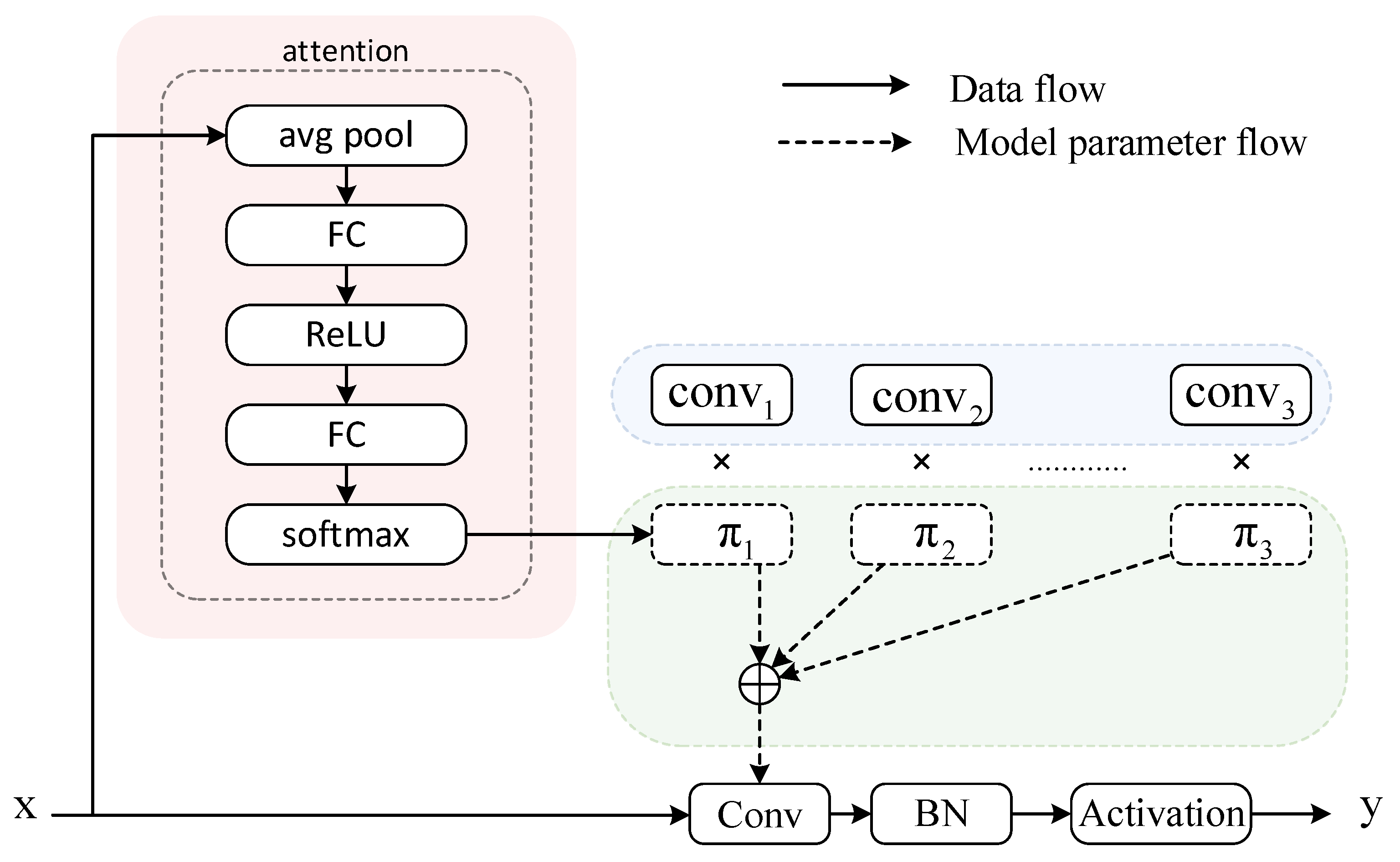
3.1.1. The Dynamic Convolution Module

Dynamic convolution represents an advanced convolutional neural network technique that enhances the models perception of input data by introducing variability and adaptability [26]. In comparison to the conventional static convolution, the principal benefit of dynamic convolution is its capacity to adapt the convolution kernel in accordance with the characteristics of the input features, thus facilitating the more effective capture and characterization of intricate structures and dynamic alterations within the data. It multiplies the number of parameters with almost no additional FLOPs added. The structure of Dynamic convolution is shown in Figure 2.

A dynamic convolution with M dynamic experts can be written as follows:

$$Y=X\ast W^{\prime },W^{\prime }={\displaystyle \sum _{i=1}^M{{\displaystyle \alpha }}_i}{{\displaystyle W}}_i$$

(2)

where $X\in {{\displaystyle R}}^{C_{in}\times H\times W}$ is the input feature, $Y\in {{\displaystyle R}}^{C_{out}\times H^{\prime }\times W^{\prime }}$ is the output feature, ${{\displaystyle W}}_i\in {{\displaystyle R}}^{C_{out}\times C_{in}\times H\times W}$ is the i-th convolution weight tensor, and ${{\displaystyle \alpha }}_i$ is the corresponding dynamic coefficient. ${{\displaystyle \alpha }}_i$ are dynamically generated based on different input samples. A typical way is to generate them based on the input using the MLP module, where $\alpha \in {{\displaystyle R}}^M$, as follows:

$$\alpha =soft\max (MLP(Pool(X)))$$

(3)

The coefficient generation in Equation (3) brings only negligible FLOPs compared to the original convolutional layer. In this way, multi-parameter networks implemented using dynamic convolution can dramatically increase more parameters while minimizing the increase in FLOPs.

For a standard convolutional layer, the number of parameters is $C_{out}\times C_{in}\times K\times K$ and the number of FLOPs is $H^{\prime }\times W^{\prime }\times C_{out}\times C_{in}\times K\times K$. Dynamic convolution includes a coefficient generation module, a dynamic weight fusion, and a convolution process. A coefficient generation module with $C_{in}$ hidden dimensions requires $C_{in}^2+C_{in}M$ parameters and $C_{in}^2+C_{in}M$ FLOPs. Dynamic weight fusion is parameter-free with FLOPs $M\times C_{out}\times C_{in}\times K\times K$. Therefore, the total number of parameters for dynamic convolution is $C_{in}^2+C_{in}M+M\times C_{out}\times C_{in}\times K\times K$, and the number of FLOPs is $C_{in}^2+C_{in}M+M\times C_{out}\times$$C_{in}\times K\times K+H^{\prime }\times W^{\prime }\times C_{out}\times C_{in}\times K\times K$.

The ratio of the parameters of dynamic convolution to standard convolution is

$$\begin{array}{cc}{R}_{param}\hfill & ={\displaystyle \frac{C_{in}^2+C_{in}M+M{C}_{out}{C}_{in}{K}^2}{C_{out}{C}_{in}KK}}\hfill \\ & ={\displaystyle \frac{C_{in}}{C_{out}{K}^2}}+{\displaystyle \frac{M}{C_{out}{K}^2}}+M\hfill \\ & \approx {\displaystyle \frac{1}{K^2}}+M\hfill \end{array}$$

(4)

where $M\ll C_{out}{K}^2,C_{in}\approx C_{out}$.

The ratio of FLOPs of dynamic convolution to standard convolution is

$$\begin{array}{cc}{R}_{flops}\hfill & ={\displaystyle \frac{C_{in}^2+C_{in}M+M{C}_{out}{C}_{in}{K}^2+H^{\prime }{W}^{\prime }{C}_{out}{C}_{in}{K}^2}{H^{\prime }{W}^{\prime }{C}_{out}{C}_{in}{K}^2}}\hfill \\ & ={\displaystyle \frac{C_{in}}{H^{\prime }{W}^{\prime }{C}_{out}{C}_{in}{K}^2}}+{\displaystyle \frac{M}{H^{\prime }{W}^{\prime }{C}_{out}{C}_{in}{K}^2}}+{\displaystyle \frac{M}{H^{\prime }{W}^{\prime }}}+1\hfill \\ & \approx 1\hfill \end{array}$$

(5)

where $1<M\ll H^{\prime }{W}^{\prime },C_{in}\approx C_{out}$.

It can be seen that the ratio of parameters of dynamic convolution and ordinary convolution is ${\displaystyle \frac{1}{K^2}}+M$, and the FLOPs of dynamic convolution and ordinary convolution are basically the same. This shows that the parameter amount of each dynamic convolution is about ${\displaystyle \frac{1}{K^2}}+M$ times that of conventional convolution, and the increase in calculation amount can be negligible.

3.1.2. The Online Re-Parameterization Module

Re-parameterization aims to enhance the performance of deep models without incurring additional inference–time costs. As illustrated in Figure 3a structure without re-parameterization lacks sufficient capacity to learn comprehensive information during the training phase. In contrast, Figure 3b depicts the standard structural re-parameterization approach, where multi-branch topologies are designed during training to replace the vanilla linear layers (e.g., conv or full connected layer) and improve model expressiveness. Afterward, during inference, the training-time complex models are transferred to simple ones for faster inference. While benefiting from complex training-time topologies, current re-parameterization methods are trained with non-negligible extra computational cost. When the block becomes more complicated for stronger representation, the GPU memory utilization and time for training will grow larger and longer, finally toward unacceptable. We propose a general online convolutional re-parameterization strategy, which makes the training-time structural re-parameterization possible.

Online re-parameterization (OREPA) [27] reduces the training overhead through two steps: block linearization and block squeezing. The compression of multiple branches in a linear manner, which results in a simplified model structure during training, has the potential to reduce the computational and storage overheads associated with intermediate layers. Furthermore, this approach can lead to a notable reduction in training consumption without any adverse impact on inference performance. Additionally, it enables the investigation of more intricate re-parameterization outcomes.

In the context of model architecture, the inclusion of Batch Normalization (BN) layers subsequent to each convolutional layer, as illustrated in Figure 3b, introduces significant computational and memory demands. The BN layer’s process of normalizing the feature map by its standard deviation is inherently nonlinear and must be performed independently for each branch, resulting in substantial computational load (high FLOPS) and memory consumption due to the buffering of feature maps. This leads to a considerable overhead during the training phase. Nevertheless, the scaling factor within the BN layer is crucial for directing the optimization of different branches; thus, indiscriminately eliminating the BN layer could result in a marked decrease in accuracy.

To address this issue, a linear Scaling layer is proposed as an alternative to the BN layer. This approach maintains the diversification of optimization directions across branches without incurring the same level of computational and memory costs associated with BN. Several alternatives to Batch Normalization have been proposed, such as Layer Normalization, Group Normalization, and Instance Normalization, each with its own limitations. Layer Normalization involves higher computational overhead due to the normalization of all features within a single sample. Group Normalization divides the channel dimension into multiple groups and normalizes features within each group, introducing additional hyperparameter tuning to determine the optimal group size. Instance Normalization normalizes each sample’s individual channels by computing the mean and variance for each channel independently. However, this method disregards information across batches and channels, making it unsuitable for tasks like defect detection, where preserving the global feature distribution is critical. The Scaling layer simplifies the normalization process, reducing the complexity and resource requirements while preserving the model’s accuracy. The linear Scaling layer can not only diversify the optimization directions of different branches like the BN layer but also combine calculations during training. The linearization block structure is shown in Figure 4. All nonlinear BN layers are deleted and Scaling is added to maintain the diversity of optimization.

In multi-branch architectures, each branch may learn different feature patterns, resulting in significant differences in output feature distributions. If these distribution discrepancies are directly passed to the next layer or involved in gradient computation, they may lead to gradient instability and affect model convergence. A Batch Normalization (BN) layer normalizes activation values, preventing them from becoming excessively large (exploding) or excessively small (vanishing), thereby ensuring that gradient magnitudes remain within a reasonable range during backpropagation. Therefore, to stabilize the training process, a BN layer is added after all branches.

Figure 5 illustrates the block structure diagram of the squeezing phase, and its main purpose is to reduce training costs while maintaining high performance. Define a two-dimensional convolution of size $K_H\times K_W$, and its convolution process is as follows:

$$Y=W\ast X$$

(6)

If a pile of convolutional layers is considered, as illustrated in Equation (7),

$$Y=W_N(W_{N-1}\dots (W_2(W_1\ast X)))$$

(7)

where $X\in R^{C_{\mathrm{i}}\times H\times W}$ and $Y\in R^{C_O\times H^{\prime }\times W^{\prime }}$ represents the input and output tensors, respectively, $W_j\in R^{C_{\mathrm{j}}\times C_{\mathrm{j}-1}\times K_{H_j}\times K_{W_j}}$ represents the weight of the layer $j$, and $C_i$ and $C_o$ represents the input and output channels, respectively.

Combined with the law, the convolution kernel can be compressed by the following equation to simplify the sequential structure, as in Equation (8),

$$Y=W_N(W_{N-1}\dots (W_2(W_1\ast X)))=W_e\ast X$$

(8)

where $W_e$ represents the end-to-end mapping matrix.

According to the linearity of the convolution, simplifying the parallel structure can merge multiple branches into one,

$$Y={\displaystyle \sum _{m=0}^{M-1}(W_m\ast X)}=({\displaystyle \sum _{m=0}^{M-1}{W}_m})\ast X$$

(9)

where $W_m$ is the weight of the m-th branch and ${\displaystyle \sum _{m=0}^{M-1}{W}_m}$ is the unified weight.

Block linearization and squeezing involve the precise merging and simplification of multiple branches, requiring meticulous adjustments and optimizations to the network architecture. Achieving weight sharing and structural compression across different branches while maintaining the model’s learning capability can significantly increase implementation complexity. In the original YOLOv8 model, the Bottleneck module features a single-branch sequential structure. To ensure manageable complexity, we retain the original single-branch structure and apply online re-parameterization to it.

First, drawing on the design principle of linear stage block, all nonlinear batch normalization (BN) layers within the Bottleneck module are removed and replaced with linear scaling layers to maintain the diversity of optimization directions. To ensure the stability of the training process, a BN layer is added after the branching. Then, using the design idea of compression phase block, the linear scaling layer is further compressed into the OREPA module, which not only maintains the high performance of the model, but also reduces the training cost. The enhanced version of the Bottleneck module has been rebranded as the Op-Bottleneck, and the C2f module has been upgraded to the C2f-OREPA module. This advancement simplifies the intricate structure to a streamlined single convolutional layer, which is a key factor in substantially lowering the training expenses. Despite this simplification, the C2f-OREPA module continues to deliver high performance, ensuring that the model remains efficient and effective without the excessive computational burden associated with more complex architectures. The model processing procedure and final structure are shown in Figure 6.

3.2. Multiscale Input-Aware MSA-SPPF

In defect detection tasks, feature extraction and fusion are the key links to ensure high detection accuracy. Although the existing defect detection models perform well in some specific scenarios, the size of defects in the image can vary greatly. Traditional single-scale feature extraction methods often fail to effectively capture defects of various sizes, resulting in reduced detection accuracy. Therefore, Multi-Scale Aware SPPF (MSA-SPPF) is proposed, which enhances the diversity of feature extraction and the flexibility of attention mechanism by integrating adaptive pooling layer and deformable large kernel attention mechanism, thus improving the robustness and accuracy of defect detection.

The SPPF module, while adept at capturing edge details, tends to overlook broader contextual information. To address this, the module has been enhanced by incorporating both global average pooling and global maximum pooling layers. These additions integrate comprehensive background and edge data, enabling the network to achieve more informed decisions. This enhancement facilitates the acquisition of a holistic view of the input and mitigates the effects of varying scales within the data.

Figure 7b illustrates the structure of the Deform-DW Con2D module, which leverages Deformable Convolutions to adjust sampling grid positions dynamically. An additional convolutional layer learns the offset field from the feature maps, generating adaptive sampling point shifts based on input features. This mechanism allows the convolutional kernel to reshape according to spatial feature variations, enabling more precise feature extraction [28].

The Deformable Large Kernel Attention (D-LKA) module processes the input feature map F by first applying a deformable depthwise convolution (ConvDDW), followed by a deformable depthwise dilated convolution (ConvDDW-D). The resulting feature map is then passed through a 1 × 1 convolutional layer (Conv2D). Finally, this output is added element-wise to the original input feature map F, effectively integrating the attention mechanism to enhance feature representations.

$$A\mathrm{ttention}=Con{v}_{1\times 1}(C{\mathrm{onv}}_{DDW-D}(Con{v}_{DDW}(F^{\prime })))$$

(10)

$$Output=A\mathrm{ttention}+\mathrm{F}$$

(11)

The structure of MSA-SPPF is shown in Figure 8.the input feature map x first passes through the basic convolution layer cv1 to adjust the number of channels, and then passes through the maximum pooling layer m twice. The kernel size is k, the step size is 1, and the filling is k/2. At the same time, x is also reduced to 1 × 1 through the adaptive maximum pooling layer AM and the adaptive average pooling layer AA. These feature maps are spliced in the channel dimension, and the convolution kernel is then dynamically adjusted through the DLKA module to capture local features. Finally, the final feature map is output through the base convolutional layer cv2. The MSA-SPPF module enables the network to enhance the perception of multi-scale features while maintaining spatial information, adapt to local shape changes through Deformable Convolution, and improve feature extraction accuracy and model performance.

3.3. Re-Parameterized Detection Head

The detection head of YOLOv8n adopts a single-scale prediction structure, which has few prediction head parameters and limited expression ability, so it is difficult to mine the spatial structure information in the features. At the same time, as a key part of the model, the detection head occupies almost 1/5 of the calculation amount of the model, which not only has a negative impact on the real-time reasoning of the model, but also affects its deployment on resource-constrained devices.

Therefore, this paper introduces the re-parameterized convolution (RepConv) to increase the ability of feature learning without increasing GFLOPs (only slightly improved), thus not affecting the reasoning speed and performance of the model. Its core idea is to use reparameterization technology to convert the parameters of the detector head into a better distribution, so as to improve the learning ability of the model for difficult samples.

RepConv is a simple but powerful convolutional neural network architecture. Its body is similar to VGG at inference time, except that it is composed of 3 × 3 convolution and ReLU stacked, while the model has a multi-branch topology at training time [29]. Decoupling the architecture during training and inference through structural reparameterization techniques. The information in the multi-branch structure is captured during training, the weights and biases of each branch are learned, and the equivalent convolution kernels and biases are computed during inference, compressing this information into a linear form to approximate the original multi-branch structure by a single convolution operation. This design facilitates exploring richer feature representations during training while maintaining an efficient reasoning process after training is completed. Figure 9 shows the structure of training and inference and Figure 10 shows the structure of RepHead.

4. Results and Analysis

4.1. Experimental Environment

In the experimental setup, the hardware specifications included an NVIDIA GeForce RTX 4060 Laptop GPU and 8188MiB of RAM. The software environment was Windows 11, with Python 3.9.19 as the programming language. The deep learning framework utilized was torch-2.0.0+cu118, which is equipped with an accelerated computing architecture. To prevent memory overflow, the batch size was configured to 8. The training regimen involved a learning rate of 0.01, and the momentum for stochastic gradient descent (SGD) was set at 0.937. Mosaic data augmentation was implemented to enhance the training process. The input images were resized to a resolution of 640 × 640 pixels. Training was conducted over 150 epochs with a consistent batch size of 8. For the non-maximum suppression (NMS) operation, an IoU threshold of 0.5 was applied to refine the detection results.

4.2. Dataset

The NEU-DET dataset, released by Northeastern University, is a collection of images designed for the development and evaluation of surface defect detection algorithms for hot-rolled steel strips. This dataset comprises 1800 grayscale images, each measuring 200 × 200 pixels, and includes six distinct types of defects: Rolled-in Scale, Patches, Crazing, Pitted Surface, Inclusion, and Scratches, with 300 instances of each defect type. The dataset is divided into a training set and a test set in a ratio of 8:2, resulting in 1440 images for training and 360 for testing. Annotations were created using the Labeling tool and converted from xml to txt format to facilitate YOLO training.

The dataset is noted for its intra-class variability and inter-class similarities, which pose challenges for algorithm development. Furthermore, due to variations in lighting conditions and material properties, the gray-scale values within images of the same defect type can differ significantly. This variability adds complexity to the task of developing robust defect detection algorithms, as it requires the algorithms to be adaptable to changes in image intensity and texture across different samples.

4.3. Evaluation Metrics

Precision is defined as the proportion of true positive instances among all instances that were identified as positive. The mathematical representation of this concept is given by

$$precision={\displaystyle \frac{TP}{TP+FP}}$$

(12)

here, $TP$ denotes the count of instances that are both actually and predicted to be positive, while $FP$ signifies the count of instances that are incorrectly predicted as positive.

Recall, on the other hand, is the proportion of true positive instances among all actual positive instances. Its formula is expressed as

$$recall={\displaystyle \frac{TP}{TP+FN}}$$

(13)

In this context, $FN$ represents the instances that are actually positive but were not identified as such.

Mean Average Precision (mAP) is the mean of the Average Precision (AP) values across all defect categories. AP is calculated as the area under the precision-recall curve. The formulas for AP and mAP are as follows:

$$AP={\displaystyle {\int }_0^{1}P(r)}dr$$

(14)

$$mAP={\displaystyle \frac{1}{N}}{\displaystyle {\sum }_{i=1}^{N}A{P}_i}$$

(15)

A higher mAP value indicates a better overall detection performance of the model across all defect categories.

Model parameters, denoted as Params, are the aggregate number of parameters within all convolutional layers and their corresponding kernels. Floating Point Operations (FLOPs) are a metric that quantifies the computational intensity of machine learning models. The calculation of FLOPs is depicted by the following formula:

$$FLOPs=(2\times C_{in}\times K^2-1)\times W_{out}\times H_{out}\times C_{out}$$

(16)

where $C_{in}$ represents the number of input channels and $K$ is the kernel size. $W_{out}$ and $H_{out}$ represent the width and height of the output feature map, respectively. $C_{out}$ indicates the number of output channels. This paper employs FLOPs as a metric to assess and compare the computational complexity of different models.

4.4. Ablation Experiment

A series of ablation experiments were performed on the NEU-DET dataset to evaluate the performance of each module proposed herein. The experimental results show the parameter quantity, computational complexity, and performance of the model under mAP @ 0.5 and mAP @ 0.5:0.95 indicators at different stages. Take YOLOv8n as the benchmark (model A), add model B of MSA-SPPF, add model C of Dconv, add C2f-OREPA to form model D, and finally introduce model E of RepHead. Ablation experiments showed the effect of each module on performance, as shown in

Table 1. Comparison of ablation experiments.

Models	Models Structure	Precision (%)	Recall (%)	Params/M	FLOPs/G	mAP @ 0.5 (%)	mAP @ 0.5: 0.95 (%)
A	YOLOv8n (baseline)	67	70.8	3.012	8.2	73.4	43.4
B	A + MSA SPPF	72.9	65.9	8.368246	12.3	74	43.6
C	B + Dconv	68.5	70.4	10.099998	11.1	75.2	43.7
D	C + C2f-OREPA	66.8	71.4	10.661790	10.6	75.3	44.4
E	D + RepHead	68.9	71.4	11.696094	10.7	75.7	44.5

.

The experimental results show that Model A achieves 0.6% and 0.2% growth on mAP @ 0.5 and mAP @ 0.5:0.95 indicators after integrating the MSA-SPPF module. This improvement is attributed to the fact that the MSA-SPPF module adopts global average pooling layer and global maximum pooling layer. By adding global background information and edge information, it can obtain global perspective information and mitigate the influence of different scales, so as to avoid information loss caused by traditional pooling operations. By introducing innovative deformable large kernel attention, the models attention in different feature receptive fields is enhanced, the models understanding of image targets is enhanced, and more accurate detection results are provided. The attention mechanism enables the model to focus on key feature channels, further improving detection performance.

Furthermore, the mAP @ 0.5 and mAP @ 0.5:0.95 indexes of Model B increased by 1.3% and 0.8%, respectively, after introducing multi-parameter network. Specifically, they increased by 1.2% and 0.1%, respectively, after adding Dconv, and increased by 0.1% and 0.7% after adding C2f-OREPA. It shows that the multi-parameter network idea can significantly improve the model performance. Furthermore, although the amount of parameters of the model has increased by about 2 M, the amount of computation has decreased by 1.7 G. These results show that the multi-parameter network not only improves the detection accuracy, but also shows advantages in the amount of parameters and calculations.

In Model E, after integrating the RepHead module, mAP @ 0.5 improves by 0.4%, while mAP @ 0.5:0.95 improves by 0.1%. This is because the RepHead module adopts the idea of using multi-branch auxiliary training during training and uses a double-branch structure to capture target information at different scales, which enhances the information transmission ability, alleviates the problem of gradient vanishing, and makes the model use of feature information more effectively. By strengthening information transmission, the RepHead module improves the expression ability and detection performance of the model.

Neural networks are perceived as “black box” methods, as the knowledge learned by the model is difficult to extract and present in a way that humans can understand. To “open the black box” and gain insight into how the network works, research on the interpretability of neural networks has emerged. CAM [30], Grad-CAM [31], and Grad-CAM++ [32] are widely recognized and applied techniques in deep learning for visualizing and understanding the decisions made by CNNs. CAM can only be used with the last feature map and relies on a global average pooling (GAP) operation, and it can only generate heatmaps for the final layer’s feature map, which makes it impractical for many real-world applications. Grad-CAM is a strict generalization of CAM, and unlike CAM, it is applicable to any CNN architecture without relying on GAP and it can generate heatmaps for any intermediate layer’s feature map. Grad-CAM++ is an optimized version of Grad-CAM; it provides better visual explanations of CNN model predictions, in terms of better localization of objects as well as explaining occurrences of multiple objects of a class in a single image.

Since industrial parts often have multiple defects of the same type on their surface, we use Grad-CAM++ to visualize the results of the MRP-YOLO model, providing an intuitive demonstration of the effects of models B, D, and E. Four samples were randomly selected. The output of the 21st layer of the network is visualized, and the score + box is back-propagated for gradient summation. The confidence level is 0.7, and the top 2% of data are sorted according to it to calculate the heat map. The experimental results are shown in Figure 11.

The results show that the MSA-SPPF module enhances Model B’s ability to capture contextual information and improves target detection performance in complex scenarios. The Dconv and C2f-OREPA modules give Model D more accurate target positioning capabilities, reducing missed and false detections. The final optimized model E has achieved significant improvement in feature extraction, the network weight distribution is more concentrated, and the suppression effect on non-defective areas is more obvious.

The existing ablation experiment (Table 1) has shown that introducing the RepHead module improves mAP@0.5 by 0.4% and mAP@0.5:0.95 by 0.1%. Although the improvement may appear marginal, the RepHead module is essential. We further compared the mean average precision (mAP) across different defect types to demonstrate the significant accuracy improvement achieved by RepHead for specific defects, as shown in

Table 2. Average accuracy results for six defects for Model D and Model E.

Model	Crazing	Patches	Inclusion	Pitted Surface	Rolled-in Scale	Scratches
D	35.2	80.8	84.2	80.8	60	91.7
E	41	93.9	85.1	79.4	61.1	93.1

. The table data reveal that the mean accuracy of all defect types improved, except for the Pitted Surface, while Patches experienced a remarkable increase of 12.9%.

4.5. Comparative Experiment

To assess the efficacy of MRP-YOLO, a comparative study, as detailed in

Table 3. Performance comparison of different algorithms.

Models	Precision (%)	Recall (%)	mAP (%)	mAP @ 0.5: 0.95 (%)	Params/M	FLOPs/G
YOLO v5n	65.2	70.1	73.3	41.6	2.504114	7.1
YOLO v5s	71.4	66.7	73.9	43.3	9.113858	23.8
YOLO v6s	65.3	69.3	73.7	40.2	16.298594	44
YOLO v6n	66.9	69.3	73.4	42	4.234338	11.8
YOLOv7-tiny	57.3	68.6	67.3	40.6	6.028	13.2
YOLO v8s	72	70	75	44	11.127906	28.4
YOLO v8n	67	70.8	73.4	43.4	3.012	8.2
ours	68.9	71.4	75.7	44.5	11.696094	10.7

, was conducted. The findings reveal that MRP-YOLO achieves the pinnacle of performance, with its Recall, mAP @ 0.5, and mAP @ 0.5:0.95 metrics peaking at 71.4%, 75.7%, and 44.5%, respectively, each representing the best outcomes. Although MRP-YOLO’s model size is marginally larger than YOLOv8n, necessitating additional computational resources, it maintains superior performance while only increasing FLOPs by approximately 2 million compared to YOLOv8n. Moreover, it boasts a reduction of around 18 million FLOPs compared to the less optimal YOLOv8s, underscoring MRP-YOLO’s efficiency. YOLOv6n strikes a balance, offering a moderate level of performance alongside manageable model complexity. On the other hand, YOLOv7-tiny falls short in terms of performance for a lightweight model, while YOLOv5s and YOLOv8s, despite their higher performance, are encumbered by larger model sizes and more complex computations. In conclusion, the enhancements made to the YOLOv8 network architecture through the MRP-YOLO algorithm have proven successful in streamlining the model and enhancing its performance.

Furthermore, YOLOv8n is selected as the baseline, and the experimental results of YOLOv8s, YOLOv6n, and YOLOv6s with better comprehensive performance in Table 3 are visualized together with the proposed MRP-YOLO, so as to more intuitively observe the changes in each index in the experimental process, as shown in Figure 12 and Figure 13.

Figure 12 shows the mAP curves for MRP-YOLO, baseline (YOLO v8n), YOLO v8s, YOLO v6n, and YOLOv6s during detection. The accuracy curve of MRP-YOLO rises the fastest during the early training stages. This is attributed to the MSA-SPPF module, which enhances the model’s multi-scale feature extraction capability through global average pooling and large-kernel attention mechanisms, enabling the model to quickly capture key features early in training and improve detection accuracy. In the mid-to-late training stages, MRP-YOLO’s accuracy curve stabilizes and reaches a peak accuracy of 75.7%. This is due to the RepHead detection head adopting a multi-branch structure during training, optimizing the feature representation of difficult samples, significantly reducing accuracy curve fluctuations, and improving the model’s overall performance. In comparison, the accuracy curves of the baseline YOLOv8n and YOLOv8s show slightly slower growth and lower final convergence points than MRP-YOLO, though both outperform YOLOv6n and YOLOv6s.

YOLOv6s and YOLOv6n exhibit the slowest convergence and the highest final loss values across all three loss functions: Training Box Loss, Training Classification Loss, and Training DFL Loss, indicating the poorest performance. In Figure 13a, the loss curves of YOLOv8s and YOLOv8n almost overlap, showing minimal difference, with both maintaining consistently higher loss values than MRP-YOLO. MRP-YOLO demonstrates the fastest decline in box position loss during the early training stages and ultimately stabilizes at a significantly lower value than the other models. Figure 13b shows that in the early stages, the losses of YOLOv8s and YOLOv8n are close to MRP-YOLO; however, after Epoch 80, MRP-YOLO’s loss decreases more substantially, converging to the lowest value. Figure 13c indicates that YOLOv8s experiences the fastest loss reduction and achieves the lowest final loss value, outperforming the other models.

Table 4. Average accuracy results for six types of defects.

Model	Crazing	Patches	Inclusion	Pitted Surface	Rolled-in Scale	Scratches
YOLOv5 n	35.4	93.1	82.8	78	59.1	91.5
YOLOv5s	38.3	93.1	82.2	82.1	56.8	90.9
YOLOv6 s	41.4	93.8	84.9	80.5	57.2	84.2
YOLOv7-tiny	28.4	87.8	71.9	81.4	52.4	82
YOLOv8 s	40.6	92.3	83.6	77.8	60.4	95.4
YOLOv8n	36.6	93.1	82.5	81.5	57.7	89.1
ours	41	93.9	85.1	79.4	61.1	93.1

shows the average accuracy of several YOLO models for various defect types. The data show that MRP-YOLO consistently outperforms the other models in terms of mean accuracy (mAP) in most defect categories. Notably, MRP-YOLO shows a clear advantage in detecting ‘Patches’, ‘Inclusion’, and ‘Rolled-in scale’ defects, with mAP scores of 93.9%, 85.1% and 61.1%. While the performance of the other models varied by category, YOLOv6s, YOLOv8s and YOLOv8n also all performed relatively well in terms of mAP in each defect category. In contrast, the YOLOv5 series and YOLOv7-tiny have much lower mAP compared to the other models in most categories. Overall, MRP-YOLO shows high accuracy in all defect categories, which demonstrates its strong recognition capability and improves the overall performance in recognizing a wide range of defect types.

The MRP-YOLO algorithm and YOLOv8n algorithm are used to train and test the dataset, and the defect detection effect is shown in Figure 14. Among them, the position of the defect is marked by a rectangular frame, rectangular frames of different colors are used for different types of defects, and the probability of defect detection is generated above the rectangular detection frame. Compared with the YOLOv8n algorithm, MRP-YOLO can better detect the position and type of defects, which verifies its superiority in performance improvement.

5. Conclusions

In this paper, a steel defect detection method based on YOLO v8 is proposed, which provides an effective method to solve the problems that the contrast of surface defects of industrial parts is not obvious and most of them are small target features, which leads to difficult feature extraction, low real-time detection efficiency, and slow speed and realizes efficient and accurate detection of defects.

• A multi-scale input-aware MSA-SPPF module is proposed, which adaptively extracts global background information and edge information, obtains global perspective information, and reduces the influence of different scales. The attention mechanism makes the model pay attention to the target area and ignore the background part, which enhances the anti-interference ability of the algorithm. At the same time, using its deformable and large convolution kernel characteristics, the model can appropriately adapt to different data patterns and fully understand the context;
• Using a multi-parameter network design method, dynamic convolution Dynamic Conv and innovative C2f-OREPA are used to avoid low FLOPS pitfall, which can improve performance through more data training and effectively reduce the computing resources required by the model. Dynamic Conv can better capture and characterize complex structures and dynamic changes in data by using the characteristics of dynamically adjusting convolution kernels based on input features. C2f-OREPA uses online reparameterization to convert complex structural re-parameters into single convolutional layers, which reduces the time-consuming of extensive training while maintaining feature expression capabilities;
• RepHead detection head is proposed to replace the traditional YOLOv8 detection head, and a single convolution operation is used to approximate the original trained multi-branch structure. While exploring richer feature representations during training, an efficient inference process is maintained after the training is completed.

Compared with other typical algorithms, the results show that the mAP (average accuracy mean) of the MRP-YOLO algorithm reaches 75.6%, which is 2.2% higher than that of the YOLOv8n algorithm, which shows that MRP-YOLO is more accurate in identifying and locating defects. In addition, the FLOPs (number of floating-point operations) of the MRP-YOLO algorithm are only 2.3 G higher than that of YOLOv8n, which means that while improving accuracy, the increase in computational complexity of the algorithm is limited, which is particularly important for scenarios that require real-time detection in resource-constrained industrial environments. Future work will focus on further optimizing the network model to achieve higher defect detection accuracy and faster detection speed.