Agricultural UAV Path Planning Based on a Differentiated Creative Search Algorithm with Multi-Strategy Improvement

Abstract

A differentiated creative search algorithm with multi-strategy improvement (MSDCS) is proposed for the path planning problem for agricultural UAVs under different complicated situations. First, the good point set and oppositional learning strategies are used to effectively improve the quality of population diversity; the adaptive fitness–distance balance reset strategy is proposed to motivate the low performers to move closer to the region near the optimal solution and find the potential optimal solution; and the vertical and horizontal crossover strategy with random dimensions is proposed to improve the computational accuracy of the algorithm and the ability to jump out of the local optimum. Second, the MSDCS is compared to different algorithms using the IEEE_CEC2017 test set, which consists of 29 test functions. The results demonstrate that the MSDCS achieves the optimal value in 23 test functions, surpassing the comparison algorithms in terms of convergence accuracy, speed, and stability by at least one order of magnitude difference, and it is ranked No. 1 in terms of comprehensive performance. Finally, the enhanced algorithm was employed to address the issue of path planning for agricultural UAVs. The experimental results demonstrate that the MSDCS outperforms comparison algorithms in path planning across various contexts. Consequently, the MSDCS can generate optimal pathways that are both rational and safe for agricultural UAV operations.

1. Introduction

An unmanned aerial vehicle (UAV) is an unmanned aerial vehicle that is operated by a remote control or automatic control system. In recent years, UAVs have been increasingly employed in agriculture due to their great flexibility, mobility, low safety risk factor, and low cost, and agricultural UAVs are unmanned aerial vehicles specifically designed for use in agriculture, which can significantly boost agricultural output, decrease expenses, and provide environmental benefit. For instance, UAVs may precisely spray crops using path planning, ensuring uniform coverage [1]. UAVs can fly along prearranged routes and gather data on crop growth to assist farmers in making more informed management choices [2]. UAVs can use path planning to conduct regular inspections of fields, monitor soil moisture and crop water storage with on-board sensors, and direct the irrigation system for precision irrigation [3]. UAVs can make 3D maps of farms to help farmers understand the topography of their farmland and plan irrigation systems and agricultural planting [4]. UAVs can be used to assess crop damage and offer data support to agricultural insurers, helping farmers obtain compensation more quickly [5].

Path planning is a key function for UAV mission execution and is a major challenge for autonomous UAVs in engineering applications. The current UAV path planning algorithms fall into two broad categories: classical and meta-heuristic algorithms. Classical algorithms include the Rapid Random Number Method based on random sampling (RRT) [6], the A* algorithm [7], and so on; these algorithms are less efficient in searching and converge slowly in complex situations. Path planning problems are classic NP hard problems with intricate constraints that make it difficult for general solvers to discover accurate solutions. Meta-heuristic algorithms can effectively solve complex combinatorial optimization problems. Common meta-heuristic algorithms include genetic algorithms (GAs) [8], ant colony optimization algorithms (ACOs) [9], gray wolf optimization algorithms (GWOs) [10], Harris Hawk optimization algorithms (HHOs) [11], whale optimization algorithms (WOAs) [12], sine cosine algorithms (SCAs) [13], and slime mold optimization algorithms (SMAs) [14].

Meta-heuristic algorithms are widely used in the study of UAV path planning. For example, Chen et al. [15] proposed an enhanced version of the chimp optimization algorithm to address the UAV path planning problem in a 3D environment. Zhang et al. [16] proposed an improved adaptive gray wolf optimization algorithm to address the three-dimensional path planning problem of UAVs in the complicated environment of material conveying in earthquake disaster zones. Wang et al. [17] proposed an updated bionic tuna swarm optimization algorithm for planning UAV flight paths safely and efficiently in complicated obstacle situations. Li et al. [18] proposed an improved particle swarm optimization algorithm for balancing the development and exploration capabilities of UAVs. He and Wang [19] proposed an improved chaos sparrow search algorithm to address the issue of delayed convergence and falling into local optimums in path planning in three-dimensional complicated environments for UAVs. Yu et al. [20] used a hybrid gray wolf optimization and differential evolutionary algorithm to tackle the UAV path planning problem. These algorithms can swiftly identify effective pathways by employing various search techniques across several iterations.

However, one of the most important difficulties remains: how to keep the algorithm from falling into a local optimum [21]. To enhance the path smoothness of agricultural UAVs in complex environments and achieve a reasonable and safe flight path, this study recognizes the agricultural UAV path planning problem as a complex optimization problem that necessitates an effective solution. It then suggests a multi-strategy improvement-based differentiated creative search algorithm (MSDCS) for agricultural UAV path planning. The differentiated creative search algorithm (DCS) is a novel meta-heuristic optimization algorithm proposed by Duankhan et al. [22] in 2024. The DCS is a model for iterative optimization of team performance that uses differential knowledge acquisition and creative realism strategies to solve complex optimization problems. While it is effective at solving complex optimization problems, it suffers from a lack of search accuracy and does not adequately explore unknown regions in the search space. This may result in agricultural UAVs not being reasonably fast or smooth for path planning in complex environments. Therefore, in this paper, a set of good points is used to resolve the uneven distributional problem in the initial population of the original DCS, and the oppositional learning strategy is used to improve the quality of the population and strengthen the algorithm’s search ability. To bring low performers closer to the region near the optimal solution, an adaptive fitness–distance balance reset strategy is proposed, which helps the algorithm search meticulously near the optimal solution to find the potential optimal solution. To address the issue that the DCS algorithm aggregates population individuals to the optimal individuals in later iterations, which can easily lead to search stagnation and the population falling into the local optimum, a vertical and horizontal crossover strategy with random dimensions based on the stochastic dimension is proposed to improve the algorithm’s computational accuracy, as well as its ability to jump out of the local optimum. A comparison with different algorithms through 29 test functions from the CEC2017 test set shows that the MSDCS possesses better convergence, and the stronger comprehensive performance of the MSDCS is further verified using the Wilcoxon rank-sum test and Friedman test. Finally, different agricultural UAV environment models were established to carry out simulation experiments on the trajectories of agricultural UAVs, and the applicability of the MSDCS in the agricultural UAV path planning problem was verified [23]. The main contributions of the novel algorithm proposed in this study are as follows:

(1)

The performance of the algorithm is enhanced, and a new optimization method for path planning of agricultural UAVs is developed by utilizing a good point set and oppositional learning strategy, an adaptive fitness–distance balance reset strategy, and a vertical and horizontal crossover strategy with random dimensions based on the original DCS algorithm.

(2)

Comparing the proposed algorithm with nine other algorithms, simulation experiments based on the CEC2017 test set validated the effectiveness of the MSDCS and further validated its comprehensive performance using the Wilcoxon rank-sum test and Friedman test.

(3)

The MSDCS is applied to the agricultural UAV path planning problem to minimize the objective function of the problem, which has complicated constraints. The results show that the MSDCS can generate high-quality solutions for agricultural UAV path planning, even in complex environmental conditions. Thus, a reasonable and safe flight path was obtained.

The remainder of this paper is organized as follows. Section 2 introduces the basic differentiated creative search algorithm; Section 3 describes, in detail, the three improvement strategies of the MSDCS; Section 4 calculates the time complexity of the MSDCS; Section 5 describes the environment, parameters, and result analysis of the simulation experiments; Section 6 models and experiments the agricultural UAV path planning problem; Section 7 discusses the results of the MSDCS in agricultural UAV path planning; and Section 8 summarizes the research of this paper.

2. Differentiated Creative Search Algorithm

2.1. Population Initialization

The process of the DCS algorithm is as follows. A set of candidate solutions $X$ (team members) is randomly generated with upper and lower bounds. Equation (1) is shown as follows:

$$X=\left[\begin{array}{ccccc}{x}_{1,1}& \dots & x_{1,d}& x_{1,D-1}& x_{1,D}\\ x_{i,1}& \dots & x_{i,d}& x_{i,D-1}& x_{i,D}\\ \dots & \dots & \dots & \dots & \dots \\ x_{NP-1,1}& \dots & x_{NP-1,d}& x_{NP-1,D}& x_{NP-1,D}\\ x_{NP,1}& \dots & x_{NP,d}& x_{NP,D}& x_{NP,D}\end{array}\right]$$

(1)

where $X_i$ denotes the $i$th candidate solution, $X_{i,d}$ denotes the $d$th location of the candidate solution, $NP$ represents the number of candidate solutions, and $D$ represents the dimension of the optimization problem. Each element of $X$ is randomly generated by Equation (2) as follows:

$$X_{i,d}=l{b}_d+U_i\left(0,1\right)\ast \left(u{b}_d-l{b}_d\right)$$

(2)

$l{b}_d$ and $u{b}_d$ are the lower and upper bounds of the optimization problem, respectively, and $U$ represents a uniform distribution in the interval $\left(0,1\right)$. After initialization, each individual is evaluated to determine their fitness value. Then, the individuals in $X$ are ordered based on their fitness value, with a smaller fitness value indicating higher performance.

2.2. Differentiated Knowledge Acquisition

The stages of differentiated knowledge acquisition are rooted in the different potentials for knowledge acquisition and can be categorized into three types, depending on the individual’s ability and level of performance. The first type of individual is the high performer, and these members serve as team idea generators and have a mindset that generates a diverse range of ideas; the second type of individual is the average performer, who serve as concept refiners, examining and comparing several ideas to determine the optimal answer; and the third type of individual is the low performer, and these members contribute to the team’s diversity and exploration by offering new ideas and approaches to problem solving. The process of updating the position of each individual can be executed using the following Equations (3)–(6), in which the poorer performers need to assimilate new knowledge or experience more than the better performers:

$$X_{i,d}=\left\{\begin{array}{c}Xnex{t}_{i,d}, if{U}_{i,d}\left(0,1\right)\le {\delta }_i or d=j_{rand}\\ X_{i,d}, otherwise\end{array}\right.$$

(3)

$${\delta }_i\leftarrow {\displaystyle \frac{\left[U_i\left(0,1\right)\ast {\phi }_i\right]+\left(U_i\left(0,1\right)\le {\phi }_i\right)}{2}}$$

(4)

$${\phi }_i=0.25+0.55\ast {\left({\displaystyle \frac{R_i}{NP}}\right)}^{0.5}$$

(5)

$$j_{rand}=randint\left(1,D\right)$$

(6)

As stated in Equation (3), $U_{i,d}\left(0,1\right)$ denotes a random number that ranges between 0 and 1 and is generated independently for each dimension of each particle. If the condition is met, the position is updated by Equation (7), otherwise, the position remains unchanged. Where parameter ${\delta }_i$ is the quantitative knowledge acquisition rate of the $i$th individual at the $t$th iteration, and the uniformly distributed random numbers generated by the two $U$’s in Equation (4) are different, with the first half $\left[.\right]$ indicating rounding to the nearest whole number, while the second half compares the random number with ${\phi }_i$, and, if true, the value is 1; otherwise, the value is 0. ${\phi }_i$ represents the variable $\phi$’s value at the $t$th iteration of an individual, while $R_i$ represents the $i$th individual’s ranking at the start of the $t$th iteration. The $\phi$ coefficient measures the degree of imperfection in an individual’s knowledge. Higher values indicate larger gaps in knowledge and the need for additional learning and experience to compensate; smaller values indicate a more comprehensive and solid foundation in the relevant knowledge area. $j_{rand}$ is an integer chosen randomly from 1 to $D$ and is generated once per individual.

2.3. Creative Realism

The differential knowledge acquisition stated above divides teams into low, high, and average performers, and creative realism is based on the divergent thinking of high performers and the convergent thinking of average performers. Creative ideas and problem solving are both key characteristics of high performers. Not only do high performers serve as a knowledge basis, but each member of the team is required to constantly draw on fresh knowledge and broaden their divergent thinking. For the average performer, convergent thinking relies on the knowledge of the best individual, combined with random contributions from two different team members. The position update of an individual can be performed using the following Equations (7)–(9):

$$Xnex{t}_{i,d}=\left\{\begin{array}{c}{X}_{r1,d}+L{K}_{i,d}\left(\alpha ,\sigma \right), if i\le ngs\\ X_{best,d}+\gamma \ast \left(X_{r2,d}-X_{i,d}\right)+\omega \ast \left(X_{r1,d}-X_{i,d}\right), otherwise\end{array}\right.$$

(7)

$$ngs=\max \left(6,\left[NP\ast {\displaystyle \frac{g}{3}}\right]\right)$$

(8)

$$\gamma =0.1+0.518\ast \left(1-{\left({\displaystyle \frac{t}{\max \_it}}\right)}^{0.5}\right)$$

(9)

$X_{r1,d}$ represents the $d$th location of a randomly picked individual in $\left\{1,2,\dots ,NP\right\}$, and $L{K}_{i,d}\left(\alpha ,\sigma \right)$ is the Lévy flying random number generator with control parameters $\alpha$ and $\sigma$. $ngs$ stands for the number of high performers according to the population’s golden ratio, $g$, which will have a value of an integer larger than or equal to six. $X_{best,d}$ is the $d$th position of the best individual and $X_{r2,d}$ is the dth position of the individual randomly selected from $\left\{ngs+1,\dots ,NP\right\}$. $\omega$ denotes the learning intensity state of an individual, with a default value of 1. $\gamma$ is the coefficient of the individual at the $t$th iteration, $t$ is the current number of iterations, and $\max \_it$ is the maximum number of iterations. The $\gamma$ coefficient measures how much a team’s social dynamics influence an individual’s views. Higher values indicate a greater reliance on team members, while lower values indicate a greater degree of independence. The DCS algorithm replaces underperforming members with new ones to increase the diversity of ideas generated by the team. The formula for producing new members is given by Equation (10) as follows:

$$X_{i,d}=\begin{array}{c}l{b}_d+U_i\left(0,1\right)\ast \left(u{b}_d-l{b}_d\right), if i=NP \mathrm{and} U_i\left(0,1\right)<pc\end{array}$$

(10)

When $pc$ is 0.5, the method defaults to the last team member, and $U_i\left(0,1\right)<pc$ is an inefficiency and uses random initialization to reset the individual.

3. Improvement Strategies

3.1. Population Initialization Based on Good Point Set and Oppositional Learning Strategies

The distribution location of the initial population and the quality of the solution have a significant impact on the effectiveness of the metaheuristic algorithm [24]; if the initial population is too centralized or too dispersed, the algorithm may underutilize the search space, and if the quality of the solution in the population is low, the algorithm’s convergence accuracy will suffer. The original DCS algorithm’s random initialization is too unpredictable to ensure the algorithm’s population diversity and convergence accuracy. This study provides enhancements to its initialization procedure.

3.1.1. Good Point Set Strategy

In the optimization process of meta-heuristic algorithms, the diversity of the algorithm can be enhanced if the initialized population is made to be uniformly distributed over the spatial range of the objective function. The good point set [25] is an effective uniform point selection method with good distribution, so we use it to initialize the population in the MSDCS. Let $V_D$ be a $D$-dimensional Euclidean space unit cube, with $r\in V_D$. Then, the set of good points is formed in Equations (11) and (12) as follows:

$$P_{NP}\left(k\right)=\left\{\left(\left\{r_1\ast k\right\},\dots ,\left\{r_D\ast k\right\}\right),1\le k\le NP\right\}$$

(11)

$$r_i=2\cos {\displaystyle \frac{2\pi i}{p}},1\le i\le D$$

(12)

where $NP$ is the number of populations, $P_{NP}\left(k\right)$ is the set of good points, $r$ is the value of good points, and $p$ is the smallest prime number that satisfies ${\displaystyle \frac{p-3}{2}}\ge D$. Therefore, the initialization based on the set of good points is given by Equation (13) as follows:

$$X_{i,d}=l{b}_d+P_{NP}\left(k\right)\ast \left(u{b}_d-l{b}_d\right)$$

(13)

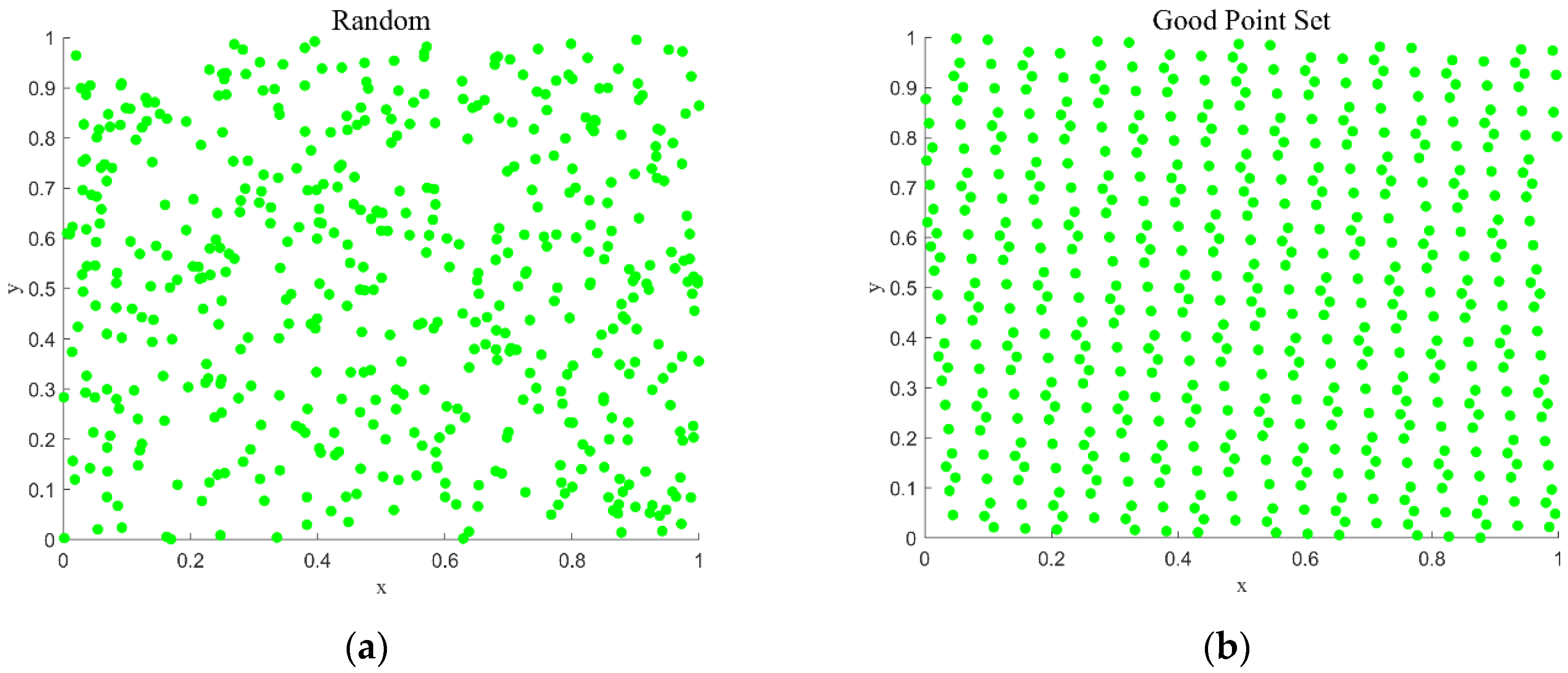
Theoretically, weighted sums formed with $n$ good points have smaller errors than those obtained with any other $n$ points, making them appropriate for approximate computations in higher dimensional spaces. Generate 500 points in a two-dimensional unit search space and compare the randomized points. The points from the good point set approach are shown in Figure 1.

Figure 1 shows that random points are not uniformly distributed, resulting in lower utilization of the algorithm’s search space, whereas points generated using the good point set method are more uniformly distributed in the search space, resulting in broader coverage of the population and improving the efficiency of the global search.

3.1.2. Oppositional Learning Strategy

Meta-heuristic algorithms typically save high-quality individuals from the previous generation population to the next generation population. The number of high-quality individuals in the initial population has a direct impact on the algorithm’s convergence rate; if there are fewer high-quality individuals in the initial population, the algorithm’s convergence speed and accuracy will suffer. Therefore, in this paper, we use an oppositional learning strategy to boost the number of quality individuals in the generated initial population. To be more precise, the algorithm simultaneously generates an individual who opposes the individual in the good point set. Finally, the individuals with the best fitness values are chosen as the beginning population, increasing the algorithm’s search efficiency. Their opposing positions ($X_{i,d}^{\prime }$) can be expressed by Equation (14) as follows:

$$X_{i,d}^{\prime }=l{b}_d+u{b}_d-X_{i,d}$$

(14)

The lower and upper bounds of the individual positions are $l{b}_d$ and $u{b}_d$, respectively. The implementation process of population initialization based on the good point set and oppositional learning strategy is as follows: generate an initial population based on the good point set, compute the oppositional population using Equation (14), rank the fitness values, and select the top $NP$ individuals with better fitness values as the new initial population. As shown in

Table 1. Test results of population initialization strategies. The DCS randomly generates initial points. DCS1 uses the good point set strategy only, while DCS2 uses both the good point set and oppositional learning strategies.

	DCS	DCS1	DCS2
F1	1.77 × 108	9.00 × 107	8.45 × 107
F4	9.39 × 102	8.94 × 102	8.62 × 102
F11	1.08 × 104	1.09 × 104	7.69 × 103
F29	8.34 × 103	8.12 × 103	7.31 × 103

, the best fitness values of four representative test functions were selected from the CEC2017 test set with 500 iterations of the algorithm and 30 independent runs. DCS1 uses the good point set strategy, and DCS2 uses the good point set and oppositional learning strategy. The results show that population initialization based on a good point set and an oppositional learning strategy can effectively improve the algorithm’s ability to find the optimal value.

3.2. Adaptive Fitness–Distance Balance Reset Strategy

The DCS algorithm categorizes team members into three types: low, high, and average performers. For the high performer, combining the existing knowledge and creative elements can provide better solutions to the innovation of the problem; for the average performer, refinement of the knowledge from the best team members promotes the diversity of solutions. However, for low performers, acquiring new knowledge only affects one dimension of an individual’s knowledge structure, as in Equation (10). This local variation contributes to diversity through random initialization and cannot ensure the quality of the solution. To encourage low performers to migrate closer to the optimal solution zone, this research presents an adaptive fitness–distance balance reset strategy. By dynamically adjusting the balance between randomized and targeted exploration, the strategy efficiently identifies the candidates with the highest potential from the population while maintaining diversity, enabling the algorithm to perform a detailed search on the area of good fitness to find a potentially better solution, as described in the following steps.

The first step is to compute the distance ($D_{Pi}$) between the present solution ($x_{Pi}$) and the best solution ($P_{best}$) using the Euclidean distance metric, which is mathematically modeled by Equation (15) as follows:

$$D_{Pi}=\sqrt{{\left(x_{P_i,1}-x_{P_{best},1}\right)}^2+\dots +{\left(x_{P_i,D}-x_{P_{best},D}\right)}^2}$$

(15)

The second step is to compute the candidate solution’s score ($S_{AFDB{P}_i}$), which is obtained by weighted summation of the normalized fitness value ($norm{F}_{P_i}$) and the normalized distance value ($norm{D}_{P_i}$) using Equations (16)–(18) as follows:

$$S_{FDB{P}_i}=w\ast norm{F}_{P_i}+\left(1-w\right)\ast norm{D}_{P_i}$$

(16)

$$norm{f}_{P_i}={\displaystyle \frac{f_{P_i}-\min \left(f\right)}{\max \left(f\right)-\min \left(f\right)}}$$

(17)

$$\mathrm{If} \mathrm{goal} \mathrm{is} \mathrm{minimization}\to norm{F}_{P_i}=1-\mathrm{norm}{f}_{P_i}$$

(18)

where $\max \left(f\right)$ and $\min \left(f\right)$ are the maximum and minimal fitness values, respectively, and the fitness value in the minimization problem is defined in Equation (18). The weighting coefficient $w$ is used to modify the effect of the fitness and distance values. In this study, $w$ is an adaptive operator with the following Equation (19):

$$w=\max \left(0.1, 0.9-{\displaystyle \frac{it}{\max \_it}}\right)$$

(19)

The value of $w$ decreases as the number of iterations increases, allowing for a fast exploration of the space based on the fitness value in the early stages, followed by a meticulous search as approaching the optimum in the later stages. Then, using Equation (20), the candidate with the highest score ($S_{maxFDB}$) is chosen to update the inefficient individual ($X_{i,d}$).

$$X_{i,d}=X_{i,d}+U_i\left(0, 1\right)\ast \left(S_{maxFDB}-X_{i,d}\right), if i>NP-10 \mathrm{and} U_i\left(0, 1\right)<pc$$

(20)

In the original DCS algorithm, the last individual is defined as inefficient and updated using random initialization, resulting in low-quality solutions. In this study, the algorithm designates the last ten individuals in the fitness ranking list as inefficient and then employs an adaptive fitness–distance balance reset technique to enhance their quality.

Table 2. The DCS and DCS3 test results. DCS3 shows the best fitness values obtained by the DCS algorithm plus the adaptive fitness–distance balance reset strategy.

	DCS	DCS3
F1	1.77 × 108	1.20 × 108
F4	9.39 × 102	9.07 × 102
F11	1.08 × 104	7.69 × 103
F29	8.34 × 103	6.93 × 103

shows the result of the best fitness value obtained by the DCS algorithm based on the adaptive fitness–distance balance reset strategy (DCS3) and the original algorithm (DCS) (the experimental setup is found in Section 3.1.2). It can be seen that the DCS algorithm based on the adaptive fitness–distance balance reset strategy has a better value of the best fitness in these test functions.

3.3. Vertical and Horizontal Crossover Strategy with Random Dimensions

In later iterations of the DCS, the individuals gradually converge to the optimal individual, and the fitness values of the individuals tend to stabilize. As a result, new and better solutions are difficult to emerge, which can easily lead to the search becoming stagnant and the population falling into the local optimum. To improve the convergence accuracy of the DCS and enhance the algorithm’s ability to jump out of the local optimum, this paper uses the vertical and horizontal crossover strategy based on random dimensions to improve the current individuals. Specifically, the horizontal crossover is used for searching to reduce the search blind spots and improve the algorithm’s global search ability; the vertical crossover is used to enhance population variety while decreasing the risk of the algorithm falling into the local optimum. The dimensions involved are selected by $c$, i.e., $c$ determines the number of dimensions involved in the vertical and horizontal crossings. Initially, a comprehensive random perturbation is performed, which is conducive to quickly jumping out of the local optimum, and with the increase in the number of iterations, the search is gradually centralized, which is conducive to fine optimization. The calculation process is given by Equation (21) as follows:

$$c=max\left[D-{\displaystyle \frac{it}{max\_it}}\ast \left(D-1\right),1\right]$$

(21)

The horizontal crossover refers to the exchange of individual information between two different members in a randomly chosen dimension so that different individuals can learn from each other. This operation can also be viewed as a mutating process of generating a new position based on two random individuals. The horizontal crossover of two unduplicated individuals of the team on $c$ randomly chosen dimensions $rd1$ generates offspring with Equations (22) and (23) as follows:

$${X^{\prime }}_{j,rd1}=r_1\ast X_{j,rd1}+\left(1-r_1\right)\ast X_{jj,rd1}+v_1\ast \left(X_{j,rd1}-X_{jj,rd1}\right)$$

(22)

$${X^{\prime }}_{jj,rd1}=r_2\ast X_{jj,rd1}+\left(1-r_2\right)\ast X_{j,rd1}+v_2\ast \left(X_{jj,rd1}-X_{j,rd1}\right)$$

(23)

In this equation, ${X^{\prime }}_{j,rd}$ and ${X^{\prime }}_{jj,rd}$ are the individuals generated by $X_j$ and $X_{jj}$ after the horizontal crossover; in this way, each mutation operation affects only the values on the selected dimension, while the other dimensions remain unchanged. $r_1$ and $r_2$ are random numbers of $\left[0,1\right]$ used for balancing the individual’s current position in each mutation operation, and $v_1$ and $v_2$ are random numbers of $\left[-1,1\right]$ used for regulating the distance between the individual’s current position and crossover point position in each mutation operation. The resulting children compete with the parent generation, and the best individuals are finally retained.

The vertical crossover of this strategy implies that the best individuals in the population exchange information across randomly selected dimensions, resulting in a new generation of the best individuals to compete with the parent generation, allowing different dimensions to learn from one another and avoiding premature convergence of one dimension. The individual formulae for the offspring obtained from the vertical crossover are given by Equation (24) as follows:

$$Xbes{t^{\prime }}_{rd2}=q\ast Xbes{t}_{rd2}+\left(1-q\right)\ast Xbes{t}_{rd3}$$

(24)

The offspring individual $Xbes{t^{\prime }}_{rd2}$ is created via the vertical crossover of the present optimal individual $Xbest$ on $c$ randomly chosen dimensions $rd2$ and $rd3$ ($rd2\ne rd3$). $q \in \left[0,1\right]$ is used to control the magnitude of the shift of the new position during the vertical crossover.

Table 3. The DCS and DCS4 test results. DCS4 depicts the results of the DCS with the random dimension-based vertical and horizontal crossover strategy.

	DCS	DCS4
F1	1.77 × 108	7.63 × 103
F4	9.39× 102	6.74 × 102
F11	1.08× 104	2.01 × 103
F29	8.34 × 103	6.05 × 103

depicts the results of the random dimension-based vertical and horizontal crossover strategy (DCS4) and the original algorithm (DCS) in the test function (the experimental setup is the same as above). The test results of DCS4 are significantly better than the DCS.

4. Time Complexity

The basic DCS algorithm has a total time complexity of $O\left(N\ast D\ast T\right)$, where $N$ is the population size, $D$ is the dimension, and $T$ is the maximum number of iterations. The time complexity of the MSDCS algorithm is evaluated as follows.

The process consists mostly of population initialization, fitness evaluation, and updating candidate solutions. The temporal complexity of population initialization is $O\left(N\ast D\right)$, and fitness evaluation is $O\left(N\right)$. The candidate solution is updated in four steps. First, when the team is inefficient, the time complexity is $O\left(T\ast pc\right)$, where $pc$ is a probability constant. Second, the time complexity of updating the candidate solution when the team is efficient is $O\left(T\ast ngs\ast D\ast \delta \right)$, where $ngs$ denotes the number of high-performance candidates and $\delta$ denotes the knowledge acquisition rate. Then, the time complexity of updating the candidate solution when the team is average is $O\left(T\ast \left(N-ngs-1\right)\ast D\ast \delta \right)$. Finally, the time complexity of updating the candidate solutions using the vertical and horizontal crossover strategy with random dimensions is $O\left(N\ast D\right)$. In summary, excluding the low-order terms, the time complexity of the MSDCS is $O\left(N\ast D\ast T\right)$, which is the same as the original algorithm.

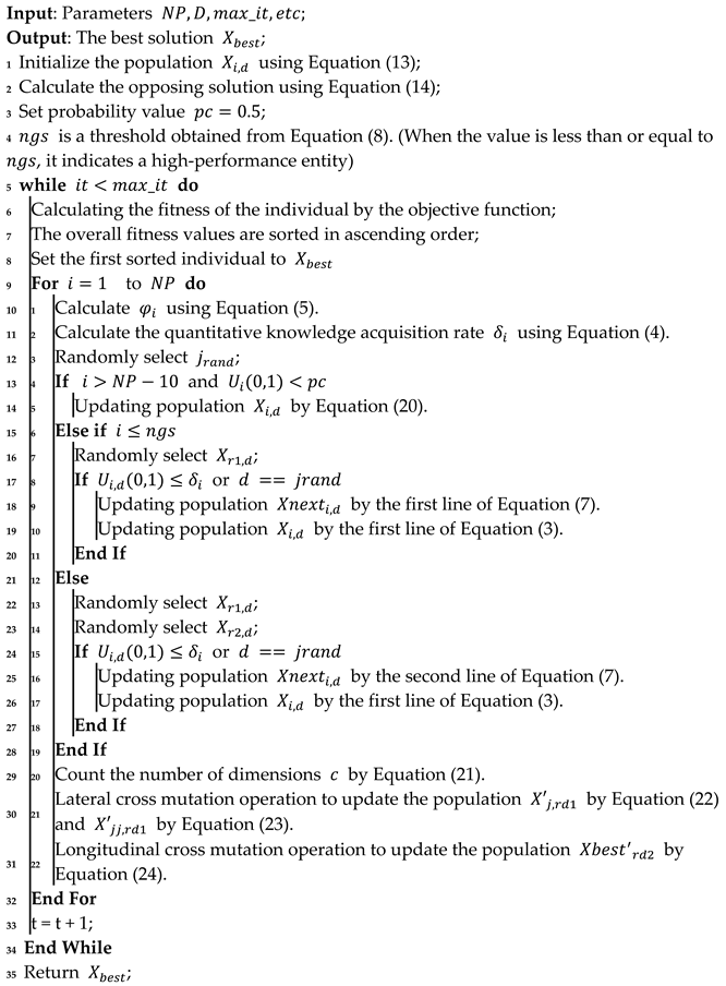
The pseudo-code for the improved Algorithm 1 is as follows.

Algorithm 1: MSDCS

5. Simulation Experiment and Result Analysis

5.1. Test Functions and Experimental Environments

To test the optimization ability of the proposed MSDCS algorithm, 29 test functions from the CEC2017 test set are chosen, and the specific function information is shown in

Table 4. Descriptions of CEC2017.

Class	ID	Functions	${\mathit{f}}_{\mathit{m}\mathit{i}\mathit{n}}$
Unimodal Functions	F1	Shifted and Rotated Bent Cigar Function	100
	F3	Shifted and Rotated Zakharov Function	300
Simple Multimodal Functions	F4	Shifted and Rotated Rosenbrock’s Function	400
	F5	Shifted and Rotated Rastrigin’s Function	500
	F6	Shifted and Rotated Expanded Scaffer’s F6 Function	600
	F7	Shifted and Rotated Lunacek Bi_Rastrigin Function	700
	F8	Shifted and Rotated Non-Continuous Rastrigin’s Function	800
	F9	Shifted and Rotated Levy Function	900
	F10	Shifted and Rotated Schwefel’s Function	1000
Hybrid Functions	F11	Hybrid Functions 1 (N = 3)	1100
	F12	Hybrid Functions 2 (N = 3)	1200
	F13	Hybrid Functions 3 (N = 3)	1300
	F14	Hybrid Functions 4 (N = 4)	1400
	F15	Hybrid Functions 5 (N = 4)	1500
	F16	Hybrid Functions 6 (N = 4)	1600
	F17	Hybrid Functions 6 (N = 5)	1700
	F18	Hybrid Functions 6 (N = 5)	1800
	F19	Hybrid Functions 6 (N = 5)	1900
	F20	Hybrid Functions 6 (N = 6)	2000
Composition Functions	F21	Composition Functions 1 (N = 3)	2100
	F22	Composition Functions 2 (N = 3)	2200
	F23	Composition Functions 3 (N = 4)	2300
	F24	Composition Functions 4 (N = 4)	2400
	F25	Composition Functions 5 (N = 5)	2500
	F26	Composition Functions 6 (N = 5)	2600
	F27	Composition Functions 7 (N = 6)	2700
	F28	Composition Functions 8 (N = 6)	2800
	F29	Composition Functions 9 (N = 3)	2900
	F30	Composition Functions 10 (N = 3)	3000

. The CEC2017 test set [26] is challenging and widely used in academic studies. All functions in the test set were rotated and shifted to increase the difficulty of optimization and avoid bias caused by the solution space’s symmetry. The functions can be divided into four categories: single peak, multi-peak, hybrid, and combined functions. The single-peak function has only one optimal solution, which is used to measure the algorithm’s convergence speed and local search ability, whereas the other three types of functions have multiple solutions, which are used to test the algorithm’s ability to escape from local optima and explore globally. F1 and F3 are single-peak functions with no local optimum and just a global optimum (F2 was officially deleted due to its instability); F4–F10 are multi-peak functions having local extreme points; F11–F20 are hybrid functions; and F21–F30 are combination functions. All experiments were performed in the same environment with a Win10 64-bit operating system, an AMD Ryzen 7 4800H processor with Radeon Graphics at 2.90 GHz, and 16 GB of RAM, and produced by Lenovo in Beijing, China.

5.2. Overview of Convergence Analysis and Comparative Algorithms

The comparison algorithms contain two classical algorithms, including the particle swarm optimization algorithm (PSO) [27] and the differential evolution algorithm (DE) [28]; two newly proposed algorithms, including the black-winged kite optimization algorithm (BKA) [29] and the snow ablation optimization algorithm (SAO) [30]; two recent improved algorithms, including the improved sand cat swarm optimization algorithm (MSCSO) [31] and the dispersed foraging slime mold algorithm (DFSMA) [32]; and two representative competition algorithms, including the linear population reduction SHADE algorithm (LSHADE) [33] and the improved multi-objective differential evolutionary algorithm (IMODE) [34]. Two typical intelligent optimization algorithms, the PSO and DE, are selected as the baseline algorithms for their stability and extensive application; the BKA and SAO are both new algorithms proposed recently, which are new breakthroughs in related research fields; the MSCSO and DFSMA add new strategies into their original algorithms and have better performance, similar to the present MSDCS; and the LSHADE and IMODE have proved their excellent performance in practical applications in open competitions. Since there is no improved algorithm based on the DCS yet, the comparison with these comprehensive algorithms can verify the proposed MSDCS algorithm’s superiority in optimization performance. As a result, with the additional DCS algorithm, there are nine algorithms to be compared with the MSDCS algorithm. In this research, the population size $N$ of all algorithms is set to 30, the maximum number of iterations $T$ is set to 500, the dimension $D$ is 100, and each method is run independently 30 times. Additional parameters are presented in

Table 5. Parameter settings for comparative algorithms.

Algorithm	Parameter Settings
PSO	$c_1=2$;$c_2=2$; $w=0.9$
DE	$Scaling factor=0.5$; $crossover probability=0.5$
BKA	$p=0.5$; $r\in \left(0, 1\right)$
SAO	$\theta \in \left[0, 1\right]$
MSCSO	$SM=2$; $\beta \in 0, 2\pi$; $Roulette Wheel selection\in \left[0, 360\right]$
DFSMA	Finding food operation probability $z$= 0.03,$DR\in \left[0, 0.4\right]$
LSHADE	$r^{N^{init}}=18D$, $p=0.11$,$H=6$
IMODE	$F=0.35$; $CR=0.2$
DCS	$pc=0.5$; $\omega =1$

. The performance of each algorithm’s optimization is measured using three performance indexes: optimal value, average value, and standard deviation, with the experimental results presented in

Table 6. Comparison of the test function results in CEC2017.

Function	Index	MSDCS	DCS	PSO	DE	BKA	SAO	MSCSO	DFSMA	LSHADE	IMODE
F1	Fbest	1.07 × 102	3.43 × 107	2.28 × 108	3.99 × 109	9.76 × 1010	4.48 × 109	4.00 × 1010	1.19 × 108	3.18 × 109	1.60 × 102
	mean	7.86 × 103	1.24 × 108	3.25 × 108	4.99 × 109	1.39 × 1011	7.94 × 109	6.96 × 1010	2.43 × 108	6.43 × 109	2.20 × 1010
	std	8.16 × 103	5.76 × 107	5.81 × 107	8.66 × 108	1.70 × 1010	2.15 × 109	1.24 × 1010	7.91 × 107	2.06 × 109	8.23 × 1010
F3	Fbest	3.13 × 104	1.94 × 105	3.89 × 105	6.51 × 105	2.33 × 105	5.55 × 105	2.38 × 105	2.62 × 105	2.31 × 105	3.00 × 102
	mean	6.15 × 104	2.79 × 105	5.09 × 105	8.31 × 105	2.66 × 105	9.13 × 105	2.83 × 105	4.14 × 105	4.14 × 105	3.01 × 102
	std	1.27 × 104	4.20 × 104	7.98 × 104	8.59 × 104	1.94 × 104	2.11 × 105	2.61 × 104	1.34 × 105	1.61 × 105	1.25
F4	Fbest	5.68 × 102	7.65 × 102	7.09 × 102	1.71 × 103	1.48 × 104	1.10 × 103	3.64 × 103	7.65 × 102	9.81 × 102	6.75 × 102
	mean	7.00 × 102	8.80 × 102	8.53 × 102	2.15 × 103	2.32 × 104	1.48 × 103	6.87 × 103	9.24 × 102	1.50 × 103	8.55 × 103
	std	5.79 × 10	5.55 × 10	6.24 × 10	2.85 × 102	6.71 × 103	2.01 × 102	2.39 × 103	8.39 × 10	3.33 × 102	2.92 × 104
F5	Fbest	1.01 × 103	1.23 × 103	1.26 × 103	1.59 × 103	1.36 × 103	1.45 × 103	1.34 × 103	1.11 × 103	9.53 × 102	1.58 × 103
	mean	1.09 × 103	1.34 × 103	1.39 × 103	1.66 × 103	1.52 × 103	1.64 × 103	1.49 × 103	1.29 × 103	1.20 × 103	1.80 × 103
	std	4.15 × 10	5.26 × 10	5.46 × 10	2.97 × 10	6.84 × 10	7.57 × 10	5.53 × 10	8.88 × 10	1.01 × 102	1.24 × 102
F6	Fbest	6.00 × 102	6.09 × 102	6.64 × 102	6.20 × 102	6.71 × 102	6.30 × 102	6.66 × 102	6.45 × 102	6.18 × 102	6.66 × 102
	mean	6.00 × 102	6.13 × 102	6.71 × 102	6.23 × 102	6.78 × 102	6.39 × 102	6.73 × 102	6.60 × 102	6.31 × 102	6.77 × 102
	std	1.57 × 10−1	2.30	4.31	2.09	3.39	5.71	3.54	6.37	5.75	1.16 × 10
F7	Fbest	1.40 × 103	1.68 × 103	2.03 × 103	2.03 × 103	3.21 × 103	2.11 × 103	2.88 × 103	1.90 × 103	2.04 × 103	3.59 × 103
	mean	1.54 × 103	1.84 × 103	2.33 × 103	2.14 × 103	3.38 × 103	2.36 × 103	3.26 × 103	2.26 × 103	2.42 × 103	5.37 × 103
	std	8.31 × 10	7.18 × 10	1.57 × 102	5.22 × 10	8.93 × 10	1.14 × 102	1.38 × 102	2.55 × 102	2.47 × 102	1.06 × 103
F8	Fbest	1.25 × 103	1.51 × 103	1.56 × 103	1.86 × 103	1.83 × 103	1.80 × 103	1.70 × 103	1.38 × 103	1.26 × 103	1.94 × 103
	mean	1.37 × 103	1.62 × 103	1.79 × 103	1.94 × 103	1.94 × 103	1.94 × 103	1.91 × 103	1.65 × 103	1.53 × 103	2.15 × 103
	std	4.63 × 10	5.75 × 10	9.63 × 10	3.23 × 10	6.90 × 10	5.59 × 10	7.88 × 10	1.27 × 102	9.48 × 10	1.01 × 102
F9	Fbest	1.02 × 104	8.29 × 103	4.91 × 104	3.37 × 104	3.03 × 104	1.55 × 104	2.80 × 104	2.62 × 104	1.34 × 104	2.99 × 104
	mean	1.76 × 104	2.37 × 104	6.52 × 104	6.03 × 104	3.52 × 104	3.14 × 104	3.41 × 104	3.50 × 104	2.62 × 104	4.14 × 104
	std	4.88 × 103	7.37 × 103	7.02 × 103	1.01 × 104	3.05 × 103	8.18 × 103	3.98 × 103	4.33 × 103	7.07 × 103	1.59 × 104
F10	Fbest	1.84 × 104	2.30 × 104	1.48 × 104	3.08 × 104	1.64 × 104	1.85 × 104	1.60 × 104	1.52 × 104	1.98 × 104	1.27 × 104
	mean	1.94 × 104	2.47 × 104	1.85 × 104	3.20 × 104	2.02 × 104	2.99 × 104	1.86 × 104	1.84 × 104	2.18 × 104	1.56 × 104
	std	5.13 × 102	6.64 × 102	1.86 × 103	5.92 × 102	1.50 × 103	3.48 × 103	1.53 × 103	1.41 × 103	1.04 × 103	2.55 × 103
F11	Fbest	1.83 × 103	5.20 × 103	2.25 × 104	1.94 × 105	3.44 × 104	1.32 × 105	2.22 × 104	3.72 × 103	9.27 × 103	2.16 × 103
	mean	2.02 × 103	1.03 × 104	4.03 × 104	2.50 × 105	6.36 × 104	2.20 × 105	4.49 × 104	6.05 × 103	4.04 × 104	1.95 × 104
	std	1.19 × 102	2.68 × 103	9.73 × 103	3.42 × 104	1.61 × 104	4.78 × 104	1.29 × 104	2.06 × 103	3.98 × 104	6.33 × 104
F12	Fbest	1.27 × 106	2.09 × 107	2.28 × 108	2.37 × 109	2.01 × 1010	2.49 × 108	3.01 × 109	1.19 × 108	1.64 × 108	4.85 × 107
	mean	3.10 × 106	5.38 × 107	5.12 × 108	4.27 × 109	4.78 × 1010	4.97 × 108	1.93 × 1010	3.72 × 108	2.83 × 108	1.55 × 108
	std	1.78 × 106	2.44 × 107	1.87 × 108	6.14 × 108	1.35 × 1010	1.24 × 108	9.92 × 109	1.66 × 108	9.50 × 107	8.56 × 107
F13	Fbest	1.75 × 103	6.24 × 103	7.04 × 105	3.06 × 104	1.88 × 109	2.48 × 104	7.56 × 106	5.67 × 104	2.25 × 104	7.63 × 103
	mean	4.80 × 103	1.65 × 104	2.51 × 106	1.32 × 106	7.51 × 109	6.56 × 104	2.39 × 109	5.34 × 105	4.92 × 104	1.38 × 109
	std	3.82 × 103	6.65 × 103	1.19 × 106	2.67 × 106	3.14 × 109	3.35 × 104	2.50 × 109	1.00 × 106	1.86 × 104	7.44 × 109
F14	Fbest	4.22 × 104	1.65 × 105	1.16 × 106	2.29 × 107	3.08 × 105	6.02 × 105	1.46 × 106	1.57 × 106	9.83 × 104	2.26 × 103
	mean	2.07 × 105	9.94 × 105	3.01 × 106	4.62 × 107	1.96 × 106	2.68 × 106	6.66 × 106	4.74 × 106	6.75 × 105	5.07 × 105
	std	1.71 × 105	6.10 × 105	1.18 × 106	1.29 × 107	1.44 × 106	1.87 × 106	3.35 × 106	2.10 × 106	4.87 × 105	8.60 × 105
F15	Fbest	1.86 × 103	2.79 × 103	7.61 × 104	4.06 × 104	1.52 × 107	3.67 × 103	2.14 × 105	2.86 × 104	4.12 × 103	3.05 × 103
	mean	3.75 × 103	5.81 × 103	2.03 × 105	3.61 × 106	1.06 × 109	6.93 × 103	6.17 × 108	3.91 × 105	1.17 × 104	1.24 × 104
	std	2.82 × 103	4.16 × 103	1.04 × 105	7.10 × 106	1.61 × 109	3.45 × 103	1.28 × 109	8.15 × 105	5.25 × 103	1.41 × 104
F16	Fbest	4.06 × 103	5.64 × 103	4.31 × 103	1.03 × 104	7.03 × 103	4.80 × 103	5.99 × 103	4.19 × 103	4.76 × 103	5.08 × 103
	mean	5.03 × 103	8.07 × 103	6.42 × 103	1.14 × 104	9.55 × 103	6.69 × 103	8.29 × 103	6.12 × 103	7.12 × 103	7.01 × 103
	std	3.52 × 102	8.13 × 102	8.10 × 102	5.13 × 102	1.13 × 103	1.85 × 103	1.11 × 103	7.69 × 102	8.05 × 102	8.38 × 102
F17	Fbest	3.16 × 103	5.47 × 103	4.42 × 103	7.41 × 103	5.32 × 103	4.22 × 103	4.98 × 103	3.95 × 103	4.35 × 103	5.84 × 103
	mean	4.23 × 103	6.41 × 103	5.33 × 103	8.07 × 103	1.26 × 104	6.71 × 103	8.50 × 103	5.60 × 103	5.72 × 103	1.06 × 105
	std	3.74 × 102	5.05 × 102	5.00 × 102	2.84 × 102	7.66 × 103	1.43 × 103	3.06 × 103	7.29 × 102	5.95 × 102	2.87 × 105
F18	Fbest	1.15 × 105	2.39 × 105	8.89 × 105	3.64 × 107	7.10 × 105	1.74 × 106	2.42 × 106	3.24 × 106	2.84 × 105	2.61 × 103
	mean	4.44 × 105	1.51 × 106	3.93 × 106	8.12 × 107	2.61 × 106	8.96 × 106	6.92 × 106	8.06 × 106	1.08 × 106	7.17 × 106
	std	2.43 × 105	1.02 × 106	1.70 × 106	2.29 × 107	1.38 × 106	5.49 × 106	3.68 × 106	3.85 × 106	7.65 × 105	3.00 × 107
F19	Fbest	2.03 × 103	2.35 × 103	8.01 × 105	2.27 × 104	1.59 × 107	2.73 × 103	1.71 × 106	1.06 × 105	3.10 × 103	7.48 × 104
	mean	5.53 × 103	6.76 × 103	2.99 × 106	4.84 × 106	5.21 × 108	6.09 × 103	5.06 × 108	5.28 × 105	9.86 × 103	1.53 × 106
	std	3.97 × 103	5.88 × 103	2.40 × 106	1.08 × 107	6.80 × 108	4.80 × 103	1.08 × 109	2.46 × 105	6.75 × 103	2.14 × 106
F20	Fbest	3.86 × 103	5.99 × 103	4.54 × 103	6.86 × 103	4.75 × 103	3.79 × 103	4.77 × 103	4.05 × 103	5.05 × 103	4.45 × 103
	mean	4.54 × 103	6.84 × 103	5.44 × 103	7.75 × 103	5.36 × 103	6.63 × 103	5.83 × 103	5.49 × 103	6.36 × 103	5.77 × 103
	std	2.85 × 102	3.86 × 102	4.88 × 102	3.92 × 102	3.88 × 102	1.56 × 103	5.35 × 102	7.54 × 102	4.77 × 102	9.69 × 102
F21	Fbest	2.82 × 103	3.03 × 103	3.42 × 103	3.41 × 103	3.79 × 103	3.33 × 103	3.31 × 103	2.89 × 103	2.87 × 103	3.50 × 103
	mean	2.89 × 103	3.15 × 103	3.72 × 103	3.48 × 103	4.15 × 103	3.48 × 103	3.54 × 103	3.09 × 103	3.07 × 103	3.82 × 103
	std	4.37 × 10	4.98 × 10	1.74 × 102	3.24 × 10	1.78 × 102	6.82 × 10	1.54 × 102	8.83 × 10	1.04 × 102	1.55 × 102
F22	Fbest	2.08 × 104	2.54 × 104	1.94 × 104	3.26 × 104	2.00 × 104	2.06 × 104	1.85 × 104	1.77 × 104	2.22 × 104	1.58 × 104
	mean	2.21 × 104	2.72 × 104	2.22 × 104	3.41 × 104	2.33 × 104	3.08 × 104	2.27 × 104	2.06 × 104	2.43 × 104	1.94 × 104
	std	5.79 × 102	7.95 × 102	1.35 × 103	5.58 × 102	1.72 × 103	4.16 × 103	1.74 × 103	1.73 × 103	1.08 × 103	4.54 × 103
F23	Fbest	3.10 × 103	3.44 × 103	4.28 × 103	3.75 × 103	4.60 × 103	3.37 × 103	3.81 × 103	3.36 × 103	3.41 × 103	4.34 × 103
	mean	3.19 × 103	3.53 × 103	5.29 × 103	3.81 × 103	5.09 × 103	3.61 × 103	4.09 × 103	3.51 × 103	3.57 × 103	4.94 × 103
	std	4.07 × 10	6.20 × 10	3.45 × 102	2.90 × 10	2.84 × 102	1.05 × 102	1.64 × 102	7.00 × 10	7.61 × 10	3.60 × 102
F24	Fbest	3.73 × 103	3.82 × 103	5.03 × 103	4.27 × 103	5.68 × 103	4.08 × 103	4.81 × 103	3.86 × 103	3.99 × 103	5.01 × 103
	mean	3.85 × 103	4.05 × 103	5.66 × 103	4.35 × 103	6.67 × 103	4.22 × 103	5.12 × 103	4.15 × 103	4.20 × 103	5.89 × 103
	std	7.09 × 10	1.09 × 102	3.79 × 102	3.95 × 10	4.91 × 102	1.13 × 102	1.66 × 102	1.37 × 102	1.45 × 102	7.71 × 102
F25	Fbest	3.21 × 103	3.52 × 103	3.36 × 103	5.18 × 103	9.38 × 103	4.16 × 103	5.57 × 103	3.47 × 103	3.74 × 103	3.15 × 103
	mean	3.34 × 103	3.62 × 103	3.45 × 103	5.92 × 103	1.29 × 104	4.64 × 103	7.32 × 103	3.63 × 103	4.18 × 103	6.51 × 103
	std	5.71 × 10	7.05 × 10	6.22 × 10	4.37 × 102	1.87 × 103	3.05 × 102	1.03 × 103	5.66 × 10	2.14 × 102	1.18 × 104
F26	Fbest	1.01 × 104	1.31 × 104	3.46 × 103	1.62 × 104	2.74 × 104	1.48 × 104	2.17 × 104	4.56 × 103	1.26 × 104	2.07 × 104
	mean	1.20 × 104	1.42 × 104	1.98 × 104	1.72 × 104	3.48 × 104	1.65 × 104	2.90 × 104	1.47 × 104	1.49 × 104	2.70 × 104
	std	9.37 × 102	6.18 × 102	8.36 × 103	4.46 × 102	2.88 × 103	8.57 × 102	2.72 × 103	2.27 × 103	1.38 × 103	7.19 × 103
F27	Fbest	3.42 × 103	3.47 × 103	3.35 × 103	4.13 × 103	4.53 × 103	3.40 × 103	4.09 × 103	3.53 × 103	3.59 × 103	4.24 × 103
	mean	3.55 × 103	3.63 × 103	3.78 × 103	4.39 × 103	5.59 × 103	3.53 × 103	4.52 × 103	3.72 × 103	3.83 × 103	5.21 × 103
	std	7.76 × 10	9.47 × 10	5.76 × 102	1.40 × 102	7.18 × 102	7.68 × 10	2.85 × 102	9.12 × 10	1.48 × 102	1.34 × 103
F28	Fbest	3.40 × 103	3.57 × 103	3.39 × 103	8.77 × 103	1.02 × 104	3.87 × 103	6.69 × 103	3.58 × 103	4.14 × 103	3.45 × 103
	mean	3.45 × 103	3.74 × 103	3.54 × 103	1.11 × 104	1.66 × 104	4.57 × 103	9.61 × 103	3.67 × 103	5.25 × 103	7.04 × 103
	std	3.36 × 10	8.80 × 10	6.35 × 10	1.38 × 103	2.33 × 103	6.29 × 102	1.93 × 103	5.79 × 10	8.31 × 102	1.05 × 104
F29	Fbest	5.10 × 103	6.36 × 103	7.59 × 103	9.57 × 103	9.89 × 103	5.75 × 103	7.97 × 103	6.93 × 103	6.53 × 103	7.77 × 103
	mean	6.10 × 103	8.08 × 103	9.32 × 103	1.05 × 104	1.51 × 104	7.43 × 103	1.02 × 104	8.12 × 103	8.03 × 103	2.11 × 104
	std	3.91 × 102	7.68 × 102	8.62 × 102	4.55 × 102	4.15 × 103	1.03 × 103	1.05 × 103	6.19 × 102	7.47 × 102	4.80 × 104
F30	Fbest	7.51 × 103	5.12 × 104	1.11 × 107	3.57 × 106	3.14 × 108	1.34 × 105	6.15 × 107	3.39 × 106	1.16 × 105	1.01 × 107
	mean	1.30 × 104	2.18 × 105	3.33 × 107	1.21 × 107	5.40 × 109	5.24 × 105	1.46 × 109	1.30 × 107	1.14 × 106	1.22 × 109
	std	7.45 × 103	1.11 × 105	1.38 × 107	5.10 × 106	3.58 × 109	2.65 × 105	1.70 × 109	6.55 × 106	7.54 × 105	6.17 × 109

.

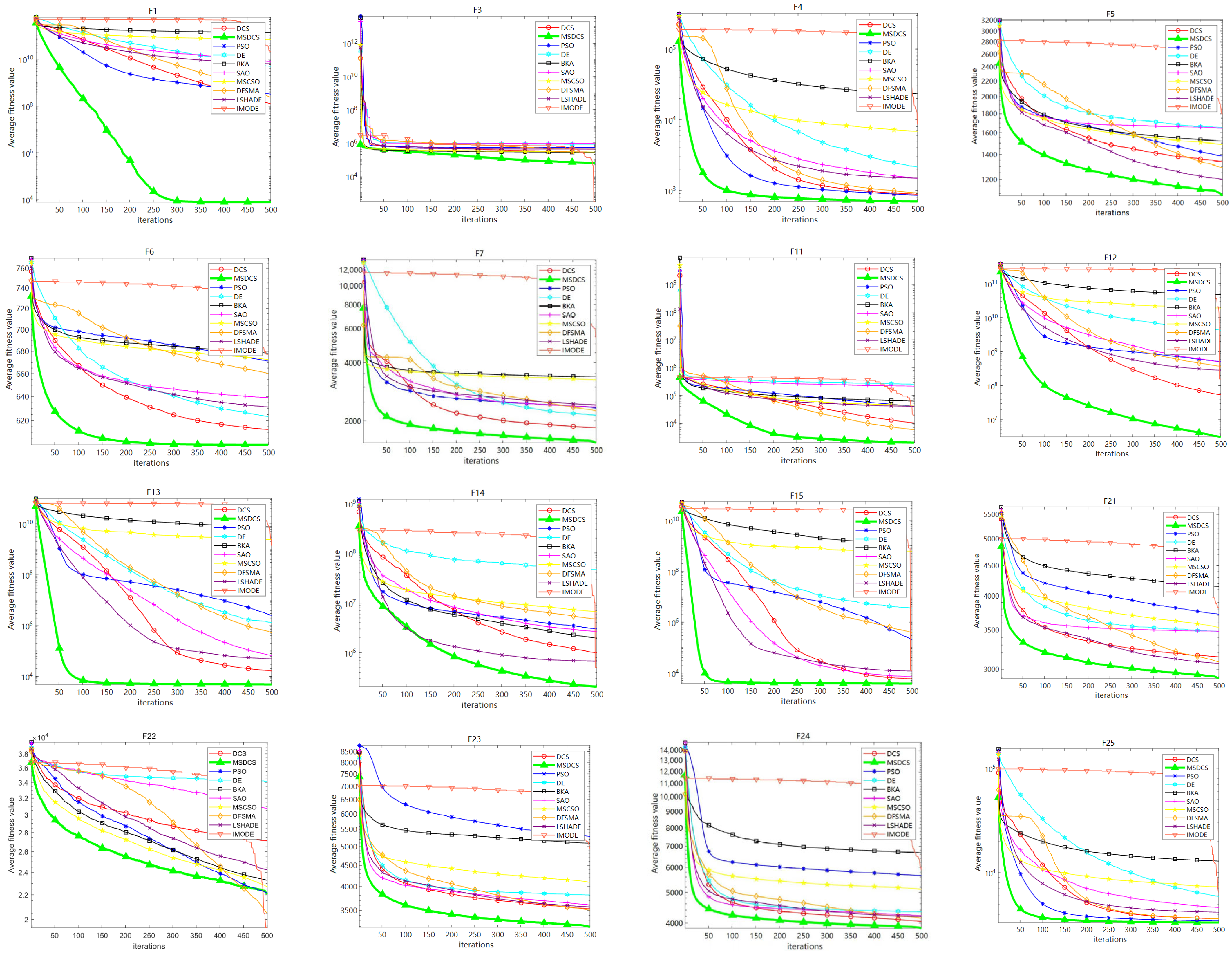
Table 6 shows the optimal value, mean, and standard deviation of the MSDCS obtained on 100 dimensions, as well as other comparison algorithms, for the 29 test functions of the CEC2017 test set. The results show that the MSDCS obtained three best results in single-peak functions (F1 and F3); fourteen best results in multi-peak functions (F4–F10); twenty-eight best results in hybrid functions (F11–F20); and fourteen best results in combined functions (F21–F30), which are significantly better than the original algorithm and the other compared algorithms. The test results indicate that the MSDCS exhibits a rapid convergence rate, strong optimization potential, and improved local escape capacity. The iterative convergence behavior of a representative set of 16 functions selected from the test set is shown in Figure 2. It demonstrates that the MSDCS converges faster than other algorithms in the early iteration phase and has much higher convergence accuracy in the later period. In conclusion, the convergence curves in Figure 2 and the experimental findings in Table 6 both confirm the efficiency of the MSDCS, which outperforms other algorithms in the optimization-seeking process.

Figure 2 shows the iterative convergence behavior of the 16 typical functions chosen from the test set. The MSDCS exhibits superior convergence speed and accuracy compared to other methods. Although F3’s convergence accuracy for the MSDCS is not as excellent as that of IMODE, its convergence speed surpasses that of the other algorithms. Functions F4–F7 have several peaks. The figure demonstrates that the MSDCS performs better than the other algorithms in terms of both convergence speed and accuracy. This suggests that other comparison algorithms often become stuck in local optima. Functions F11–F15 are hybrid functions, and MSDCS’s superior performance demonstrates its adaptability in complex environments. Although the convergence accuracy of the MSDCS in F22 is not as high as that of DFSMA and IMODE, it is still higher than that of the other algorithms in F22, with the MSDCS achieving the highest accuracy in other functions. When optimizing high-dimensional functions, the other algorithms usually fall into local optima, which slows the convergence speed. In contrast, the MSDCS usually obtains a better initial population by adopting a good point set and oppositional learning strategy and then finds the potential optimal solutions through the adaptive fitness–distance balanced reset strategy and the vertical and horizontal crossover, thus jumping out of the local optimum and finally converging to the global optimum to improve the optimization accuracy. It is worth mentioning that the MSDCS outperformed the original DCS, which also had favorable results, indicating the success of the three improvement methods introduced in the present study. In summary, the experimental results in Table 6 and the convergence curves in Figure 2 verify the effectiveness of the MSDCS algorithm, which has a better capability for finding optimization than the other comparison algorithms.

5.3. Wilcoxon Rank-Sum Test and Friedman Test

To further confirm the performance of the MSDC, the Wilcoxon rank-sum test is utilized to determine whether the algorithm is substantially different from the other comparable methods at a 5% significance level. The symbols “+”, “−”, and “=” show that the MSDCS outperforms, underperforms, or is equivalent to the other compared algorithms. The results are shown in

Table 7. The results of the Wilcoxon rank-sum test and the Friedman test.

	MSDCS	DCS	PSO	DE	BKA	SAO	MSCSO	DFSMA	LSHADE	IMODE
+/−/=	0/0/0	28/1/0	26/1/2	29/0/0	28/0/1	27/2/0	27/1/1	29/0/0	28/0/1	24/4/1
Ranking mean	1.79	4.09	5.57	8.05	8.52	5.48	7.36	4.36	4.59	5.19
Ranking	1	2	7	9	10	6	8	3	4	5

, where the MSDCS performs better than the other compared algorithms in most cases out of the 29 tested functions, thus indicating that the algorithm has a better ability to find an optimal solution. Friedman’s test, which is an analysis of variability in problem solving for a variety of methods, is used to obtain a comparison of the strengths and weaknesses of the algorithms by calculating the average rankings of the compared algorithms. As shown in Table 7, the MSDCS is ranked 1, suggesting that it has the best overall performance among the 29 functions evaluated.

6. MSDCS Algorithm for Optimizing the Agricultural UAV Path Planning Problem

6.1. Problem Modeling

UAVs are frequently used in agricultural production for tasks like irrigation, fertilizer and pesticide spraying, field monitoring, and other tasks. To ensure that the agricultural UAV can accomplish the mission successfully, reasonable flight route planning must be performed. In complex terrain, agricultural UAVs need to fly from the starting point to the target point following the result of path planning. During flight, agricultural UAVs may confront topographical barriers, weather hazards, radar scanning zones, and other obstacles, as well as limits such as fuel consumption, maximum climb capacity, and maximum turning capacity. To enable the safe and coordinated flight of agricultural UAVs, path planning algorithms need to connect the best route between the start and target points.

The agricultural UAV is assumed to maintain a predetermined flight speed, which reduces the path planning problem to a static polyline planning problem. The cost function $F\left(X_i\right)$ for agricultural UAV path planning is defined by computing the range length cost, flying altitude cost, threat cost, and smoothing cost using Equation (25) to satisfy the operational needs as follows:

$$F\left(X_i\right)={\displaystyle \sum }_{k=1}^4{b}_k{F}_k\left(X_i\right)$$

(25)

where the list of $n$ waypoints that the agricultural UAV is supposed to fly is represented by the decision variable $X_i$. $F_k$ is the $k$th cost function, and $b_k$ is the weight of each cost function. The descriptions of each cost function are given below.

6.2. Voyage Length Cost

The flight path length of agricultural UAVs should be as low as feasible to minimize fuel consumption. The agricultural UAV is controlled from a ground control station, and its flight route $X$ is represented as a list of $n$ waypoints that the agricultural UAV must travel, with each path point corresponding to the coordinates $P_{ij}=\left(x_{ij},y_{ij},z_{ij}\right)$. The path length is derived as the sum of several segments, with each segment’s length calculated using the Euclidean distance between two nodes. The voyage length cost $F_1$ is computed by Equation (26) as follows:

$$F_1\left(X_i\right)={\displaystyle \sum }_{j=1}^{n-1}\begin{array}{c}\Vert \underset{P_{ij}{P}_{i,j+1}}{\to }\Vert \end{array}$$

(26)

6.3. Threat Cost

Path planning for agricultural UAVs must not only optimize path length but also assure safe operation by avoiding no-fly zones known as hazard zones (e.g., radar detection, air defense equipment attacks, weather threats, etc.). The threat environment is abstracted, and the threat region is a cylinder with a fixed radius. The agricultural UAV is intended to successfully avoid the threat region and complete the flight. Figure 3 illustrates the abstracted threat region.

The obstacle in Figure 3 is represented by the green area; $K$ is the number of all obstacles where a threat exists, and its radius is indicated by $R_k$. The collision area, or white area, is represented by $D$, which is the agricultural UAV’s diameter, and $d_k$ indicates the vertical distance from the given path (from $P_{ij}$ to $P_{i,j+1}$) to the obstacle’s center. The hazardous area, or red area $S$, is determined by the agricultural UAV’s localization accuracy and the flight environment. If the agricultural UAV is in a static area with a strong signal, the value of $S$ might be a few tens of meters; if there are moving things nearby or the signal is weak, it might be more than a hundred meters. $T_k$ is the threat cost of path $P_{ij}$ to $P_{i,j+1}$ for a path whose threat cost $F_2$ is calculated by Equations (27) and (28) as follows:

$$F_2\left(X_i\right)={\displaystyle \sum }_{j=1}^{n-1}{\displaystyle \sum }_{k=1}^K{T}_k(\begin{array}{c}\underset{P_{ij}{P}_{i,j+1}}{\to }\end{array})$$

(27)

$$T_k\left(\begin{array}{c}\underset{P_{ij}{P}_{i,j+1}}{\to }\end{array}\right)=\left\{\begin{array}{c}0, if d_k>S+D+R_k\\ \left(S+D+R_k\right)-d_k, if\\ \infty , if d_k\le D+R_k\end{array}\right.D+R_k<d_k\le S+D+R_k$$

(28)

6.4. High Cost

An agricultural UAV is often limited to a flight altitude between the minimum altitude ($h_{min}$) and the maximum altitude ($h_{max}$). The UAV’s altitude relative to the ground is represented by the variable $h_{ij}$. The altitude cost $H_{ij}$ for each waypoint is added up to obtain the altitude cost $F_3$. It is evident that the altitude cost will punish values that are outside of range while maintaining the average altitude. High costs are shown by Equations (29) and (30).

$$F_3\left(X_i\right)={\displaystyle \sum }_{j=1}^n{H}_{ij}$$

(29)

$$H_{ij}=\left\{\begin{array}{c}\left|h_{ij}-{\displaystyle \frac{h_{min}+h_{max}}{2}}\right|, if h_{min}\le h_{ij}\le h_{max}\\ \infty , otherwise\end{array}\right.$$

(30)

6.5. Smoothing Cost

The flight angle control parameters for agricultural UAVs primarily involve the horizontal steering angle and vertical pitch angle. The trajectory planning model needs to make sure that these two parameters meet the agricultural UAV’s actual angle limits in order to produce feasible flight paths. The horizontal steering angle is an angle between two successive path segments projected on the horizontal plane $Oxy$ and is represented by ${\varnothing }_{ij}$, and the projections of $P_{ij}$ and $P_{i,j+1}$ are $P_{ij}^{\prime }$ and $P_{i,j+1}^{\prime }$. The angle between two successive path segments projected on the $Z$-axis is known as the vertical pitch angle, or ${\phi }_{ij}$. The penalization coefficients for the vertical pitch angle, $Z_{i,j+1}-Z_{ij}$, denote the height difference between two points and the horizontal steering angle, which are $a_1$ and $a_2$, respectively. Based on these values, the smoothing cost can be computed by Equations (31)–(33) as follows:

$$F_4\left(X_i\right)=a_1{\displaystyle \sum }_{j=1}^{n-2}{\varnothing }_{ij}+a_2{\displaystyle \sum }_{j=1}^{n-1}\left|{\phi }_{ij}-{\phi }_{i,j-1}\right|$$

(31)

$${\varnothing }_{ij}=\arctan \left({\displaystyle \frac{\Vert \overrightarrow{P_{ij}^{\prime }{P}_{i,j+1}^{\prime }}\times \overrightarrow{P_{i,j+1}^{\prime }{P}_{i,j+2}^{\prime }}\Vert }{\overrightarrow{P_{ij}^{\prime }{P}_{i,j+1}^{\prime }}.\overrightarrow{P_{i,j+1}^{\prime }{P}_{i,j+2}^{\prime }}}}\right)$$

(32)

$${\phi }_{ij}=\arctan \left({\displaystyle \frac{Z_{i,j+1}-Z_{ij}}{\Vert \overrightarrow{P_{ij}^{\prime }{P}_{i,j+1}^{\prime }}\Vert }}\right)$$

(33)

6.6. Simulation Experiment

6.6.1. Environmental Modeling and Parameterization

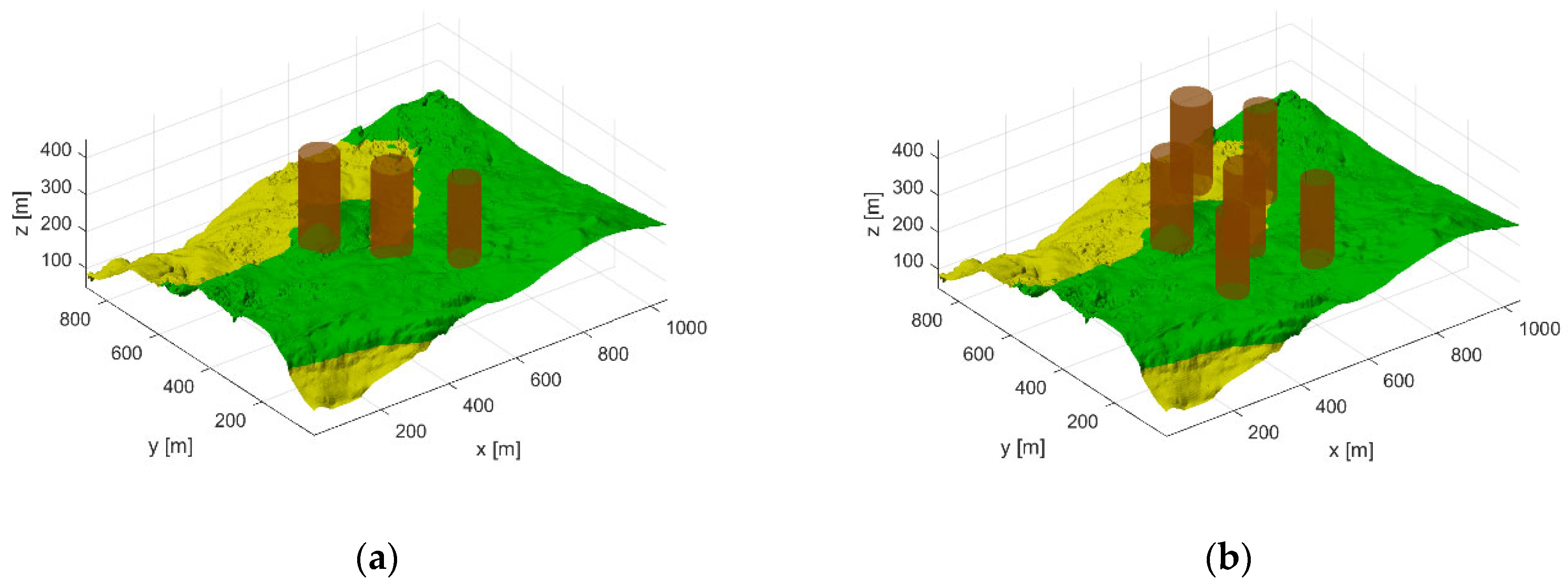
To further test the MSDCS’s performance in the agricultural UAV route planning problem, different threats are included to mimic various complicated terrains, and two terrains are constructed for path planning, as shown in Figure 4. In these scenarios, the number and location of threats (indicated by the brown columns) were chosen based on different levels of complexity, with Figure 4a showing a terrain map with a lower level of complexity and Figure 4b showing a terrain map with a higher level of complexity. For comparison, all algorithms were implemented with the same parameters: a population size of 30, 300 iterations, waypoints set to 10, the beginning position of the agricultural UAV (200, 100, 150), and the target position (800, 800, 150). For each comparison, all algorithms are performed ten times to determine the optimal, mean, and standard deviation.

6.6.2. Scenario One

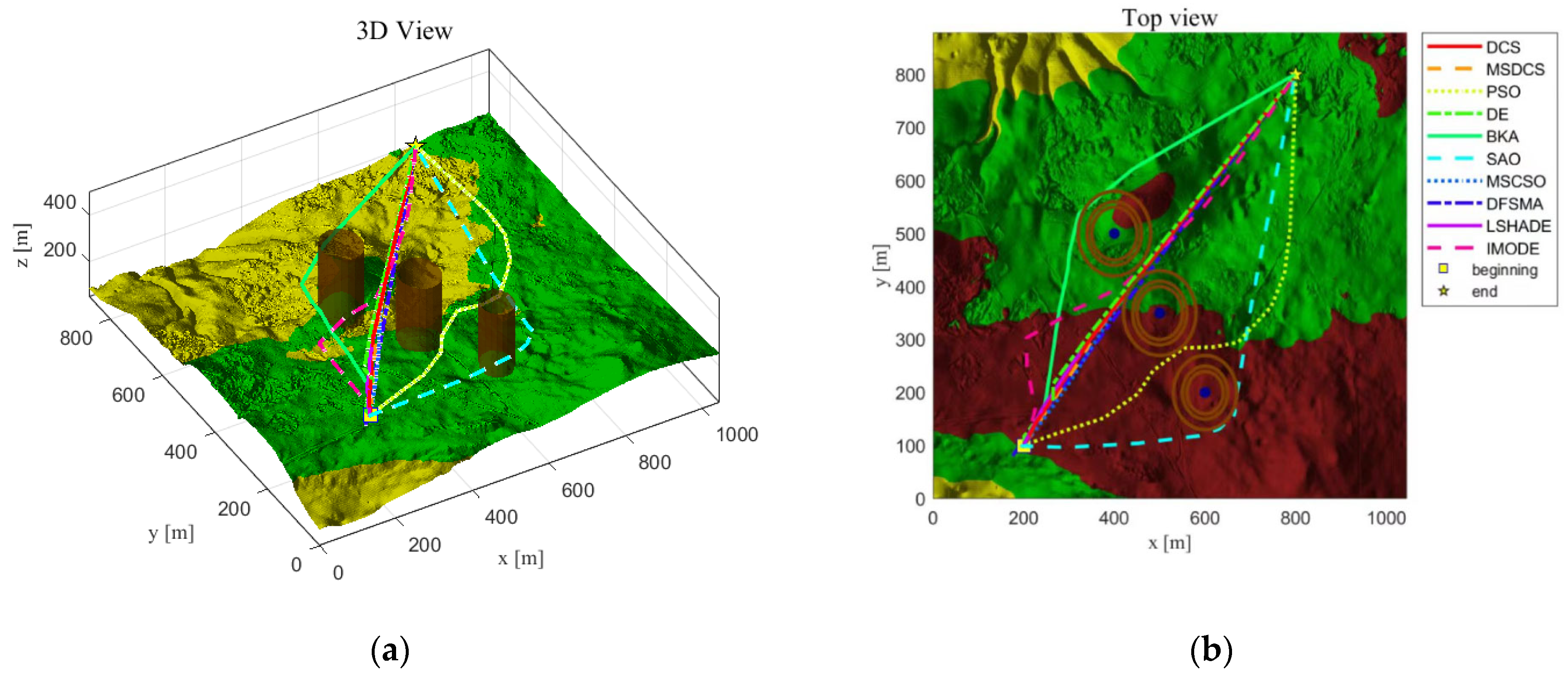
Figure 5 depicts the agricultural UAV flight trajectory maps of the MSDCS and other comparative algorithms. Figure 5a depicts the flight paths of all the algorithms in a 3D map, and to better observe the courses of the algorithms, the 3D map is converted into a 2D top view, as shown in Figure 5b. Most algorithms can discover a flight path from the origin to the destination; however, the pathways planned by the PSO, SAO, BKA, and IMODE have excessively wide steering angles, which can easily cause collisions. The MSDCS’s path can successfully avoid dangers and identify the flight path from the starting point to the target, while the agricultural UAV’s flight curve is reasonably smooth and approximates a straight flight.

The convergence curves of the optimal costs of several path planning algorithms are provided in Figure 6 to help visualize the effects of each algorithm more clearly. The MSDCS converges more quickly and with greater convergence accuracy than the other compared algorithms. The MSDCS outperforms the other algorithms in terms of optimal cost, average fitness value, and standard deviation (see

Table 8. The index data of simple terrain.

	MSDCS	DCS	PSO	DE	BKA	SAO	MSCSO	DFSMA	LSHADE	IMODE
cost	9.26 × 103	9.28 × 103	1.31 × 104	9.65 × 103	1.03 × 104	1.15 × 104	9.34 × 103	1.10 × 104	9.31 × 103	2.54 × 104
av	9.27 × 103	9.33 × 103	1.15 × 104	9.67 × 103	9.67 × 103	1.07 × 104	9.32 × 103	1.09 × 104	9.75 × 103	2.35 × 104
std	5.07	5.23 × 10	8.23 × 102	1.59 × 102	4.41 × 102	5.30 × 102	4.13 × 10	7.53 × 10	6.46 × 102	2.14 × 103

).

6.6.3. Scenario Two

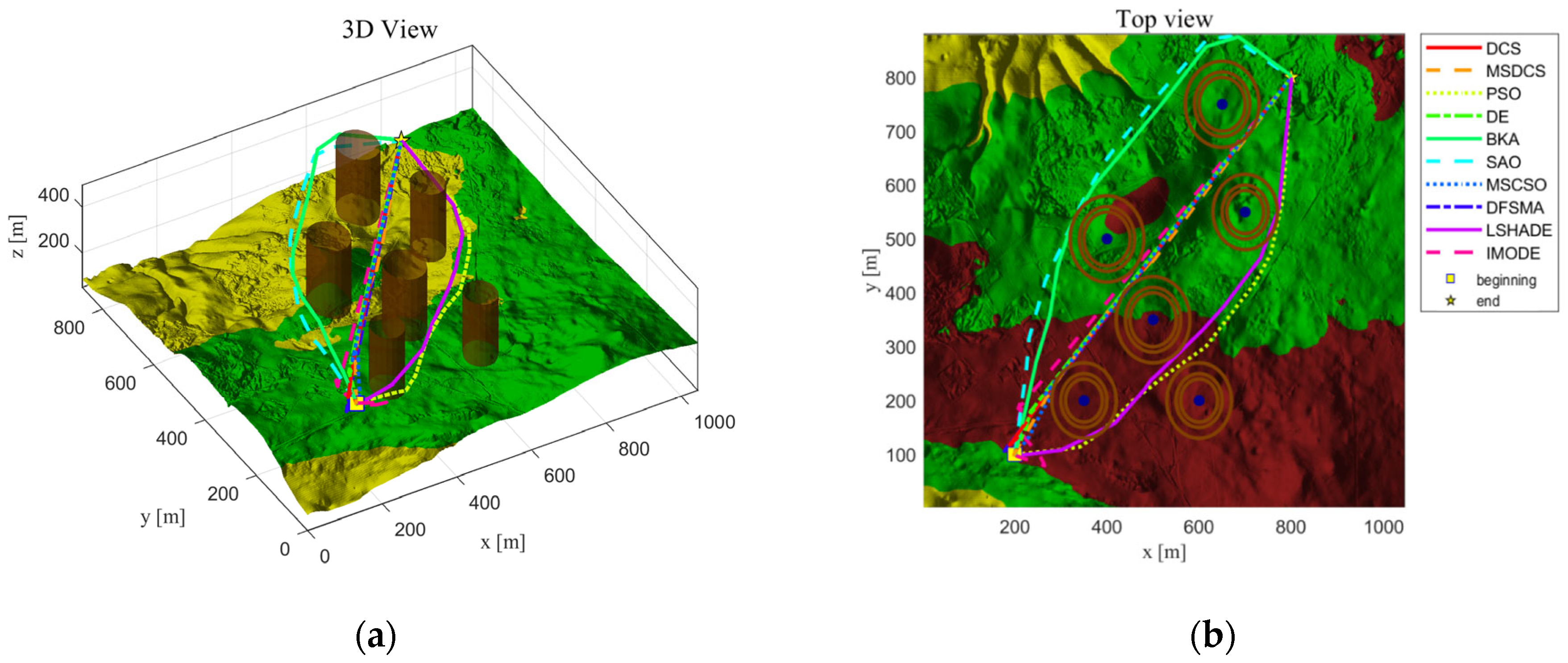
Figure 7 demonstrates that the MSDCS can still generate substantially realistic smoothed pathways in difficult settings. In contrast, the SAO and BKA opt to bypass the threat objects on the left, while the PSO and LSHADE choose to bypass the threat objects on the right, resulting in high costs for the agricultural UAV. Additionally, the flight routes of the remaining algorithms are not as sensible and practicable as those of the MSDCS. Figure 8 shows a cost function curve. Although most algorithms are comparable,

Table 9. The index data of complex terrain.

	MSDCS	DCS	PSO	DE	BKA	SAO	MSCSO	DFSMA	LSHADE	IMODE
cost	9.31 × 103	9.59 × 103	1.23 × 104	9.77 × 103	1.14 × 104	1.23 × 104	9.74 × 103	1.20 × 104	1.10 × 104	2.88 × 104
av	9.30 × 103	9.59 × 103	1.23 × 104	1.07 × 104	1.06 × 104	1.12 × 104	9.87 × 103	1.20 × 104	9.99 × 103	2.87 × 104
std	1.17 × 10	9.94 × 10	2.07 × 103	5.49 × 102	9.71 × 102	7.09 × 102	6.10 × 102	3.66 × 10	6.47 × 102	2.94 × 103

shows that the MSDCS has a lower cost price, a lower average fitness value, and is more stable.

7. Conclusions

The simulation experiments based on the CEC2017 test set in Section 5 lead to the conclusion that the MSDCS has a fast convergence speed and high accuracy compared to the other nine comparison algorithms, and the comprehensive performance of the MSDCS ranks first in Friedman’s test, which proves the effectiveness of the improved algorithm. Section 6 applies the improved algorithms to the agricultural UAV path planning problem. It can be seen in Figure 5, Figure 6, Figure 7 and Figure 8 that the PSO, SAO, BKA, IMODE, and LSHADE algorithms have poorer performance in solving the agricultural UAV path planning, and the flight paths obtained are prone to incur high flight costs and even higher risks during the flight process, whereas the MSDCS has a faster convergence speed and higher convergence accuracy. Compared to other algorithms, the MSDCS can obtain better flight paths for agricultural UAVs with a safer flight process, thus reducing the flight cost. Table 8 and Table 9 show that the MSDCS produces high-quality solutions in agricultural UAV path planning in both simple and complex scenarios with good stability.

This study not only confirms the efficacy of the MSDCS but also its practical worth in agricultural UAV path planning. The comparative study demonstrates that the MSDCS exhibits notable superiority in effectively navigating various intricate situations. When compared to the classical PSO method, the PSO exhibits a higher rate of convergence. However, it demonstrates limited stability and adaptability in the presence of impediments. The MSDCS, in this study, demonstrates superior capability in guaranteeing that agricultural UAVs locate the most advantageous route while evading obstacles, hence enhancing the quality and efficiency of UAV flight pathways for path planning.

The cost function of agricultural UAV path planning is flexible, encompassing factors like fuel consumption and collision risk. In the future, the algorithm can be modified to achieve more comprehensive optimization of agricultural UAV path planning. This will cater to a variety of agricultural application scenarios, ensuring the efficient and safe operation of agricultural UAVs. Furthermore, it will further advance the development of agricultural UAVs in the field of agriculture.

8. Summary

For the agricultural UAV path planning problem, a multi-strategy improved differentiated creative search algorithm is proposed. The MSDCS employs the good point set and the oppositional learning strategy to increase the diversity of the population and improve the quality of the solution; the adaptive fitness–distance balanced reset strategy prompts the low performers to converge to the optimal solution region. Additionally, the vertical and horizontal crossover strategy with random dimensions is proposed to help the algorithm jump out of the local optimum and improve the convergence accuracy.

To demonstrate the MSDCS’s effectiveness, 29 test functions from the CEC2017 test set are used for comparison experiments with the original algorithms, the classical algorithms, the most recent modified algorithms, and the competition algorithms. The experimental results reveal that the MSDCS outperforms the other comparative algorithms in terms of convergence speed, accuracy, and stability. Further validation is performed using the Wilcoxon rank-sum test and the Friedman test, and the findings confirmed the MSDCS’s excellent performance.

Two sets of experiments are conducted using relatively simple terrain maps and relatively complex terrain maps to test the performance of the MSDCS in agricultural UAV path planning problems. The simulation experiments show that the MSDCS algorithm can converge quickly and generate efficient and collision-free agricultural UAV flight paths in both simple and complex scenarios, which verifies the applicability and superiority of the MSDCS.

References

1. Plessen, M. Path Planning for Spot Spraying with UAVs Combining TSP and Area Coverages. arXiv 2024, arXiv:2408.08001. [Google Scholar]
2. Hafeez, A.; Husain, M.A.; Singh, S.P.; Chauhan, A.; Khan, M.T.; Kumar, N.; Chauhan, A.; Soni, S.K. Implementation of drone technology for farm monitoring & pesticide spraying: A review. Inf. Process. Agric. 2023, 10, 192–203. [Google Scholar] [CrossRef]
3. Li, W.; Liu, C.; Yang, Y.; Awais, M.; Li, W.; Ying, P.; Ru, W.; Cheema, M.J.M. A UAV-aided prediction system of soil moisture content relying on thermal infrared remote sensing. Int. J. Environ. Sci. Technol. 2022, 19, 9587–9600. [Google Scholar] [CrossRef]
4. Budiharto, W.; Irwansyah, E.; Suroso, J.S.; Chowanda, A.; Ngarianto, H.; Gunawan, A.A.S. Mapping and 3D modelling using quadrotor drone and GIS software. J. Big Data 2021, 8, 48. [Google Scholar] [CrossRef]
5. Gugan, G.; Haque, A. Path Planning for Autonomous Drones: Challenges and Future Directions. Drones 2023, 7, 169. [Google Scholar] [CrossRef]
6. Xu, D.; Qian, H.; Zhang, S. An Improved RRT*-Based Real-Time Path Planning Algorithm for UAV. In Proceedings of the 2021 IEEE 23rd Int Conf on High Performance Computing & Communications; 7th Int Conf on Data Science & Systems; 19th Int Conf on Smart City; 7th Int Conf on Dependability in Sensor, Cloud & Big Data Systems & Application (HPCC/DSS/SmartCity/DependSys), Haikou, China, 20–22 December 2021; pp. 883–888. [Google Scholar] [CrossRef]
7. Moon, S.; Oh, E.; Shim, D.H. An Integral Framework of Task Assignment and Path Planning for Multiple Unmanned Aerial Vehicles in Dynamic Environments. J. Intell. Robot. Syst. 2013, 70, 303–313. [Google Scholar] [CrossRef]
8. McCall, J. Genetic algorithms for modelling and optimisation. J. Comput. Appl. Math. 2005, 184, 205–222. [Google Scholar] [CrossRef]
9. Dorigo, M.; Di Caro, G. Ant colony optimization: A new meta-heuristic. In Proceedings of the 1999 Congress on Evolutionary Computation-CEC99 (Cat. No. 99TH8406), Washington, DC, USA, 6–9 July 1999; pp. 1470–1477. [Google Scholar] [CrossRef]
10. Mirjalili, S.; Mirjalili, S.M.; Lewis, A. Grey Wolf Optimizer. Adv. Eng. Softw. 2014, 69, 46–61. [Google Scholar] [CrossRef]
11. Heidari, A.A.; Mirjalili, S.; Faris, H.; Aljarah, I.; Mafarja, M.; Chen, H. Harris hawks optimization: Algorithm and applications. Future Gener. Comput. Syst. 2019, 97, 849–872. [Google Scholar] [CrossRef]
12. Mirjalili, S.; Lewis, A. The Whale Optimization Algorithm. Adv. Eng. Softw. 2016, 95, 51–67. [Google Scholar] [CrossRef]
13. Mirjalili, S. SCA: A Sine Cosine Algorithm for solving optimization problems. Knowl.-Based Syst. 2016, 96, 120–133. [Google Scholar] [CrossRef]
14. Li, S.; Chen, H.; Wang, M.; Heidari, A.A.; Mirjalili, S. Slime mould algorithm: A new method for stochastic optimization. Future Gener. Comput. Syst. 2020, 111, 300–323. [Google Scholar] [CrossRef]
15. Chen, Q.; He, Q.; Zhang, D. UAV Path Planning Based on an Improved Chimp Optimization Algorithm. Axioms 2023, 12, 702. [Google Scholar] [CrossRef]
16. Zhang, W.; Zhang, S.; Wu, F.; Wang, Y. Path Planning of UAV Based on Improved Adaptive Grey Wolf Optimization Algorithm. IEEE Access 2021, 9, 89400–89411. [Google Scholar] [CrossRef]
17. Wang, Q.; Xu, M.; Hu, Z. Path Planning of Unmanned Aerial Vehicles Based on an Improved Bio-Inspired Tuna Swarm Optimization Algorithm. Biomimetics 2024, 9, 388. [Google Scholar] [CrossRef]
18. Tan, L.; Zhang, H.; Shi, J.; Liu, Y.; Yuan, T. A robust multiple Unmanned Aerial Vehicles 3D path planning strategy via improved particle swarm optimization. Comput. Electr. Eng. 2023, 111, 108947. [Google Scholar] [CrossRef]
19. He, Y.; Wang, M. An improved chaos sparrow search algorithm for UAV path planning. Sci. Rep. 2024, 14, 366. [Google Scholar] [CrossRef]
20. Yu, X.; Jiang, N.; Wang, X.; Li, M. A hybrid algorithm based on grey wolf optimizer and differential evolution for UAV path planning. Expert Syst. Appl. 2023, 215, 119327. [Google Scholar] [CrossRef]
21. Zhu, D. Human memory optimization algorithm: A memory-inspired optimizer for global optimization problems. Expert Syst. Appl. 2024, 237, 121597. [Google Scholar] [CrossRef]
22. Duankhan, P.; Sunat, K.; Chiewchanwattana, S.; Nasa-ngium, P. The Differentiated Creative search (DCS): Leveraging Differentiated knowledge-acquisition and Creative realism to address complex optimization problems. Expert Syst. Appl. 2024, 252, 123734. [Google Scholar] [CrossRef]
23. Geoscience Australia. Digital Elevation Model (DEM) of Australia Derived from LiDAR 5 Metre Grid; Geoscience Australia: Canberra, Australia, 2015. [CrossRef]
24. Yang, W.; Xia, K.; Li, T.; Xie, M.; Song, F. A Multi-Strategy Marine Predator Algorithm and Its Application in Joint Regularization Semi-Supervised ELM. Mathematics 2021, 9, 291. [Google Scholar] [CrossRef]
25. Kiefer, J.C. On large deviations of the empiric D. F. of vector chance variables and a law of the iterated logarithm. Pacific J. Math. 1961, 11, 649–660. [Google Scholar] [CrossRef]
26. Deng, L.; Liu, S. An enhanced slime mould algorithm based on adaptive grouping technique for global optimization. Expert Syst. Appl. 2023, 222, 119877. [Google Scholar] [CrossRef]
27. Kennedy, J.; Eberhart, R. Particle swarm optimization. In Proceedings of the ICNN’95—International Conference on Neural Networks, Perth, WA, Australia, 27 November–1 December 1995; Volume 4, pp. 1942–1948. [Google Scholar] [CrossRef]
28. Storn, R. Differential Evolution—A Simple and Efficient Heuristic for Global Optimization over Continuous Spaces. J. Glob. Optim. 1997, 11, 341–359. [Google Scholar] [CrossRef]
29. Wang, J.; Wang, W.; Hu, X.; Qiu, L.; Zang, H. Black-winged kite algorithm: A nature-inspired meta-heuristic for solving benchmark functions and engineering problems. Artif. Intell. Rev. 2024, 57, 98. [Google Scholar] [CrossRef]
30. Deng, L.; Liu, S. Snow ablation optimizer: A novel metaheuristic technique for numerical optimization and engineering design. Expert Syst. Appl. 2023, 225, 120069. [Google Scholar] [CrossRef]
31. Wu, D.; Rao, H.; Wen, C.; Jia, H.; Liu, Q.; Abualigah, L. Modified Sand Cat Swarm Optimization Algorithm for Solving Constrained Engineering Optimization Problems. Mathematics 2022, 10, 4350. [Google Scholar] [CrossRef]
32. Hu, J.; Gui, W.; Heidari, A.A.; Cai, Z.; Liang, G.; Chen, H.; Pan, Z. Dispersed foraging slime mould algorithm: Continuous and binary variants for global optimization and wrapper-based feature selection. Knowl.-Based Syst. 2022, 237, 107761. [Google Scholar] [CrossRef]
33. Tanabe, R.; Fukunaga, A.S. Improving the search performance of SHADE using linear population size reduction. In Proceedings of the 2014 IEEE Congress on Evolutionary Computation (CEC), Beijing, China, 6–11 July 2014; pp. 1658–1665. [Google Scholar] [CrossRef]
34. Fan, J.; Xiong, S.; Wang, J.; Gong, C. IMODE: Improving Multi-Objective Differential Evolution Algorithm. In Proceedings of the 2008 Fourth International Conference on Natural Computation, Jinan, China, 18–20 October 2008; pp. 212–216. [Google Scholar] [CrossRef]
Figure 1. A comparison diagram of random initialization and good point set initialization. (a) Random initialized distribution plot. (b) Distribution of the initialization based on the set of good points.
Machines 12 00591 g001
Figure 2. Convergence curves for 16 functions selected from the CEC2017 test set.
Machines 12 00591 g002
Figure 3. Images of the threat area.
Machines 12 00591 g003
Figure 4. Topographic maps of different complexities. (a) A topographic map with a low number of threats. (b) A topographic map with a high number of threats.
Machines 12 00591 g004
Figure 5. The flight path diagram of the UAV in scenario one. (a) The flight path in a simple scenario. (b) A top view of the flight path in a simple scenario.
Machines 12 00591 g005
Figure 6. Cost function curves for all algorithms.
Machines 12 00591 g006
Figure 7. The flight path diagram of the UAV in scenario two. (a) The flight path in a complex scenario. (b) A top view of the flight path in a complex scenario.
Machines 12 00591 g007
Figure 8. Cost function curves for all algorithms.
Machines 12 00591 g008