Abstract
This paper presents a novel approach for extracting 3D weld point information using a two-stage deep learning pipeline based on readily available 2D RGB cameras. Our method utilizes YOLOv8s for object detection, specifically targeting vertices, followed by semantic segmentation for precise pixel localization. This pipeline addresses the challenges posed by low-contrast images and complex geometries, significantly reducing costs compared with traditional 3D-based solutions. We demonstrated the effectiveness of our approach through a comparison with a 3D-point-cloud-based method, showcasing the potential for improved speed and efficiency. This research advances the field of automated welding by providing a cost-effective and versatile solution for extracting key information from 2D images.
1. Introduction
The shipbuilding industry is heavily reliant on efficient and precise construction techniques. Welding complex double-hull structures, which are crucial for ship safety and stability, often presents significant challenges when using traditional manual methods. This has become a bottleneck in the development of the modern shipbuilding industry [1].
Double-hull structures, which are characterized by intricate networks of intersecting plates and stiffeners, create a visually complex environment that complicates weld point identification. This paper proposes a novel approach designed to address this challenge by leveraging robotic welding coupled with automated weld point extraction using readily available and cost-effective 2D cameras. To evaluate the effectiveness of our approach, we compared its performance in terms of the processing time and accuracy against a system that utilized 3D cameras.
1.1. Background
Automated weld point extraction for robotic welding has shown promise, but limitations persist for complex structures with multiple welding joints. Existing robotic welding systems, like “Dandy” [2], utilize robotic arms to automate the welding of double-hull structures in ships, but often rely on pre-programmed welding paths. This requires significant manual input and limits their adaptability to complex geometries.
Traditional methods also suffer from a lengthy setup and programming times due to the manual identification of weld points within the complex double-hull structure. Furthermore, while 3D sensors offer high accuracy in weld point detection, their high cost and complex data processing limit their widespread adoption in the shipbuilding industry.
1.2. Related Work
A variety of approaches were suggested for the feature extraction of weld joints and initial weld points from point clouds. Dinham [3] generated point clouds from stereo camera sensors to extract straight-line weld joints for path planning. Zhang [4] and Gao [5] employed point cloud data to detect and extract initial welding positions, with Zhang concentrating on workpiece recognition and Gao on D-type weld seam extraction. Kim [6] focused on 3D point cloud segmentation, proposing a method for extracting multiple weld seams from RGB-depth images using point cloud registration to address occlusions. Yang [7] proposed methods for specific types of weld seams, achieving a high accuracy and robustness for intersecting pipes. Patil [8] presented a real-time weld seam extraction algorithm for 3D point clouds using a robot arm, which is a procedure similar to the one used in this study to extract the ground truth.
There were also studies on extracting initial weld points from 2D images. Wei [9] introduced a technique using image morphology but it was mainly used on planar setups. Liu [10] developed a precise initial weld position identification algorithm for fillet weld seams using laser vision technology.
Some approaches based on deep convolutional neural networks include those of Yang [11], who used YOLOv3 to locate weld seams on double-hull structures, and Li [12], who used YOLOv5 to detect the initial weld position of each piece.
While previous studies explored various techniques for initial weld point extraction, they often faced limitations in addressing the specific challenges posed by double-hull structures. These methods frequently focus on isolated structures with limited visual complexity, failing to generalize to real-world scenarios with multiple, overlapping welds, and intricate geometries.
1.3. Contribution
This paper proposes a novel approach designed to overcome the limitations of existing methods, enabling robust weld point identification, even in complex environments, like those found within double-hull ship structures. We utilized data obtained from a cost-effective 2D RGB camera to train two neural networks. The first network extracts key features, such as vertices, from the image. The second network then leverages these features to perform semantic segmentation around the vertex, pinpointing the region of interest. This allows for extracting a precise pixel representing the initial weld point, which is used to calculate a 3D position related to the frame of the robotic arm.
To benchmark our 2D approach, we utilized a 3D camera to establish ground truth data and evaluate the processing time and accuracy of both methodologies. This research could enhance the capabilities of robotic welding systems, like Dandy, by providing a more cost-effective and efficient solution for weld point extraction.
2. Materials and Methods
This section details the methodology that was employed to calculate accurate 3D information from 2D cameras for robotic operations, specifically focusing on initial weld point localization. The main objective was to obtain accurate 3D positions related to the robot frame. Two primary pipelines based on 3D point cloud and 2D image processing were defined and compared for their efficiency in capturing, processing, and extracting data.
The software primarily consisted of programming languages such as C++17 and Python 3.10. To automate the data collection phase, the robot and camera were connected to a computer via an ROS (robot operating system) [13].
For the camera captures, Python ROS nodes were developed to save captures to files for later processing. The 3D point clouds were processed using the C++ library Point Cloud Library (PCL) [14], and the 2D captures were processed using YOLOv8 [15]. Bash shell scripts and the Jupyter Python framework were used for testing and generating the final data.
2.1. Framework
Figure 1 depicts our experimental setup, which featured a Fanuc 200id robotic arm with 6 degrees of freedom (dofs) mounted on an 800 mm wide table. This setup emulated a “Dandy-like” robotic system that can be used in shipyards. In real-world scenarios, these robots are typically maneuvered into position within a ship’s open block using a crane, as illustrated in Figure 2. Our table served as a surrogate for the ship’s framework, providing a stable base for the robot once it was positioned.
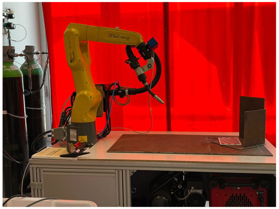
Figure 1.
Experimental setup for automated weld point extraction. Fanuc 200i-D robotic arm equipped with a welding torch and a dual 2D–3D RGB camera mounted on its end effector. A red welding curtain is visible behind the robot and workpiece.
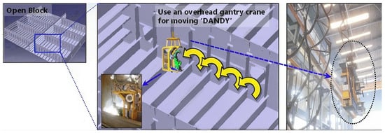
Figure 2.
Dandy moving capacity on open block [16]. Scientific Figure on ResearchGate. Available from: https://www.researchgate.net/figure/DANDY-a-fixed-welding-robot-used-by-Daewoo-Shipbuilding-Marine-Engineering-in-Korea_fig1_273632936 (accessed on 24 June 2024).
A camera, which was attached to the robot’s end effector, provided both point clouds and RGB images (Figure 3). This dual-sensor setup allowed for a comparative analysis between our novel 2D method and a conventional 3D-point-cloud-processing technique.
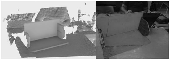
Figure 3.
The 3D point cloud (left); 2D image (right).
Our research utilized the Ensenso N35,which is a commercial 3D vision solution from IDS Imaging Development Systems GmbH based on active stereo vision technology. This versatile camera employs two cameras and a projector that projects a high-contrast pattern onto the scene, enhancing the 3D reconstruction of objects, particularly those with a low texture. Additionally, the Ensenso N35 incorporates a piezoelectric actuator to shift the projected rays linearly, further improving the 3D reconstruction of challenging surfaces, such as shiny, dark, or light-scattering objects. The Ensenso N35 is capable of generating both 3D point clouds and 2D images. The 3D point cloud, which consisted of approximately 1.3 million points, was represented in with a resolution of 1280 × 1024 pixels and exhibited a depth accuracy of 0.5–1 mm for working distances ranging from 0.27 to 3 m. The camera’s 2.3 MP sensor, with a resolution of 1936 × 1216 pixels, captured high-resolution 2D images alongside the 3D data. Additionally, the camera featured a focal length of 6–16 mm, allowing for flexible image capture at various distances.
Both the camera and the robot were connected to an MSI MS16-W2 laptop. This platform, featuring 64 GB of RAM and an Nvidia GeForce RTX 3050 CUDA graphics card, facilitated both the data processing and training of the deep learning models. This setup allowed for a direct comparison between our 2D solution and the 3D point cloud data acquired from the same camera, minimizing potential errors that arose from the extrinsic calibration.
While our research focused on vertex detection in the context of robotic welding, actual ship components are often massive, weighing several tons. This presents a significant challenge for testing in a university lab setting, as our facilities were limited to safely handling objects under 25 kg. To address this, we developed scaled-down versions of these pieces, each representing half of a real-world component, which would typically have two vertices. These scaled models measured between 200 and 400 mm in width and 100 mm and 200 mm in height, allowing us to test our algorithms in a controlled environment while maintaining the relevant geometric features. By focusing on a single vertex at a time, we could efficiently conduct experiments and gather data within the constraints of our laboratory.
Photos were typically captured with the robot positioned at the center of the 800 mm wide table. This positioning ensured consistent image framing and facilitated a standardized approach to data acquisition for both the 2D and 3D methods.
2.2. Two-Dimensional Feature Extraction
To accurately calculate the 3D position of the weld point from a 2D image, we needed to identify the corresponding pixel in the image. As our target weld points formed a U-shape, a vertex needed to be identified.
The U-shaped structures used in our experiments were fabricated from mild steel plates, which is a material that is widely employed in the shipbuilding industry. Mild steel exhibits desirable properties for shipbuilding applications, including a high tensile strength, which ensures structural integrity, and excellent welding characteristics, facilitating reliable joint creation [17]. Furthermore, the mild steel plates often possess a protective patina, which is a thin oxidized layer that forms naturally on the surface. This patina helps to mitigate issues related to shiny surfaces, which can pose challenges for vision-based systems due to specular reflections.
Due to the complexity of the scene, traditional edge-detection algorithms, like Canny or Bayesian filters, might fail to isolate the vertex reliably. Therefore, we employed a mixed pipeline approach, as illustrated in Figure 4, combining two supervised deep learning methods: object detection for vertex zone identification and semantic segmentation for precise pixel localization.

Figure 4.
Pixel extraction pipeline.
The process of detecting the initial weld point started with capturing an image of the workspace, which served as the foundation for the subsequent steps.
2.2.1. Object Detection
For robust and efficient vertex detection, we leveraged YOLO (You Only Look Once), which is a widely recognized real-time object detection system renowned for its speed, accuracy, and scalability. Our YOLO model was trained on a dataset specifically curated for this task, consisting of ship frame images annotated with bounding boxes that meticulously delineated the vertices. During the training process, the model learned to accurately predict the coordinates of these bounding boxes, effectively localizing the vertices for various points of interest (POIs).
We specifically employed YOLOv8, which is the most recent iteration of the YOLO family at the time of our research. This choice stemmed from its superior performance on our test machine, which was equipped with an Intel i7 processor and an Nvidia RTX Series GPU. YOLOv8 builds upon the advancements introduced in YOLOv5, incorporating further architectural and training enhancements to achieve improvements in both speed and accuracy. While YOLOv5 already demonstrated significant progress in real-time object detection, YOLOv8 takes a further step toward enabling efficient deployment on constrained edge devices. Notably, YOLOv8 focuses on the following:
- Increased inference speed: optimized architecture and model quantization techniques in YOLOv8 contribute to significantly faster inference, making it well-suited for real-time applications on edge devices with limited processing power;
- Reduced model size: YOLOv8’s efficient design results in smaller model sizes compared with YOLOv5, requiring less memory and storage, which are critical factors for deployment on edge devices.
This emphasis on high-inference speed and reduced model size in YOLOv8 strongly suggests its suitability for deployment on constrained edge devices, a crucial aspect for making our weld point detection system more accessible and practical in various industrial settings [18].
Table 1 summarizes the different YOLOv8 model variants, showcasing the trade-offs between model size, accuracy, speed, and computational complexity.

Table 1.
YOLOv8 detection models [19].
For our application, we opted for the YOLOv8s model, which is the second-smallest variant in the YOLOv8 lineup. This strategic choice balanced performance with computational efficiency. While larger models like YOLOv8m, YOLOv8l, or YOLOv8x might offer a marginally higher accuracy, their increased computational demands could pose challenges for deployment on resource-constrained hardware. YOLOv8s, on the other hand, provides a compelling blend of accuracy and speed, enabling reliable vertex detection, even in low-resolution images, while maintaining feasibility for real-time applications.
To train the YOLOv8s model, we curated a dataset that comprised images from real pieces combined with others taken in the lab, some with natural light and others with artificial light. We manually labeled 41 photographs, focusing on the vertex regions, and used Roboflow [20] to augment this dataset, resulting in a total of 95 images. The augmentation techniques applied included the following:
- Horizontal flips: mirroring the images horizontally to increase the variety of vertex orientations;
- Rotations: rotating images by ±15° to account for potential variations in camera orientation;
- Exposure adjustments: modifying the exposure by +10% and −10% to introduce robustness to different lighting conditions;
- Blurring: applying a Gaussian blur with a radius of up to 2.5 pixels to simulate slight defocusing or motion blur.
These data augmentation techniques played a crucial role in enhancing the model’s robustness, particularly in scenarios involving small object detection. By expanding the training dataset with diverse variations of the original images, the model learned to generalize better and becomes more resilient to changes in lighting, orientation, and image quality.
As this research represented a proof of concept, the dataset size was intentionally limited. However, for production-level deployments, the dataset can be readily expanded to further improve the model’s accuracy and generalizability. The dataset can be explored and downloaded at the following link: https://universe.roboflow.com/ml2d/ml2d (accessed on 24 June 2024).
The training was performed using the YOLO training pipeline, employing the following parameters:
- Image resolution: The input images were resized to 640 × 640 pixels, which is a commonly used resolution for YOLO models. This ensured a consistent input size for the model.
- Epochs: the model was trained for 75 epochs, which is a relatively small number to mitigate overfitting due to the limited dataset size.
- Batch size: A batch size of 16 was used during the training. This means that the model was updated after simultaneously processing 16 images. This parameter was based on the available resources. A larger batch size can improve the training speed, but it might require more memory.
- Learning rate: The learning rate was set to 0.01. This parameter controls how much the model’s weights are adjusted during each training iteration. A higher learning rate can lead to faster convergence, but it might result in oscillations or overshooting the optimal weights.
- Optimizer: The stochastic gradient descent (SGD) optimizer was employed. The SGD is a classic optimization algorithm that iteratively updates the model’s weights based on the gradient of the loss function.
Figure 5 shows the results after training. The training loss curves for the bounding box, classification, and confidence score prediction all decreased significantly over the 75 epochs, indicating that the model learned effectively. The model achieved a good performance with high precision (around 0.7), recall (around 0.6), and mAP scores (reaching approximately 0.55 for mAP50). This suggests that the trained model was capable of accurately detecting vertex regions within images.
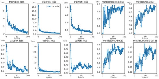
Figure 5.
Training curves and performance metrics for the YOLOv8s object detection model. The x-axis represents the training epochs (unitless), and the y-axis represents the loss values (unitless). The curves illustrate the model’s learning progress, with a significant decrease in loss and improvements in the precision, recall, and mAP50 scores, indicating effective training.
Once trained, the YOLOv8s model could be deployed to detect the vertex regions in new images. The predicted bounding box coordinates generated by the model were then used to crop the relevant regions, facilitating the next stage of semantic segmentation for precise pixel localization.
2.2.2. Semantic Segmentation
While the object detection model effectively identifies a bounding box encompassing the vertex, the vertex itself might be slightly offset from the center of this region. Furthermore, the workspace’s characteristics, including the grayscale camera and dark metal surfaces, can produce images with low contrast. This low contrast increases the risk of false positives when using traditional analytical methods. To address these challenges, we employed semantic segmentation, specifically on the cropped vertex regions.
Instead of segmenting the entire image, which could lead to extensive post-processing, we focused on the cropped region obtained from the object detection stage. This cropped region was a small image, typically around 50 × 50 or 12 × 12 pixels. We then scaled this cropped image to 640 × 640 pixels to match the input requirements of the semantic segmentation model. We annotated the pixels surrounding the vertex to train the semantic segmentation model. This focused approach, particularly in the context of low-contrast images, facilitated the pattern recognition and enhanced the segmentation accuracy.
The dataset, which is available at https://universe.roboflow.com/ml2d/sam_vertex (accessed on 24 June 2024), comprises images obtained from the previous object detection model applied to various pieces. Some of these images were further processed using the Segment Anything Model (SAM) [21].
To achieve optimal convergence in this training process, the semantic segmentation model required an extended training regimen of 250 epochs using the YOLO training pipeline. This training utilized the semantic segmentation model with the same learning rate, optimizer, and batch parameters as the object detection model.
The results of the semantic segmentation training can be seen in Figure 6. The figure displays training curves for a YOLO-based semantic segmentation model trained for 250 epochs to precisely locate vertices within cropped images. The curves show the training loss for the bounding box, segmentation, classification, and confidence score predictions. The x-axis represents the training epochs, and the y-axis represents the loss value (unitless).

Figure 6.
Training curves for the YOLO-based semantic segmentation. The x-axis represents the training epochs, and the y-axis represents the loss (unitless). The curves show a decreasing trend in loss across all tasks, indicating that the model effectively learned to identify vertices within cropped images.
As the training progressed over 200 epochs, significant decreases were observed in all loss curves, indicating that the model effectively learned to identify the vertex within the cropped image. This was further supported by the decrease in the loss related to the bounding box, segmentation, classification, and confidence score predictions, suggesting that the model learned to distinguish the vertex accurately from its surroundings.
2.2.3. Pixel Calculation
Once the vertex region was segmented, we pinpointed the precise vertex location by calculating the middle point of all segmented pixels. Figure 7 showcases the results of the 2D pipeline. The figure presents a series of four images for each of three different vertices, representing a progression through the pipeline.
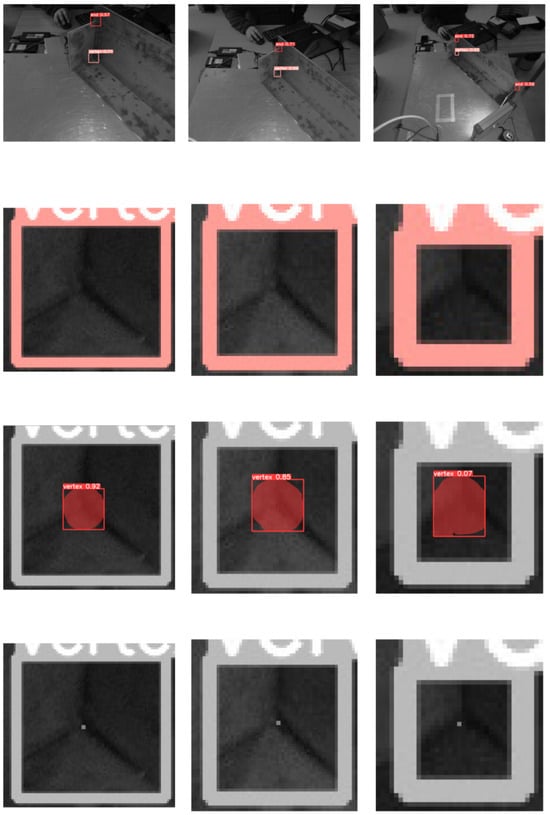
Figure 7.
Results of the 2D pipeline for vertex detection and localization. Each row shows the steps involved in processing a single vertex: original image with a bounding box, cropped region, semantic segmentation, and final pixel location.
- Image 1: the first image in each set shows the original image with the bounding box from the object detection stage, highlighting the detected vertex;
- Image 2: the second image shows the cropped area around the detected vertex, which was further processed by the semantic segmentation model;
- Image 3: the third image shows the result of the semantic segmentation, where the pixels corresponding to the vertex are highlighted in red;
- Image 4: the fourth image shows the final pixel location calculated from the semantic segmentation, as represented by a small white circle in the center of the segmented area.
The figure demonstrates the effectiveness of our 2D pipeline in accurately identifying and localizing the vertex points, which were crucial for determining the initial weld point. The images clearly show how the pipeline operates, from detecting the vertex in the full image to selecting the precise pixel location through a series of processing steps. As can be seen from left to right, as the target was far from the sensor, the pixel was bigger and it was more difficult to find the correct point.
However, by focusing on the midpoint of the segmented pixels, our method maintained robustness against variations in the image resolution. This ensured reliable vertex localization, even when the imaging conditions were less than ideal.
2.3. Three-Dimensional Position of the Initial Weld Point
Having successfully identified the weld point’s pixel location in the 2D image using our YOLO-based pipeline, we now turn our attention to the crucial step of transforming this 2D information into a precise 3D position relative to the robot’s base frame. This section delves into the intricate relationship between the robot’s pose and the detected pixel, laying the foundation for accurate weld point localization in the real world.
We explore how the robot’s position and orientation, which is captured through its pose, combined with the pinhole camera model, allows us to project the detected pixel back into the 3D workspace. This involves establishing a clear understanding of the various reference frames involved, the transformations between them, and how these transformations relate to the camera’s perspective and the pixel coordinates. By meticulously integrating these concepts, we aimed to unveil a robust methodology for accurately determining the 3D position of the initial weld point for robotic operations.
Reference Frames
The robot’s position and orientation, collectively known as its pose, are crucial for accurately determining the 3D location of the weld point. To achieve this, we established a specific reference frame called the “base target” (bt). This frame is aligned with the base of the robotic arm, which in a “Dandy-like” system, is situated on the same plane as the weld point, which is our target. This reference frame is designated as the “base target” (bt) because we assumed it is directly connected to the plane containing the weld point, which we refer to as the “target plane”. Figure 8 provides a visual representation of the reference frames used throughout this study.
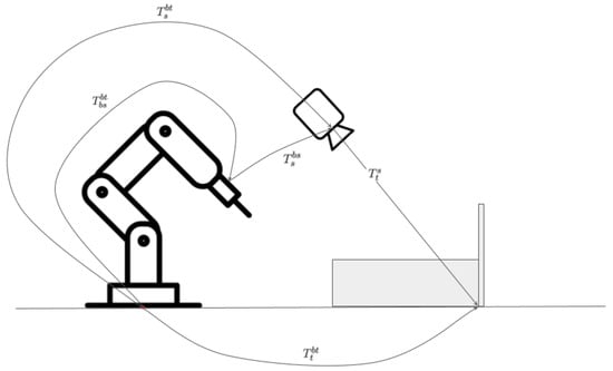
Figure 8.
Reference frames.
The camera mounted on the robot has its own base, which we refer to as the “base of the sensor” (bs).
The transformation matrix, denoted as T, plays a pivotal role in representing and manipulating objects in 3D space. It combines both rotation and translation information, providing a unified mathematical framework for describing changes in an object’s position and orientation.
Here, R is a 3 × 3 rotation matrix that describes how an object’s coordinate axes are rotated relative to a reference frame. The 3 × 1 translation vector t represents the object’s displacement, specifying how far it is shifted along each of the coordinate axes.
The robot’s internal system provides the first crucial transformation, denoted as , which maps the relationship between these two frames: the base of the target (bt) and the base of the sensor (bs). Essentially, this transformation tells us how the camera’s base is positioned and oriented relative to the robot’s base.
The second transformation accounts for the offset between the mounting point of the sensor (bs) and the sensor origin (s). This transformation is determined through hand-eye calibration using the Tsai procedure [22].
The homogeneous matrix in Equation (2) defines the position of the camera sensor with respect to the robot base frame:
The primary objective of this study was to determine , which is the transformation matrix that maps the weld point’s location relative to the robot’s base frame (bt). To achieve this, we needed to extract from the camera data, which represents the transformation matrix relating the weld point to the camera’s sensor frame (s).
We utilized the pinhole camera model [23,24] (Figure 9) to project the identified 2D pixel onto the 3D world.
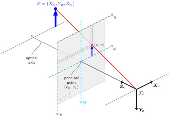
Figure 9.
Pinhole camera model.
To accurately project 3D points in the world coordinate frame onto the 2D image plane, we needed to consider both the camera’s internal parameters and its external position and orientation. The intrinsic camera matrix (K) captures the camera’s internal parameters (Equation (3)), such as the focal length and principal point, which are fixed for a given camera, and can be estimated using calibration procedures [25]. However, the camera’s position and orientation in the world coordinate frame are also crucial. This is where the extrinsic camera matrix (M) comes into play. The extrinsic matrix M combines both the camera’s rotation (R) and translation (t) relative to the world coordinate frame and can be expressed as a combination of the intrinsic camera matrix (K), rotation (R), and translation (t) according to M = K[R t] (Equation (6)). This matrix allows us to accurately project 3D world points to 2D image points, taking into account the camera’s pose and internal parameters.
For an undistorted image, the intrinsic calibration camera matrix K takes the form of Equation (3):
where and represent the focal lengths, and and represent the principal point offset, expressed in pixel units.
In the case where there are no rotation and no translation, M takes the form that can be seen in Equation (5):
We begin by determining . Using the pinhole camera model, a known 3D point in the camera frame can be projected onto the image plane using the perspective transformation K, resulting in the 2D pixel p in Equation (7):
where (u) and (v) are the coordinates of pixel p in the image plane, and , , and are the coordinates of point P in the camera frame.
Our goal was to find the 3D coordinates of the initial weld point based on the identified pixel p. We needed to establish reference frames to perform the calculations.
We know the transformation from Equation (2).
First, we express a point in camera coordinates to a point in the robot base frame using Equation (8):
Then, we multiply each side of the equation by the inverse of the transform , that is ; then, we obtain (9) and (10):
Using Equation (10) in Equation (7) and multiplying both sides by s allows us to calculate a point on the line passing through the camera center and the selected pixel according to Equation (11):
The scale factor s is introduced because a 2D pixel projected onto the 3D world could lie anywhere along the line connecting the camera center and the real 3D point. To calculate , we rearrange Equation (11) to give Equation (12):
Leveraging the pixel identified in Section 2.2.3, the robot transformation , and the camera matrix M, we can calculate two 3D points along the projection line by selecting two distinct values for the scale factor ‘s’. These points define a parametrized line equation representing the ray originating from the camera center and passing through the detected vertex in the image.
To ensure accurate 3D position estimation, we introduce a constraint by assuming the base plane (bt plane) is known. This is a valid assumption in our experimental setup, as the robot rests on the base piece, similar to the “Dandy” robot in a shipyard. If this plane is not readily available, it can be easily determined using a standard chessboard calibration technique [23,26].
With the known base plane, we can project the 2D pixel onto this plane, effectively finding the intersection point between the projection line (defined by the two 3D points) and the base plane. This intersection point represents the accurate 3D position of the initial weld point relative to the robot’s base frame.
3. Experiment Results and Discussion
3.1. Experimental Setup
To validate the effectiveness of the proposed initial weld point extraction method, a series of experiments were conducted. The experimental setup is illustrated in Figure 1. Two U-shaped samples were used in the experiments, one of which is shown in Figure 3. The experiments were conducted following a semi-straight line from approximately 0.5 to 1.5 m from the sensor to the target vertex, which are similar distances to those used in actual production. The experiments consisted of a series of captures of point clouds and images at the same position on the robot, with the aim of comparing the 2D and 3D errors.
3.2. Ground Truth Retrieval
With the aim to compare our novel method results with the 3D output, the vertex point was extracted from a point cloud obtained from the camera. Point Cloud Library (PCL), which is based on C++, was used to extract data from the point clouds. A pipeline was established to analyze the point cloud output of the camera, which was a disorganized collection of x, y, and z points. This pipeline was used to detect the vertices on the object. As the sensor moved away from the target, the scattered nature of the points in the point cloud necessitated a modified version of the pipeline, resulting in fewer points on the interesting planes. Figure 10 illustrates the general pipeline.

Figure 10.
Three-dimensional pixel extraction pipeline.
This section describes the extraction of vertex points from the 3D camera output to be compared with our novel method results. We leveraged the PCL to process the unorganized point cloud data (x, y, and z coordinates). A specialized pipeline extracted vertices from the point cloud.
Figure 10 illustrates the main steps:
- Downsampling: This reduces the density of the point cloud by grouping nearby points into 3D cubes (voxels), each with a side length of 2 mm. This process balances the accuracy and processing time by simplifying the point cloud while retaining relevant geometric information.
- RANSAC: The RANSAC (Random Sample Consensus) algorithm [27] was employed to extract planes from the point cloud. RANSAC works by iteratively selecting a minimal set of points (in this case, 500 points) to define a plane, and then evaluates the consensus of the remaining points against this plane. This process was repeated for a maximum of 100 iterations. A point was considered an inlier if its distance from the fitted plane was less than 3 mm. This robust approach effectively identified the dominant planes within the point cloud, even in the presence of noise and outliers.
- Plane intersection: Potential U-shaped structures were identified by verifying the near-perpendicularity of three extracted planes. To ensure a robust detection, we required that the planes formed angles close to 90 degrees, with a tolerance of 3 degrees. Additionally, we checked that each point within the point cloud was located within a maximum distance of 3 cm from the intersection points of all three planes. This combined approach effectively identified potential U-shaped structures by verifying both the geometric relationship between the planes and the spatial arrangement of the points within the point cloud.
- Vertex extraction: the intersection point of these three planes becomes the candidate vertex.
As the sensor’s distance from the target increases, the resulting point cloud becomes less dense, with fewer points representing the relevant planes. This sparsity poses a challenge for accurately identifying vertices. To address this, the pipeline incorporated several adaptive measures, requiring the manual adjustment of key parameters. The voxelization process, with a voxel size of 2 mm, was adjusted to account for the reduced point density, effectively clustering points into smaller 3D cubes to enhance the point cloud’s density. Furthermore, the RANSAC algorithm’s parameters, including the minimum number of points (500), maximum iterations (100), and distance threshold (3 mm), were manually adjusted to ensure robust plane extraction, even in scenarios with fewer points. The perpendicularity check, which verified the near-perpendicularity between planes with a tolerance of 3 degrees and a maximum point distance of 3 cm from the intersection points, was also adapted through manual adjustment to the changing point cloud density. This adaptive approach, which required manual parameter tuning, ensured efficient and reliable vertex extraction and provided a solid foundation for further analysis and comparison with our novel 2D image processing method.
We deemed a point to be a suitable choice for a vertex if it met the pre-defined criteria. We acquired a 3D point in the camera frame and then used the frames mentioned to transfer this point to the robot frame.
3.3. Two-Dimensional Feature Extraction Error
Section 2.2 explains how the novel method identifies points in an image as initial weld points. For each potential point, the method calculate the corresponding location on the image based on the known 3D ground truth position.
The “2D error” reflects the difference between the actual pixel location extracted from this method and the calculated pixel location from the 3D projection. This error is measured in pixels.
As can be seen in Figure 11, when the camera was close to the target, each pixel covered a smaller area, and thus, there were more pixels to choose from. Conversely, when the camera was farther away, each pixel encompassed a larger area, and thus, there were fewer pixels to choose from. In short, the closer to the camera, the less sensitive the method should be to pixel errors.
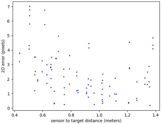
Figure 11.
Two-dimensional error distance in pixels.
3.4. Three-Dimensional Distance Error
Section 2.3 tackles the conversion of a 2D image to their corresponding locations on a 3D robot frame, using the target plane as the reference. In this comparison, a slight variation existed in the Z-coordinate of these points due to extrinsic calibration, which impacted their accurate matching.
To address this, we introduced the concept of a “3D error”. This metric measured the difference in meters between the actual 3D point from the point cloud and its calculated 2D counterpart derived from this novel method. The 3D location was calculated by elevating the reference plane at the Z-coordinate of the point cloud vertex.
By employing this approach, we could effectively compare points between the 3D point cloud and the 2D image, despite the Z-coordinate discrepancy caused by the calibration. This allowed for a more accurate assessment of the matching process and its potential limitations.
Figure 12 reveals a critical relationship between the sensor distance and distance error stability. Points within a 0.8–1.1 m range from the target exhibited the most consistent distance error values. This range presented a valuable balance, enabling the capture of the entire scene of interest in a single image while minimizing the impact of potential extrinsic calibration discrepancies associated with image fusion techniques requiring multiple sensor positions. Consequently, employing the sensor within this identified range facilitated the achievement of both comprehensive scene capture and accurate distance measurements within our experimental setup. This approach eliminates the need for image fusion, simplifying the measurement process and effectively mitigating potential extrinsic calibration errors. Further investigation into the influence of sensor resolution and environmental factors on distance error within this optimal range could provide valuable insights for future optimization efforts.
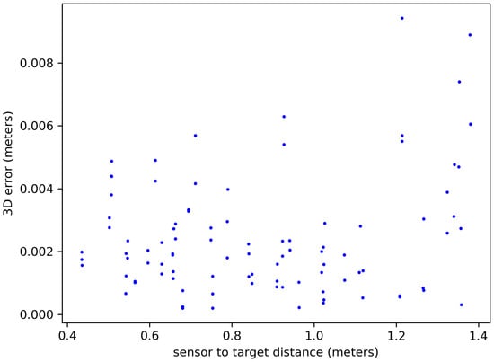
Figure 12.
Three-dimensional error distance in meters.
As detailed in Section 3.3, the sensor proximity to the target influenced the sensitivity of the pixel errors to real-world distances. With a closer sensor, each pixel represented a smaller area, reducing the impact of pixel-level discrepancies on resulting distance measurements. Conversely, at larger sensor distances, a single pixel covered a larger area, meaning the same pixel error translated to a bigger actual distance variation.
This effect can be seen when comparing Figure 11 and Figure 12. They highlight how the 3D error nearly quadrupled (from 0.4 to 1.4 m) for the same pixel error due to this distance-dependent sensitivity. Interestingly, the zone between 0.9 and 1.0 m appeared to offer a “sweet spot” with greater stability in the 3D error, despite the pixel variations.
This finding underscores the importance of considering the sensor distance when interpreting both 2D and 3D measurements. Selecting an appropriate distance range, such as the observed stable zone, can help to mitigate distance-related errors and improve the accuracy of the results.
3.5. Processing Time
This pipeline highlighted the contrasting processing times between point cloud and image analyses. While downsampling offered initial efficiency, the subsequent plane extraction, which is arguably the most complex step, scaled with the number of planes detected, leading to variable processing times. In contrast, pixel extraction in the 2D image analysis remained fairly consistent across images and primarily depended on the pixel count.
Table 2 reflects this disparity. On average, 3D point cloud processing required a significantly higher duration (6097 ms) compared with the 308 ms for image processing using CPU inference. Additionally, the standard deviation for the point cloud processing (3500 ms) underscored its greater variability compared with the image-processing deviation of 19 ms.

Table 2.
Image and point cloud processing times.
The optimal choice depends on the specific application’s requirements, balancing the need for detailed spatial data with the processing speed and cost constraints.
Compared with traditional point cloud approaches, this new method excelled in terms of speed, reducing the processing time by at least 50% and it was up to 50 times faster in complex scenarios. Figure 13 visually demonstrates the dramatic acceleration, especially for point clouds containing many planes. Further potential for performance gains lie in utilizing GPUs and optimizing debugging practices.
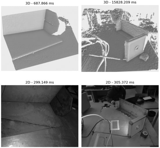
Figure 13.
Processing time comparison.
3.6. Lighting Conditions
The accuracy of the weld point extraction using vision systems can be significantly impacted by variations in lighting conditions and the angle of the sensor. Welding flares from other robots, especially in a multi-robot environment, pose a significant challenge for accurate image-based weld point identification.
To address these challenges, our research adopted a multi-pronged approach:
Controlled environment: Our initial experiments were conducted in a controlled laboratory environment to minimize the influence of external light sources. This allowed us to isolate the specific challenges related to our method before tackling the complexities of real-world scenarios.
Lighting variations: We conducted experiments using a curtain to create different illumination scenarios, simulating variations in lighting conditions. These experiments, illustrated in Figure 14, demonstrate that the point cloud data were more sensitive to lighting variations compared with the 2D images, highlighting the potential advantages of using 2D images for weld point extraction in challenging environments.
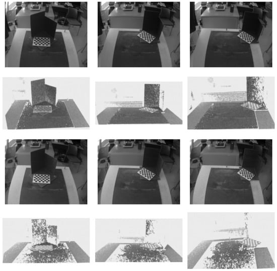
Figure 14.
Lighting variation comparison.
Sensor angle: We conducted experiments with the camera positioned at different angles relative to the workpiece, including 45 degrees, 90 degrees at 25 cm from the center, and 90 degrees at 40 cm from the center. These experiments, also illustrated in Figure 14, demonstrate that capturing both vertices in a single 2D image from a central position is possible in certain cases, whereas point clouds might require at least two captures, one for each vertex. This highlights the potential benefits of our 2D approach for capturing multiple weld points in a single image, potentially improving the efficiency and reducing the processing time.
Multi-robot scenarios: While completely eliminating welding flares might not be possible in multi-robot scenarios, we envision integrating our 2D pipeline with a synchronized control system for multiple robots. This synchronized system could potentially mitigate the impact of welding flares by considering the positions and movements of all robots within the workspace, ensuring that each robot’s vision system captures the weld points accurately.
Future research: We recognize the complexities of real-world welding environments and plan to investigate strategies for mitigating the impact of welding flares and other external light sources in future research. This could involve exploring methods for image pre-processing, such as noise reduction and adaptive thresholding, or developing more robust deep learning models that are less sensitive to lighting variations. We believe that our approach, by leveraging the advantages of 2D image processing, exploring the potential of single-image capture, and considering the potential for synchronized multi-robot systems, provides a promising foundation for addressing these challenges in future applications.
4. Conclusions
This paper presents a novel, cost-effective approach for initial weld point extraction using 2D RGB cameras and deep learning techniques. Our method leverages a two-stage YOLOv8s pipeline, combining object detection and semantic segmentation, to extract 3D keypoints from images. This approach offers significant cost advantages compared with traditional 3D point cloud methods, primarily due to the lower requirements for 2D camera lens accuracy.
Our approach demonstrates several key advantages:
- Cost-effectiveness: our method offers a significant cost reduction, up to 50 times lower compared with traditional RGB-D cameras, making it an attractive solution for industrial settings with budget constraints.
- Versatility: the use of 2D cameras provides flexibility and adaptability for various welding scenarios, as they are easier to integrate into existing robotic systems compared with more complex 3D sensing solutions.
- Robustness: our two-stage YOLO pipeline was found to be effective in identifying keypoints, particularly in scenarios with low-contrast images, such as those produced by grayscale cameras and dark metal surfaces.
- Efficiency: Initial tests, which were conducted in simulation using an ROS and structured robot data, demonstrated near real-time performance. Further optimization with GPU acceleration and reduced data saving can potentially enhance the speed and efficiency.
While 3D point cloud approaches offer greater accuracy in certain scenarios, our 2D image-based approach demonstrates its potential for versatility and cost-efficiency. The 3D pipeline, relying primarily on analytical plane extraction, exhibits slower performance for high-resolution or complex point clouds. Our 2D approach, while requiring training and retraining for different objects and scenarios, offers a promising alternative for applications where cost and flexibility are paramount.
Key findings:
- We developed a methodology for identifying keypoints from 3D point clouds.
- We present a novel 2D image-based approach for detecting 3D keypoints, incorporating robot positioning information.
- We conducted a comparative analysis that demonstrated the potential benefits and limitations of both 2D and 3D approaches.
This advancement holds significant potential for real-world industrial applications, where efficient and reliable weld point extraction is critical for automated welding processes.
Author Contributions
Conceptualization, M.-A.L.-F., A.M.-E., I.D.-C. and F.J.B.; data curation, M.-A.L.-F. and I.D.-C.; formal analysis, M.-A.L.-F. and F.J.B.; funding acquisition, A.M.-E. and F.J.B.; investigation, M.-A.L.-F., A.M.-E., I.D.-C. and F.J.B.; methodology, M.-A.L.-F. and F.J.B.; project administration, A.M.-E. and F.J.B.; resources, A.M.-E. and F.J.B.; software, M.-A.L.-F. and I.D.-C.; supervision, A.M.-E. and F.J.B.; validation, M.-A.L.-F. and I.D.-C.; visualization, A.M.-E. and F.J.B.; writing—original draft, M.-A.L.-F. and I.D.-C.; writing—review and editing, M.-A.L.-F., A.M.-E. and F.J.B. All authors read and agreed to the published version of this manuscript.
Funding
This work was partially support by the Programme for Attracting Talent of University of Cadiz, and was developed in the framework of the AUROVI Project, supported by the Ministry of Science, Innovation and Universities under grant EQC2018-005190-P.
Data Availability Statement
The data that support the findings of this study are available from the corresponding author upon request.
Acknowledgments
M.-A.L.-F. acknowledges support from the University of Cadiz (UCA) and Instrumentación y control del sur S.L (SURCONTROL) for his predoctoral positions.
Conflicts of Interest
The authors declare no conflicts of interest.
Abbreviations
The following abbreviations are used in this manuscript:
| ROS | Robot operating system |
| SAM | Segment Anything Model |
| YOLO | You Only Look Once |
| PCL | Point Cloud Library |
| POI | Point of interest |
| CUDA | Compute unified device architecture |
| SGD | Stochastic gradient descent |
References
- Mandal, N.R. Ship Construction and Welding; Springer: Berlin/Heidelberg, Germany, 2017; Volume 2. [Google Scholar] [CrossRef]
- Lee, D.; Ku, N.; Kim, T.W.; Kim, J.; Lee, K.Y.; Son, Y.S. Development and application of an intelligent welding robot system for shipbuilding. Robot. Comput. Integr. Manuf. 2011, 27, 377–388. [Google Scholar] [CrossRef]
- Dinham, M.; Fang, G. Detection of fillet weld joints using an adaptive line growing algorithm for robotic arc welding. Robot. Comput. Integr. Manuf. 2014, 30, 229–243. [Google Scholar] [CrossRef]
- Zhang, L.; Xu, Y.; Du, S.; Zhao, W.; Hou, Z.; Chen, S. Point Cloud Based Three-Dimensional Reconstruction and Identification of Initial Welding Position. In Transactions on Intelligent Welding Manufacturing; Springer: Singapore, 2018; pp. 61–77. [Google Scholar] [CrossRef]
- Gao, J.; Li, F.; Zhang, C.; He, W.; He, J.; Chen, X. A Method of D-Type Weld Seam Extraction Based on Point Clouds. IEEE Access 2021, 9, 65401–65410. [Google Scholar] [CrossRef]
- Kim, J.; Lee, J.; Chung, M.; Shin, Y.G. Multiple weld seam extraction from RGB-depth images for automatic robotic welding via point cloud registration. Multimed. Tools Appl. 2020, 80, 9703–9719. [Google Scholar] [CrossRef]
- Yang, S.; Shi, X.; Tian, X.; Liu, Y. An Approach to the Extraction of Intersecting Pipes Weld Seam Based on 3D Point Cloud. In Proceedings of the 2022 IEEE 11th Data Driven Control and Learning Systems Conference (DDCLS), Chengdu, China, 3–5 August 2022. [Google Scholar]
- Patil, V.; Patil, I.; Kalaichelvi, V.; Karthikeyan, R. Extraction of Weld Seam in 3D Point Clouds for Real Time Welding Using 5 DOF Robotic Arm. In Proceedings of the 2019 5th International Conference on Control, Automation and Robotics (ICCAR), Beijing, China, 19–22 April 2019. [Google Scholar]
- Wei, S.c.; Wang, J.; Lin, T.; Chen, S.b. Application of image morphology in detecting and extracting the initial welding position. J. Shanghai Jiaotong Univ. Sci. 2012, 17, 323–326. [Google Scholar] [CrossRef]
- Liu, F.; Wang, Z.; Ji, Y. Precise initial weld position identification of a fillet weld seam using laser vision technology. Int. J. Adv. Manuf. Technol. 2018, 99, 2059–2068. [Google Scholar] [CrossRef]
- Yang, L.; Fan, J.; Liu, Y.; Li, E.; Peng, J.; Liang, Z. Automatic Detection and Location of Weld Beads With Deep Convolutional Neural Networks. IEEE Trans. Instrum. Meas. 2021, 70, 5001912. [Google Scholar] [CrossRef]
- Li, J.; Liu, Z.; Wang, J.; Gu, Z.; Shi, Y. A novel initial weld position identification method for large complex components based on improved YOLOv5. In Proceedings of the 2023 3rd International Conference on Robotics and Control Engineering, Nanjin, China, 12–14 May 2023. [Google Scholar]
- Stanford Artificial Intelligence Laboratory. Robotic Operating System. Available online: https://www.ros.org/ (accessed on 24 June 2024).
- Rusu, R.B.; Cousins, S. 3D is here: Point Cloud Library (PCL). In Proceedings of the IEEE International Conference on Robotics and Automation (ICRA), Shanghai, China, 9–13 May 2011. [Google Scholar]
- Jocher, G.; Chaurasia, A.; Qiu, J. YOLO, Version 8; Ultralytics: Los Angeles, CA, USA, 2023.
- Ku, N.; Ha, S.; Roh, M.I. Design of controller for mobile robot in welding process of shipbuilding engineering. J. Comput. Des. Eng. 2014, 1, 243–255. [Google Scholar] [CrossRef][Green Version]
- Shinichi, S.; Muraoka, R.; Obinata, T.; Shigeru, E.; Horita, T.; Omata, K. Steel Products for Shipbuilding; JFE Technical Report; JFE Holdings: Tokyo, Japan, 2004. [Google Scholar]
- Hussain, M. YOLO-v1 to YOLO-v8, the Rise of YOLO and Its Complementary Nature toward Digital Manufacturing and Industrial Defect Detection. Machines 2023, 11, 677. [Google Scholar] [CrossRef]
- Detect—Ultralytics YOLOv8 Docs. Available online: https://docs.ultralytics.com/tasks/detect/ (accessed on 24 June 2024).
- Dwyer, B.; Nelson, J.; Solawetz, J. Roboflow, Version 1.0; Roboflow: Des Moines, IA, USA, 2022.
- Kirillov, A.; Mintun, E.; Ravi, N.; Mao, H.; Rolland, C.; Gustafson, L.; Xiao, T.; Whitehead, S.; Berg, A.C.; Lo, W.Y.; et al. Segment Anything. In Proceedings of the IEEE/CVF International Conference on Computer Vision (ICCV), Paris, France, 2–6 October 2023. [Google Scholar]
- Tsai, R.Y.; Lenz, R.K. A New Technique for Fully Autonomous and Efficient 3D Robotics Hand/Eye Calibration. IEEE Trans. Robot. Autom. 1989, 5, 345–358. [Google Scholar] [CrossRef]
- OpenCV: Camera Calibration and 3D Reconstruction. Available online: https://docs.opencv.org/3.4/d9/d0c/group__calib3d.html (accessed on 24 June 2024).
- Hartley, R.; Zisserman, A. Multiple View Geometry in Computer Vision; Cambridge University Press: Cambridge, UK, 2004. [Google Scholar] [CrossRef]
- Dawson-Howe, K.M.; Vernon, D. Simple pinhole camera calibration. Int. J. Imaging Syst. Technol. 1994, 5, 1–6. [Google Scholar] [CrossRef]
- Ha, J.E. Automatic detection of chessboard and its applications. Opt. Eng. 2009, 48, 067205. [Google Scholar] [CrossRef]
- Fischler, M.A.; Bolles, R.C. Random sample consensus. Commun. ACM 1981, 24, 381–395. [Google Scholar] [CrossRef]
Disclaimer/Publisher’s Note: The statements, opinions and data contained in all publications are solely those of the individual author(s) and contributor(s) and not of MDPI and/or the editor(s). MDPI and/or the editor(s) disclaim responsibility for any injury to people or property resulting from any ideas, methods, instructions or products referred to in the content. |
© 2024 by the authors. Licensee MDPI, Basel, Switzerland. This article is an open access article distributed under the terms and conditions of the Creative Commons Attribution (CC BY) license (https://creativecommons.org/licenses/by/4.0/).