Defining the Consistent Velocity of Omnidirectional Mobile Platforms

Abstract

The maximum linear (or translational) velocity achievable by an omnidirectional platform is not uniform as it depends on the angular orientation of the motion. This velocity is limited by the maximum angular velocity of the motors driving the wheels and also depends on the mechanical configuration and orientation of the wheels. This paper proposes a procedure to compute an upper bound for the translational velocity, named the consistent velocity of the omnidirectional platform, which is defined as the minimum of the maximum translational velocities achievable by the platform in any angular orientation with no wheel slippage. The consistent velocity is then a uniform translational velocity always achievable by the omnidirectional platform regardless of the angular orientation of the motion. This paper reports the consistent velocity for a set of omnidirectional platforms with three omni wheels that have the same radius and angular distribution but different angular orientations. Results have shown that these platforms can achieve different maximum velocities in different angular orientations although the consistent velocity is the same for all of them. Results have also shown that the consistent velocity has a linear relation with the angular velocity of the motion. The consistent velocity of a mobile platform can be used by its path-planning algorithm as an upper bound that guarantees the execution of any omnidirectional motion at a uniform and maximum translational velocity.

1. Introduction

Omnidirectional platforms are defined by their ability to combine translation and rotation in any direction due to the absence of constraints in their kinematics. Because of their excellent mobility performance, omnidirectional robots are being introduced in a wide range of sectors such as logistics [1], material conveying in manufacturing plants [2], inspection in harsh environments [3], search and rescue in disaster situations [4], elderly assistance [5], and services such as cleaning [6]. However, in general, in mobile robotic applications, the use of holonomic platforms is less common than differential drive systems [7], which are mechanically simpler and easier to maintain.

In the scientific literature, there are a significant number of works presenting and analyzing different types of omnidirectional mobile platforms. However, the analysis of the maximum allowable translational velocity of a mobile platform is not usually addressed during motion analysis and trajectory planning. Some application examples that would benefit from the analysis of the maximum allowable translational velocity of the mobile platform are listed below. Tian et al. [8] presented the motion features analysis of platforms with six and four omnidirectional wheels. Terakawa et al. [9] studied the motion characteristics of a mecanum-wheeled robot on a slope to determine the effect of wheel skidding on the maximum acceleration and the straight-traveling stability according to the angle of the slope. Galati et al. [10] designed a robot for industrial applications and modeled its kinematic and dynamic behaviors to tackle slippage and vibrations affecting the accuracy of pose estimation and tracking control. Mohanraj et al. [11] assessed the importance of the fourth wheel in a four-wheeled robot with omni wheels. Thai et al. [12] presented a trajectory-tracking controller for mobile robots with mecanum wheels by time-varying the parameters of the PID controller. Li et al. [13] proposed topological design methods to judge omnidirectionality for mobile robots with mecanum-wheeled configurations, although their procedure can be generally applied to any type of omnidirectional wheels with passive rollers. Almasri et al. [14] developed a mathematical model that optimizes motion performances of omnidirectional platforms using symmetrical wheel distributions.

The maximum translational (or linear) velocity achievable by an omnidirectional platform is not uniform as it depends on the angular orientation of the motion and the parameters of the platform [15]. The limitations caused by the maximum translational velocity of a mobile platform have been addressed by Balkcom et al. [16] and Kim et al. [17] in the computation of minimum-time trajectories. In their proposals, the common objective was to take advantage of the angular orientations providing the maximum translational velocities of the platforms. Balkcom et al. [16] analyzed the fastest trajectories of a mobile robot with three omni wheels, obtaining time-optimal trajectories that contained only spins in place, circular arcs, and straight lines parallel to wheel axles. Kim et al. [17] addressed the computation of the minimum-time trajectory by imposing that at least one motor must have the maximum angular velocity, presenting a systematic procedure to construct an optimal control input vector.

The understanding of the upper bound velocity limit that represents the consistent velocity for an omnidirectional mobile platform will allow for the development of new research focused on the computation of maximum-uniform-velocity trajectories. This feature can be especially useful when omnidirectional platforms must operate in spaces shared with people because maintaining a uniform velocity will make their trajectory more predictable for people moving around.

1.1. New Contribution

The new contribution of this work is a procedure to compute the consistent velocity of an omnidirectional platform. The consistent velocity is an upper bound of the translational velocity, defined as the minimum of the maximum translational velocities achievable by an omnidirectional platform when moving in any angular orientation with no wheel slippage. The consistent velocity is then a uniform translational velocity always achievable by the omnidirectional platform regardless of the angular orientation of the motion. The upper bound defined by the consistent velocity guarantees the execution of any omnidirectional motion at a uniform and maximum translational velocity.

This paper reports the computation of the consistent velocity for a set of platform configurations with three omni wheels, which is the minimum number of omni wheels required to achieve omnidirectional mobility [13]. The consistent velocity can be used by the path-planning algorithm of the platform to maximize its velocity while guaranteeing the execution of the motions planned. Finally, since the consistent velocity defines a limitation, this parameter can also be used to maximize motion capabilities during the design stage of a new omnidirectional platform configuration.

1.2. Structure of the Paper

The paper is structured as follows. Section 2 describes the materials and methods used. Section 3 presents the problem caused by the maximum velocities of the motors. Section 4 defines the consistent velocity and describes the procedure used to compute it. Section 5 presents the results obtained for a set of omnidirectional mobile platforms. Section 6 discusses the results obtained. Finally, Section 7 provides the conclusions of the paper and possible future works.

2. Materials and Methods

The materials used in this paper are a set of example platform configurations that are analyzed to obtain their maximum translational velocities and their consistent velocity. The method used is the kinematic model of omnidirectional platforms.

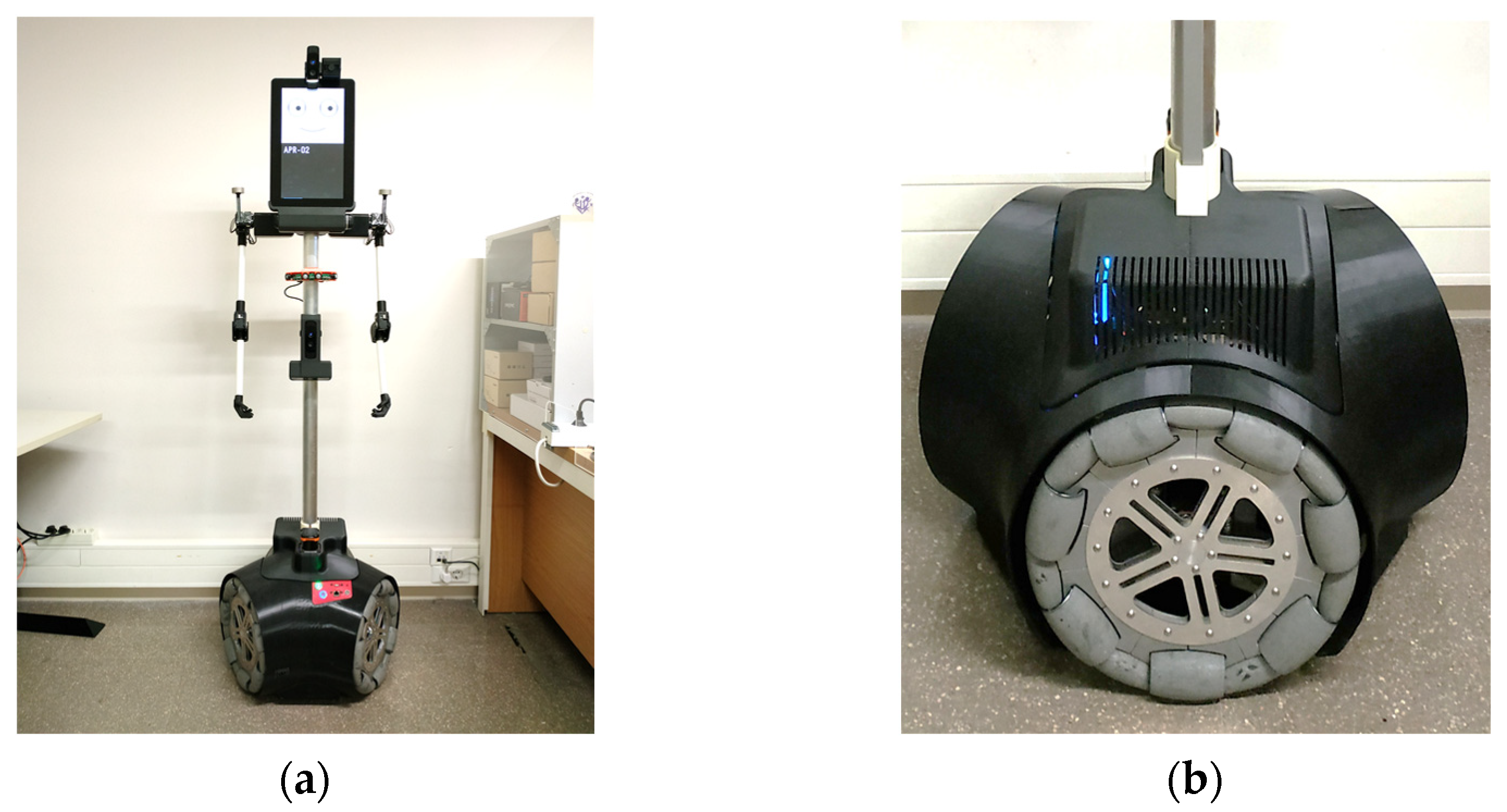
2.1. Platform Configurations Assessed

Figure 1a presents the definition of the dimensional parameters of the set of three-wheeled omnidirectional mobile platforms that are assessed in this work. This parametric definition is proposed to simplify the interpretation of the mechanical configuration of the platforms. Figure 1a defines the world frame $\left\{s\right\}$, which is static; the platform frame $\left\{b\right\}$, which is attached to the body of the platform; and the wheel frame $\left\{w_k\right\}$, which is specific to each wheel. A number $k$ is assigned to identify each wheel. The $x_b$ axis in the platform frame defines the forward direction of the system, and in each wheel frame, the ${y_{\mathrm{w}}}_k$ axis is aligned with the wheel hub.

Table 1. Mobile platform configurations assessed in this work: name, schematic representation, and angular orientation of the wheels (${\phi }_k$).

Name	3A	1A-2B	1A-2C	1A-1B-1C	1A-1B-1D	3E
Diagram
${\mathit{\phi }}_{\mathit{k}=\mathbf{1}\dots \mathbf{3}}$(°)	[0 0 0]	[−90 0 −90]	[30 0 −30]	[0 −90 −30]	[0 −90 60]	[49.37 49.37 49.37]

summarizes the parametric information of the platforms analyzed. Table 1 proposes an identifying name, a schematic top-view representation of the configurations, and the angular orientation of their wheels (${\phi }_k$) according to the parametric definition presented in Figure 1. All the platform configurations assessed have three omnidirectional wheels with rollers at ${\gamma }_k=0°$(Figure 1b), which are named omni wheels (Mecanum wheels have ${\gamma }_k=45°$, Figure 1c). All the wheels of the platforms assessed have the same radius ($r_{k=1\dots 3}=0.148 \mathrm{m}$), the same distance to the centroid of the platform ($R_{k=1\dots 3}=0.195 \mathrm{m}$), and the same angular distribution (${\delta }_{k=1\dots 3}=\left[60 180 300\right]°$). Therefore, the differences between the mobile platforms assessed are only their wheel orientations (${\phi }_k$).

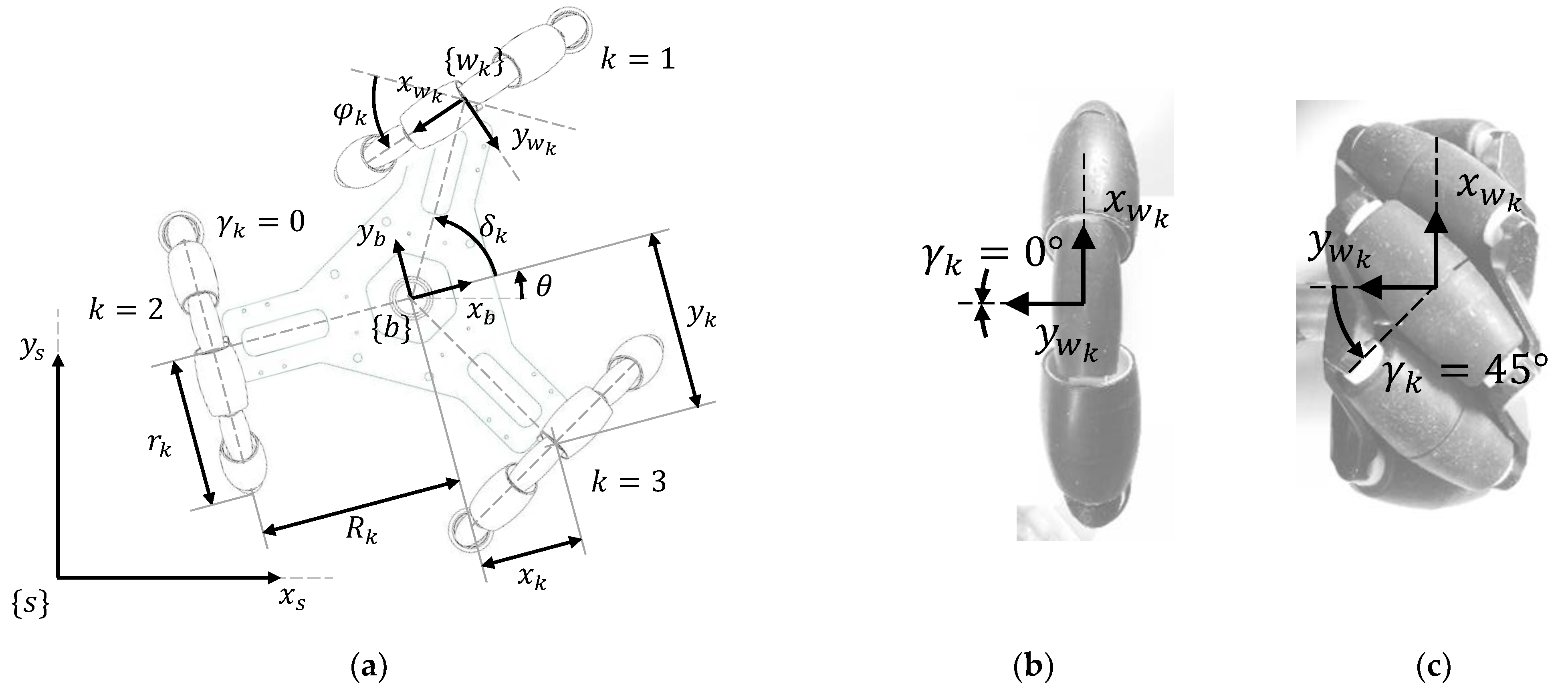
2.2. Kinematic Model of an Omnidirectional Platform

The motion of an omnidirectional platform can be controlled with a motion command defined in the platform frame $M={\left(v,\alpha ,\omega \right)}_{\left\{b\right\}}$, where $v_{\left\{b\right\}}$ is the norm of the translational velocity of the platform, ${\alpha }_{\left\{b\right\}}$ is the angular orientation of the translational velocity of the platform (angular orientation of the motion), and ${\omega }_{\left\{b\right\}}$ is the angular velocity of the platform. The specific advantage of an omnidirectional platform is that it can move in any angular orientation $\alpha$ (in a full range from 0° to 360°) while simultaneously rotating at an angular velocity $\omega$. The combination of different translational and angular velocities results in linear and curved trajectories with different radii and orientations.

The motion command $M$ is provided by the path-planning algorithm implemented in the central control unit of the mobile platform while the path-tracking algorithm computes the kinematics of the platform to obtain the angular velocities of the wheels ${\omega }_k$ required to implement the planned path. The total linear velocity of one wheel $k$ has two components, one in the drive direction (${\overrightarrow{v}}_{k,drive}$, collinear with the wheel plane) and one in the slide direction (${\overrightarrow{v}}_{k,slide}$, parallel with the free-rolling direction):

$${\overrightarrow{v}}_{k,total}={\overrightarrow{v}}_{k,drive}+{\overrightarrow{v}}_{k,slide}.$$

(1)

The drive direction is coincident with the wheel plane; its velocity makes the wheel advance forward or backward because it is the result of the angular velocity of the wheel:

$$v_{k,drive}=r_k·{\omega }_k.$$

(2)

The slide direction is coincident with the free-rolling direction of the passive rollers in the omni wheel; its velocity makes the wheel slide laterally in the direction of the wheel hub.

The general procedure to obtain the kinematic model is, for each wheel [18], to (1) define the motion command $M={\left(v,\alpha ,\omega \right)}_{\left\{b\right\}}$ and then express the velocities in the platform frame as ($v_x$,$v_y$,$\omega$); (2) transform these velocities to the wheel frame; (3) decompose the linear velocity of the wheel in the drive (wheel) and slide (roller) directions; and (4) assume that there is no slip to compute the target angular velocity of the wheel ${\omega }_k$ to be transferred to the board controlling the rotation of the motors attached to the wheels. The resulting equation that defines the angular velocity of any wheel $k$ of the platform is as follows:

$${\omega }_k=\left[\begin{array}{cc}\frac{1}{r_k}& \frac{\tan \left({\gamma }_k\right)}{r_k}\end{array}\right]·A_{b\to {\mathrm{w}}_k \left(R\right)}·A_{b\to {\mathrm{w}}_k \left(T\right)}·{\left[\begin{array}{c}{v}_x\\ v_y\\ \omega \end{array}\right]}_{\left\{b\right\}},$$

(3)

where $A_{b\to {\mathrm{w}}_k \left(T\right)}$ and $A_{b\to {\mathrm{w}}_k \left(R\right)}$ are the translation and rotation matrixes, respectively, required to express the motion command in the wheel frame:

$$A_{b\to {\mathrm{w}}_k \left(T\right)} =\left[\begin{array}{ccc}1& 0& -y_k\\ 0& 1& x_k\end{array}\right],$$

(4)

$$A_{b\to {\mathrm{w}}_k \left(R\right)}=\left[\begin{array}{cc}\cos \left({ϵ}_k\right)& \sin \left({ϵ}_k\right)\\ -\sin \left({ϵ}_k\right)& \cos \left({ϵ}_k\right)\end{array}\right].$$

(5)

The rotation angle${ϵ}_k$ is defined as ${ϵ}_k={\phi }_k+{\delta }_k+90°$ (see Figure 1).

The extended expression obtained from Equation (3) in the case of working with omni wheels (whose angle of the passive rollers is ${\gamma }_k=0°$) results in the following:

$${\omega }_k=\left[\begin{array}{ccc}\frac{\cos \left({ϵ}_k\right)}{r_k}& \frac{\sin \left({ϵ}_k\right)}{r_k}& \frac{x_k\sin \left({ϵ}_k\right)-y_k\cos \left({ϵ}_k\right)}{r_k}\end{array}\right]·{\left[\begin{array}{c}{v}_x\\ v_y\\ \omega \end{array}\right]}_{\left\{b\right\}}.$$

(6)

The general inverse kinematic model of a motion system used to compute the velocities of a three-wheeled omnidirectional platform (for $k=1\dots 3$) is computed using the following:

$$\left[\begin{array}{c}{\omega }_1\\ {\omega }_2\\ {\omega }_3\end{array}\right]=J\left[\begin{array}{c}{v}_x\\ v_y\\ \omega \end{array}\right],$$

(7)

with $J$ being the following matrix:

$$J=\left[\begin{array}{c}\begin{array}{ccc}\frac{\cos \left({ϵ}_1\right)}{r_1}& \frac{\sin \left({ϵ}_1\right)}{r_1}& \frac{x_1\sin \left({ϵ}_1\right)-y_1\cos \left({ϵ}_1\right)}{r_1}\end{array}\\ \begin{array}{ccc}\frac{\cos \left({ϵ}_2\right)}{r_2}& \frac{\sin \left({ϵ}_2\right)}{r_2}& \frac{x_2\sin \left({ϵ}_2\right)-y_2\cos \left({ϵ}_2\right)}{r_2}\end{array}\\ \begin{array}{ccc}\frac{\cos \left({ϵ}_3\right)}{r_3}& \frac{\sin \left({ϵ}_3\right)}{r_3}& \frac{x_3\sin \left({ϵ}_3\right)-y_3\cos \left({ϵ}_3\right)}{r_3}\end{array}\end{array}\right].$$

(8)

This matrix depends on the radii ($r_k$) of the omni wheels, the angular orientation (${\phi }_k$) of the wheels, the angular distribution (${\delta }_k$) of the wheels, the angular orientation of the rollers (${\gamma }_k$) of the wheels (which in this case is ${\gamma }_k=0°$), and the distance between the centroids of the platform and the wheels in the directions of the axes of the platform frame ($x_k, y_k$). Finally, the expression that defines the forward kinematics of the platform is as follows:

$$\left[\begin{array}{c}{v}_x\\ v_y\\ \omega \end{array}\right]=J^{-1}\left[\begin{array}{c}{\omega }_1\\ {\omega }_2\\ {\omega }_3\end{array}\right].$$

(9)

This last expression is the one used by the central control unit of the mobile platform to estimate the odometry of the motion from the information provided by the encoders attached to the wheels or the motors of the platform [19,20].

3. Problem Definition

3.1. Maximum Translational Velocity of a Mobile Platform

The maximum translational velocity of an omnidirectional mobile platform with omni wheels depends on the mechanical configuration (radius, placement, and orientation) of the wheels and on the maximum angular velocity allowed by the motors driving the wheels. As stated in the introduction, the limitation imposed by the motors of the platform is rarely considered when planning the motion; the assumption is that the maximum angular velocity of the motors is never reached. However, if the target angular velocities of the wheels exceed the limit imposed by the maximum angular velocity of the motors, then the platform performs a trajectory that is different from the expected one.

This paper addresses the problem of computing an upper bound for the translational velocity of an omnidirectional mobile platform with three omni wheels. The path-planning algorithm controlling the mobile platform can use this upper bound to avoid the generation of motion commands that require exceeding the maximum velocity allowed by the motors driving the wheels of the platform. The application of this upper bound limit guarantees the correct execution of the planned motions.

3.2. Problem Caused by the Maximum Velocity of the Motors

This section is proposed to describe and highlight the problem caused in an omnidirectional platform in case of defining motions exceeding the limit imposed by the maximum angular velocity allowed by the motors driving its wheels. This effect is described and analyzed in a practical case with the APR robot [21]. Figure 2a shows the entire mobile robot and Figure 2b details one of its three omni wheels implementing the 3A configuration (defined in Table 1). This mobile robot has been applied to develop different mobile robotic applications [22,23,24], registering, in some cases, small trajectory inaccuracies of unknown origin attributed to various possible causes. This robot has a symmetric configuration, with the same distance between the centroid of the robot and each wheel ($R_k$), the same wheel radius ($r_k$), and 120° wheel distribution (${\delta }_{k=1\dots 3}=\left[60,180,300\right]°$).

Figure 2b shows the omni wheels used by the robot, which are based on free rollers that can slide perpendicularly to the wheel plane (${\gamma }_k=0°$). The rollers provide the wheel with velocity in the slide direction, while the rotation of the wheel results in a linear velocity in the drive direction. The addition of both velocity components defines the velocity and motion of the robot. In this example case [21], the maximum velocity allowed by the motors driving the wheels of the platform is ${\omega }_{max}=6.70$ rad/s, so any target wheel velocity above this limit cannot be reached.

The effect that the maximum angular velocity of the motors can have on the mobility of a system is represented in Figure 3, which shows the trajectory of the robot implementing a motion command $M$ with and without considering the limiting effect imposed by the maximum angular velocity reachable by its motors. Figure 3 shows the theoretically expected robot trajectory (cyan, solid line), which does not consider the limiting effect of the maximum angular velocity of the motors driving the wheels, and the ground truth trajectory of the robot (red, dashed line) registered by its onboard odometry (affected by the limit imposed by the maximum angular velocity of the motors). In both cases, the initial position $p_i$ is defined in the world origin ($x=0 \mathrm{m},y=0 \mathrm{m}, \theta =0°$) with the robot facing forwards, and the target motion command applied during two seconds to the robot to control its motion is $M=\left[1 \mathrm{m}/\mathrm{s}, 0°, 1 \mathrm{rad}/\mathrm{s}\right]$.

Theoretically, the target angular velocities (${\omega }_k$) of the three omni wheels to reach the final position $p_f=\left[0.92 \mathrm{m}, 1.41 \mathrm{m}, 114.8°\right]$ are ${\omega }_1=-4.53$ rad/s ($-43.25 \mathrm{rpm}$), ${\omega }_2=1.32$ rad/s ($12.60 \mathrm{rpm}$), and ${\omega }_3=7.17$ rad/s ($68.46 \mathrm{rpm}$). However, the maximum angular velocity of the motors is $6.7$ rad/s, so wheel 3 surpasses this value and, in practice, the angular velocity of the wheels is saturated to ${\omega }_{k=\mathrm{1...3},TRUTH}=\left[-4.53, 1.32, 6.70\right]$ rad/s. As a result, the robot follows a different trajectory (Figure 3, red, dashed line) and reaches a different final position $p_{f,TRUTH}=\left[1.10 \mathrm{m}, 1.26 \mathrm{m}, 101.2°\right]$. The practical result is that the robot performs a trajectory that is different from the expected one, and the cause of this anomalous trajectory is difficult to identify during practical application.

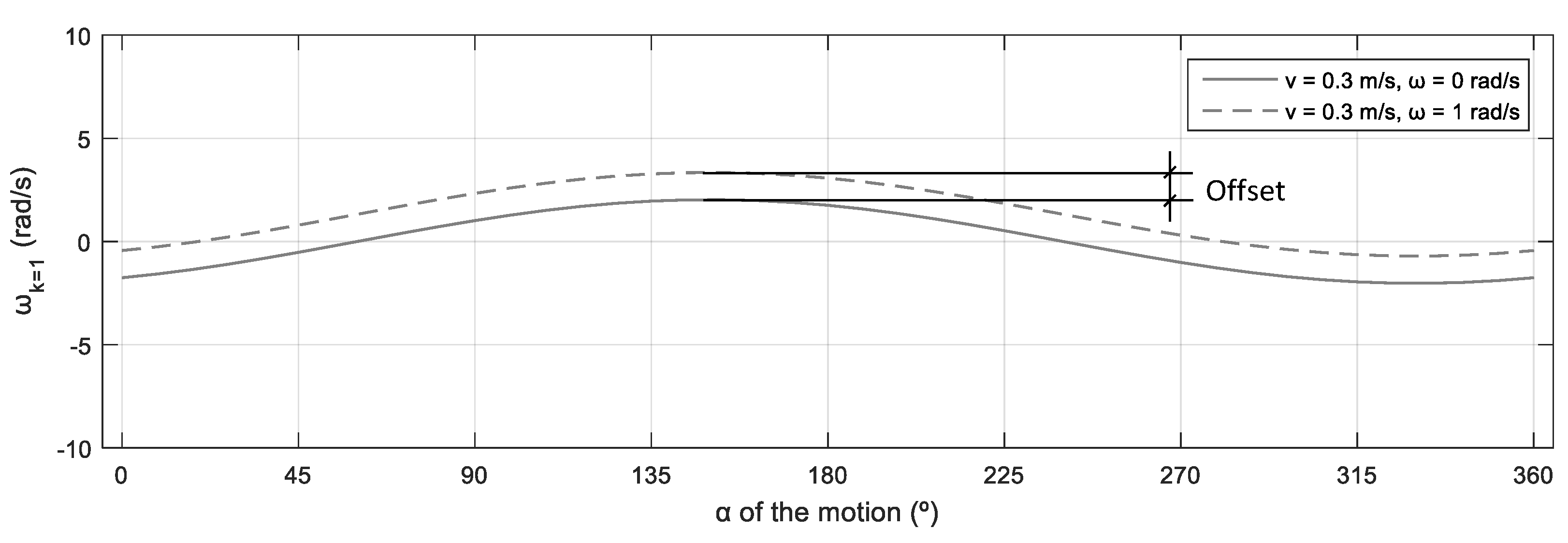
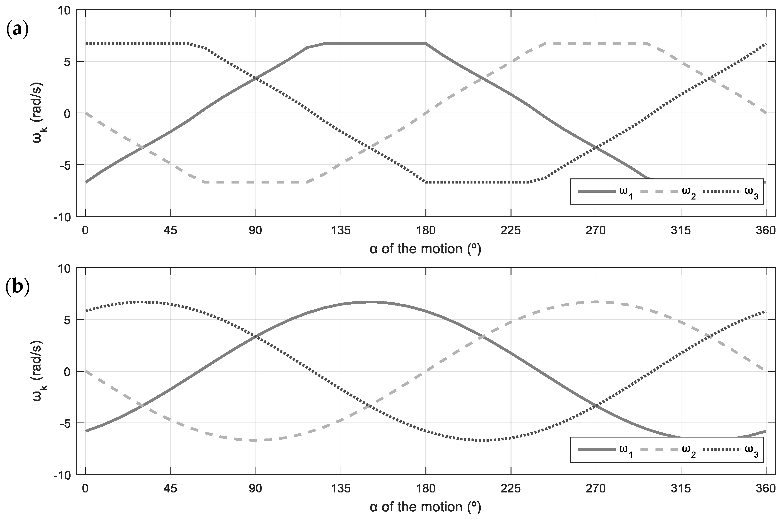
3.3. Profile of the Angular Velocities of the Wheels

For the sake of completeness, this section represents the profile of the angular velocities of the omni wheels relative to the angular orientation of the motion in a 3A mobile platform. The sinusoidal profile that defines this relationship is common to any omnidirectional platform configuration and must be understood to properly interpret the procedure proposed to compute the consistent velocity.

Given a motion command $M={\left(v,\alpha ,\omega \right)}_{\left\{b\right\}}$, Figure 4 shows the evolution of the angular velocity of wheel 1 (${\omega }_{k=1}$) of the 3A mobile platform [21,25] represented as a function of the angular orientation $\alpha$ of the motion. This profile is computed with the inverse kinematics equation of the mobile platform (Equation (7)). The solid line represents the profile for $v=0.3$ m/s and $\omega =0$ rad/s and the dashed line represents the profile for $v=0.3$ m/s and $\omega =1$ rad/s. The difference between the two profiles relays only on the different angular velocities applied to the mobile platform.

Figure 4 shows that the representation of the profiles of ${\omega }_{k=1}$ relative to the angular orientation $\alpha$ of the linear velocity has a characteristic sinusoidal shape. The difference in the angular velocity of the platform $\omega$ generates a vertical offset in the sinusoidal profile, which has the same value for the whole range of angular orientations $\alpha$. Interestingly, the offset is not dependent on the linear velocity of the platform $v$, but on its angular velocity $\omega$. This offsetting effect caused by the angular velocity $\omega$ must be taken into consideration when defining an upper bound for the translational velocity.

4. Consistent Velocity

4.1. Consistent Velocity Definition

The term consistent velocity is sometimes used as a synonym for constant velocity. The term is occasionally used in hydrodynamic calculations [26] and in the construction field to evaluate the bearing capacity for foundations on unsaturated soils [27]. In this paper, we propose the term consistent velocity ($vcons$) to define an intrinsic parameter of omnidirectional platforms. In this context, the consistent velocity is defined as the minimum of the maximum translational velocities achievable by an omnidirectional platform in any direction.

As a summary, the consistent velocity defines an upper velocity bound that can be used to guarantee the execution of the planned motion commands without setting unreachable angular velocities to the motors driving the wheels (see Figure 3). Basically, this can be conducted by verifying if the norm of the translational velocity defined in any motion command satisfies the velocity limits defined by the consistent velocity $v\in \left[0,vcons\right]$.

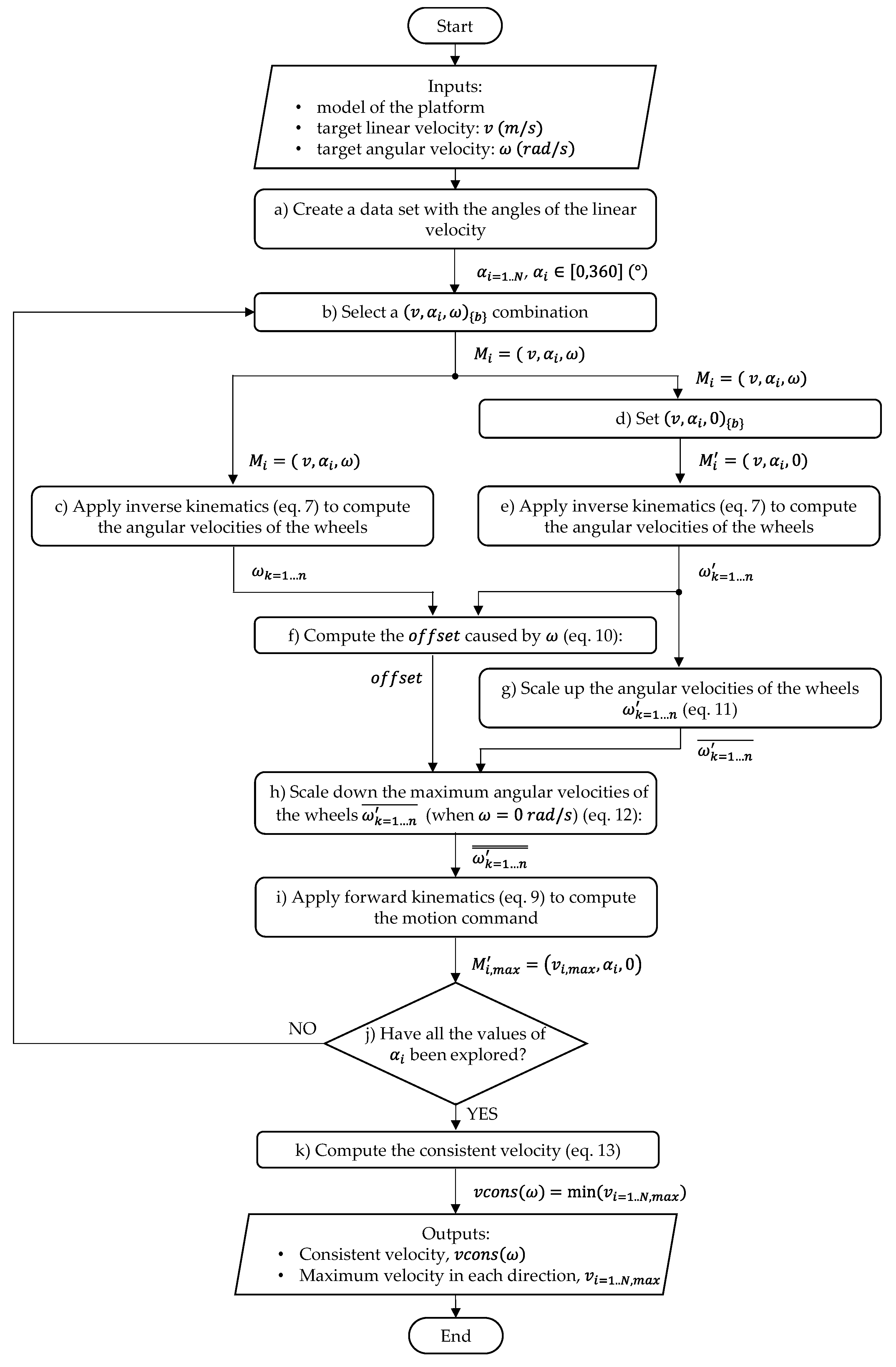
4.2. Consistent Velocity Computation

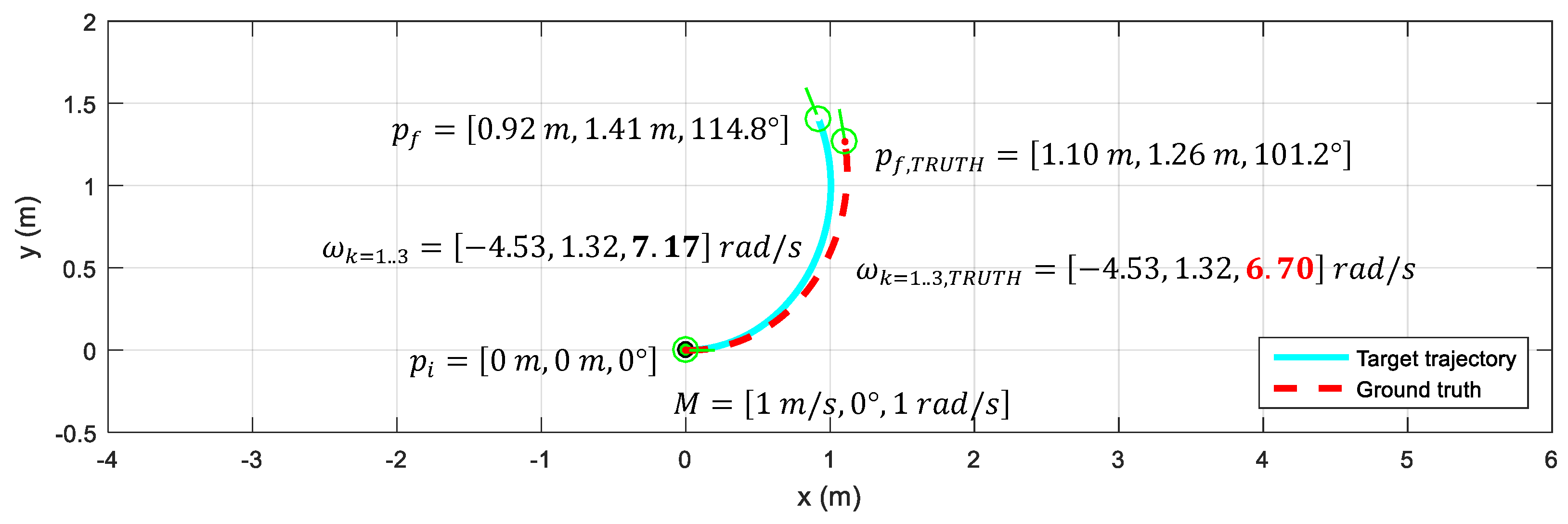
The computation of the consistent velocity of an omnidirectional platform is based on the determination of the maximum translational velocity of the platform in each angular orientation of the motion. The computation procedure is based on the analysis of a set of motion commands defined with the same norm of the linear velocity of the platform $v$, the same angular velocity of the platform $\omega$, and a set of angular orientations of the linear velocity (${\alpha }_{i=1\dots N}$) covering all the angular orientations of the motion. To this end, the procedure computes the maximum linear velocity of the platform $v_{i,max}$ in each motion direction ${\alpha }_i$. To do so, each motion command $M_i={\left(v,{\alpha }_i,\omega \right)}_{\left\{b\right\}}$ defined in the platform frame is analyzed to obtain the maximum reachable translational velocity $v_{i,max}$, defining an upper bound for the motion command $M_{i,max}={\left(v_{i,max},{\alpha }_i,\omega \right)}_{\left\{b\right\}}$. Hence, the only difference between $M_i$ and $M_{i,max}$ is the substitution of the linear velocity $v$ with the maximum reachable value $v_{i,max}$ that is later analyzed to obtain the consistent velocity from the minimum value of $v_{i=1\dots N,max}$. In order to perform this computation, an auxiliary motion command $M_i^{\prime }={\left(v,{\alpha }_i,0\right)}_{\left\{b\right\}}$ is defined with the same values as the motion command $M_i$, but with the angular velocity being $\omega =0$ rad/s.

Figure 5 shows the flowchart describing the procedure defined to obtain the consistent velocity of an omnidirectional platform. The inputs of the process are the model of the platform (see Figure 1 and Table 1), the norm of a target linear velocity of the platform ($v$), and a target angular velocity of the platform ($\omega$). The norm of the linear velocity $v$ is used as a seed value that is later normalized, so its initial value is not relevant. The outputs are the consistent velocity of the platform ($vcons$) and the maximum velocity ($v_{i,max}$) reachable in each angular orientation of the motion. The procedure is as follows.

The first step a) creates the data set with the angles of the linear velocity ${\alpha }_{i=1\dots N}$ to be explored, where $N$ defines the number of elements of the dataset, and ${\alpha }_i$ ranges from 0° to 360°.

The second step b) is the selection of one angular orientation from the data set to create a motion command $M_i=\left(v,{\alpha }_i,\omega \right)$, which is later used in the computations of step c) and step d).

Step c) computes the angular velocities of the wheels ${\omega }_{k=1\dots n}$ required to execute the motion command $M_i=\left(v,{\alpha }_i,\omega \right)$ by the mobile platform. These angular velocities are computed using Equation (7). Step d) sets the auxiliary motion command without the angular velocity of the platform $M_i^{\prime }=\left(v,{\alpha }_i,0\right)$, and step e) computes the angular velocities of the wheels $\omega {\prime }_{k=1\dots n}$ required to execute this auxiliary motion command. These angular velocities are used later in the computations of step f) and step g).

Then, step f) computes the maximum difference between the angular velocities of the wheels ${\omega }_{k=1\dots n}$ and $\omega {\prime }_{k=1\dots n}$. The result of this step is the $offset$ caused by $\omega$, where:

$$\left|offset\right|=\max \left(\left|{\omega }_{k=1\dots n}-{{\omega }^{\prime }}_{k=1\dots n}\right|\right),$$

(10)

and the sign of the $offset$ is maintained from the original difference ${\omega }_{k=1\dots n}-{{\omega }^{\prime }}_{k=1\dots n}$.

Next, in step g), the angular velocities of the wheels $\omega {\prime }_{k=1\dots n}$ (computed in step d) for $\omega =0$) are scaled up so that they reach the maximum angular velocity (${\omega }_{max}$) allowed by the motors driving the wheels:

$$\overline{{\omega }_{k=1\dots n}^{\prime }}=\frac{{\omega }_{max}·\omega {\prime }_{k=1\dots n}}{\max \left(\left|{{\omega }^{\prime }}_{k=1\dots n}\right|\right)}.$$

(11)

In step h), the scaled angular velocities of the wheels $\overline{{\omega }_{k=1\dots n}^{\prime }}$ are scaled down according to the value of the $offset$ required to execute the target angular velocity $\omega$ of the motion command $M_i=\left(v,{\alpha }_i,\omega \right)$:

$$\stackrel{=}{{\omega }_{k=1\dots n}^{\prime }}=\overline{{\omega }_{k=1\dots n}^{\prime }}·\frac{{\omega }_{max}-\left|offset\right|}{{\omega }_{max}}.$$

(12)

Next, in step i), the forward kinematics (Equation (9)) is applied to $\stackrel{=}{{\omega }_{k=1\dots n}^{\prime }}$ to compute the motion command $M_{i,max}^{\prime }=\left(v_{i,max},{\alpha }_i,0\right)$ required to obtain these angular velocities in the wheels of the platform.

Given that the calculation of $\stackrel{=}{{\omega }_{k=1\dots n}^{\prime }}$ is performed under the restrictions imposed by the offset that causes the angular velocity of the platform $\omega$, the maximum linear velocity in the motion command $M_{i,max}^{\prime }=\left(v_{i,max},{\alpha }_i,0\right)$ is the one that has to be applied to the platform to allow its rotation. Hence, the motion command $M_{i,max}=\left(v_{i,max},{\alpha }_i,\omega \right)$ defines the maximum translational velocity of the mobile platform $v_{i,max}$ in the angular orientation ${\alpha }_i$ when the angular velocity of the robot is $\omega$.

Step j) checks if all the directions ${\alpha }_{i=1\dots N}$ have been explored. If not, the process returns to step b). When all the angular orientations have been explored, the maximum translational velocity of the mobile platform $v_{i,max}$ in each angular orientation ${\alpha }_i$ is known and the consistent velocity can be computed.

Finally, step k) computes the consistent velocity $vcons$ of the mobile platform as the minimum value of the maximum linear velocities obtained when the angular velocity of the robot is $\omega$:

$$vcons\left(\omega \right)=\min \left(v_{i=1\dots N,max}\right) \mathrm{for} M_{i=1\dots N,max}=\left(v_{i=1\dots N,max},{\alpha }_i,\omega \right).$$

(13)

When the angular velocity of the platform is set to $\omega =0$ rad/s, there is no $offset$, and the scaled-up angular velocities of the wheels computed in step g) ($\overline{{\omega }_{k=1\dots n}^{\prime }}$) are the maximum ones in that configuration. In such case, the computation of the consistent velocity is computed as follows:

$$vcons=vcons\left(0\right)=\min \left(v_{i=1\dots N,max}\right) \mathrm{for} M_{i=1\dots N,max}^{\prime }=\left(v_{i=1\dots N,max},{\alpha }_i,0\right).$$

(14)

A MATLAB script performing all the steps needed to compute the consistent velocity is provided in [28]. Although this procedure has many steps, its computation requires only a few seconds in an average personal computer, since there are no minimization searches or iterative adjustments involved. Finally, this work aims to assess the consistent velocity of alternative omnidirectional platforms with three omni wheels, but its parametric formulation allows its direct application to more complex platforms, with additional or redundant omni wheels, just by using the appropriate kinematics describing the platforms.

5. Results

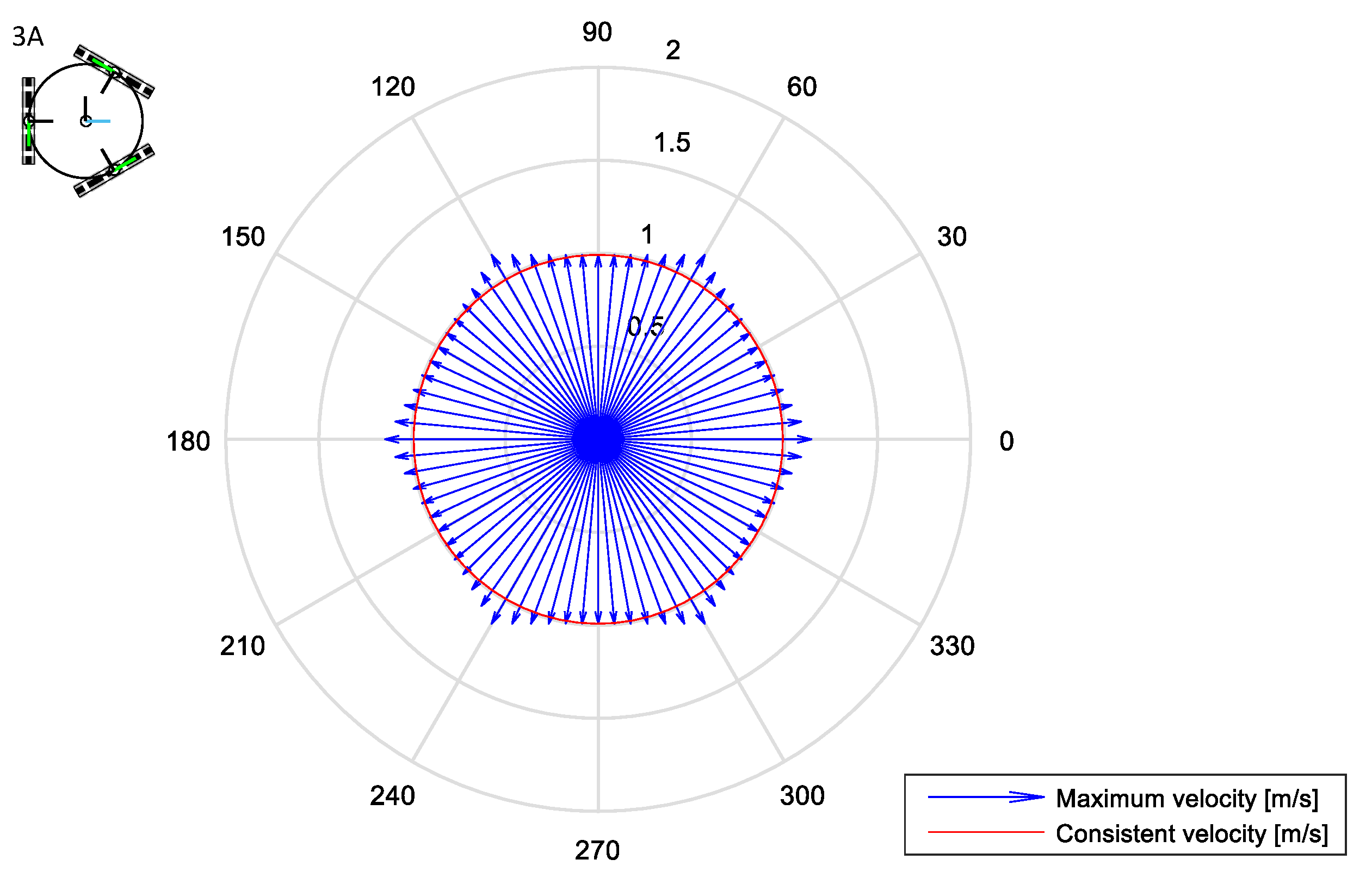
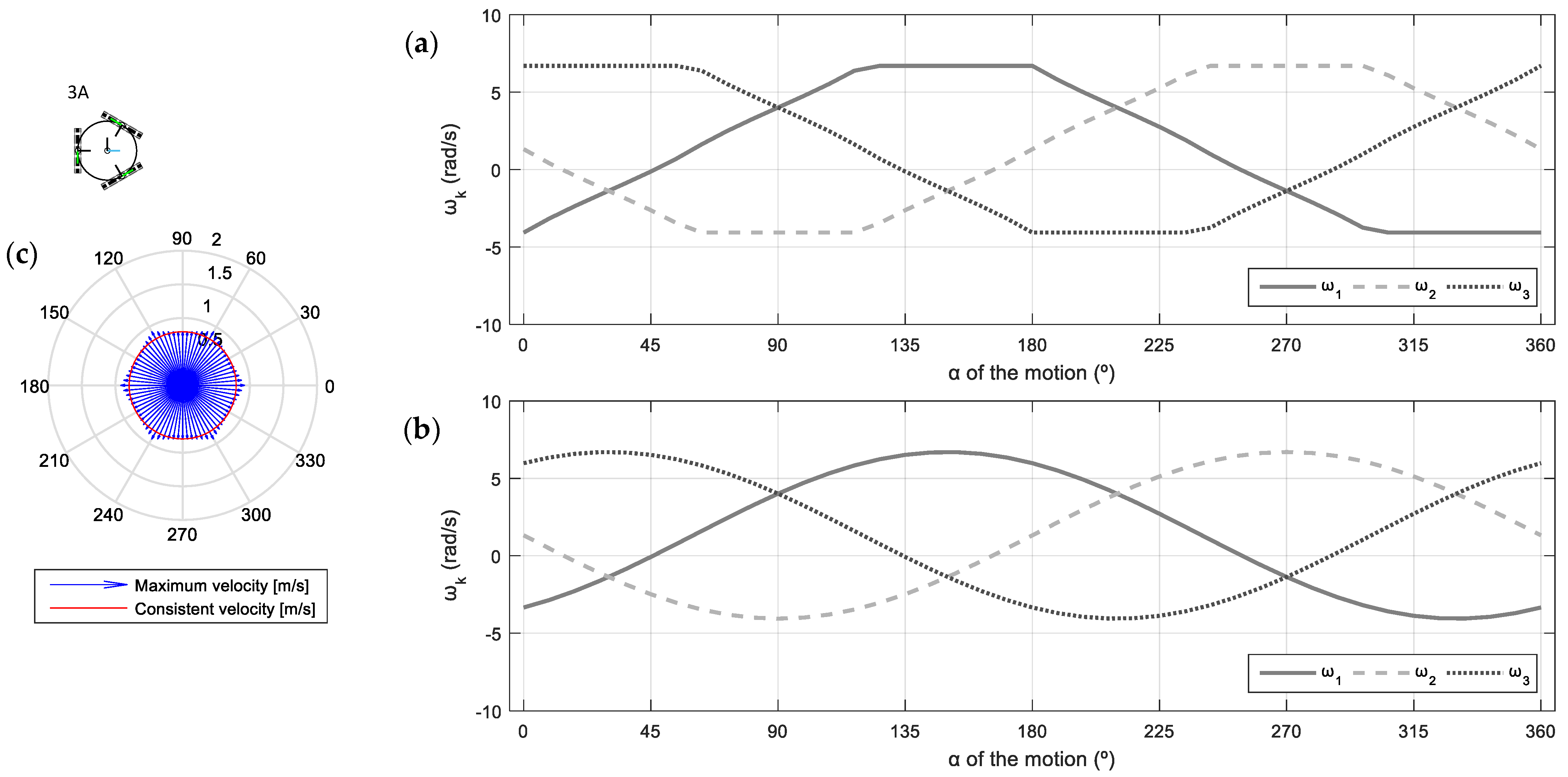
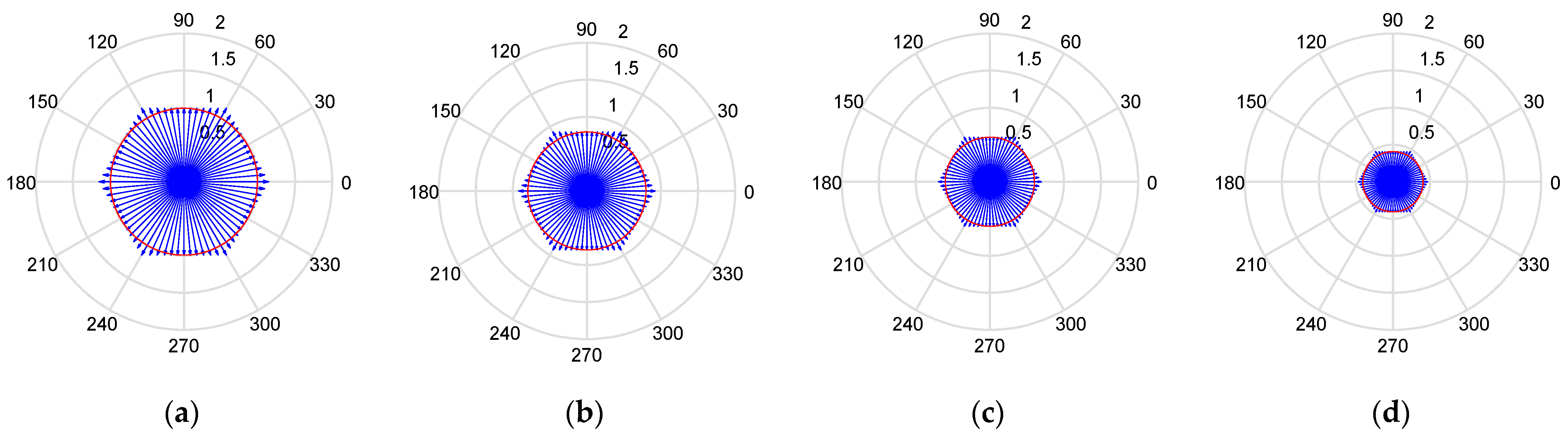
5.1. Consistent Velocity of the 3A Platform

This section presents the computation of the maximum translational velocities and the consistent velocity of the 3A omnidirectional platform (see Table 1) given different values of the angular velocity of the platform $\omega$.

5.1.1. Mobile Platform 3A: Consistent Velocity for $\omega =0 \mathrm{rad}/\mathrm{s}$

Figure 6 shows the maximum translational velocities and the consistent velocity of the 3A omnidirectional platform when the angular velocity of the platform is $\omega =0 \mathrm{rad}/\mathrm{s}$. The maximum translational (or linear) velocities are represented as blue arrows in a polar chart to simplify their interpretation. The center of the chart is the center of the mobile platform analyzed, which faces forward towards the 0° direction. The length of the blue arrows depicts the norm of the maximum translational velocities $v_{i=1\dots N,max}$ that can be achieved in the directions defined by the angular orientations ${\alpha }_{i=1\dots N}$ of the motion.

The polar chart in Figure 6 shows that the maximum translational velocities have an evolution that defines a characteristic hexagonal shape, where the maximum translational velocities are achieved at angular orientations coincident with the angular distribution of the wheels (60°, 180°, and 300°) and their mirrored angles (0°, 120°, and 240°). Complementarily, the minimum values of the translational velocities are achieved at orientations 30°, 90°, 150°, 210°, 270°, and 330°, just halfway between the angular orientations defined by the absolute maximums. When $\omega =0 \mathrm{rad}/\mathrm{s}$, the maximum translational velocities of the 3A platform are between 0.99 m/s and 1.15 m/s, while its consistent velocity (minimum of the maximum translational velocities) is 0.99 m/s, which is represented with a red circle in the polar chart.

Figure 7 represents the angular velocities of the wheels that correspond to the linear velocities shown in Figure 6, for the case $\omega =0 \mathrm{rad}/\mathrm{s}$. Figure 7a shows the profile of the angular velocities of the wheels that define the maximum translational velocities achieved by the platform as a function of the angular orientation of the motion $\alpha$. This profile is saturated because, in each angular orientation, one of the wheels must rotate at its maximum velocity. Alternatively, Figure 7b shows the non-saturated profile of the angular velocities of the wheels obtained when the translational velocity is the consistent velocity.

5.1.2. Mobile Platform 3A: Consistent Velocity for $\omega =1 \mathrm{rad}/\mathrm{s}$

This section computes the maximum translational velocities and the consistent velocity of the 3A omnidirectional platform when the angular velocity of the platform is $\omega =1 \mathrm{rad}/\mathrm{s}$.

The polar chart in Figure 8c shows that the maximum linear velocities maintain the characteristic hexagonal shape obtained in the previous case for $\omega =0 \mathrm{rad}/\mathrm{s}$, but with a smaller diameter because the maximum linear velocities are lower to allow the rotation at $\omega =1 \mathrm{rad}/\mathrm{s}$. The maximum of the maximum velocities is achieved at the same angular orientations as the case with $\omega =0 \mathrm{rad}/\mathrm{s}$ (0°, 60°, 120°, 180°, 240°, and 300°), just as the minimum values (30°, 90°, 150°, 210°, 270°, and 330°). When $\omega =1 \mathrm{rad}/\mathrm{s}$, the maximum velocities of the 3A platform are between 0.80 m/s and 0.92 m/s, while its consistent velocity (minimum of the maximum translational velocities) is 0.80 m/s, represented with a red circle.

Similarly to the previous section, Figure 8a shows the profile of the angular velocities of the wheels that define the maximum translational velocities achieved by the platform depending on the angular orientation of the motion $\alpha$. This profile is again saturated because, in each angular orientation, one of the wheels must rotate at its maximum velocity while allowing a rotation of the platform at $\omega =1 \mathrm{rad}/\mathrm{s}$. Alternatively, Figure 8b shows the non-saturated profile of the angular velocities of the wheels obtained when the translational velocity is limited according to the upper bound imposed by the consistent velocity.

Table 2. Comparison of the parameters of the velocity profiles of the 3A mobile platform.

Parameter	Case with $\mathit{\omega } = 0 \mathbf{rad}/\mathbf{s}$	Case with $\mathit{\omega } = 1 \mathbf{rad}/\mathbf{s}$	Case with $\mathit{\omega } = -1 \mathbf{rad}/\mathbf{s}$
Consistent velocity	0.99 m/s	0.80 m/s	0.80 m/s
Maximum of the maximum translational velocities	1.15 m/s	0.92 m/s	0.92 m/s
Minimum of the maximum translational velocities	0.99 m/s	0.80 m/s	0.80 m/s
$offset$ value	0 rad/s	1.32 rad/s	−1.32 rad/s
Maximum velocity of the wheels (${\omega }_1,{\omega }_2,{\omega }_3)$	6.70 rad/s	6.70 rad/s	4.07 rad/s
Minimum velocity of the wheels (${\omega }_1,{\omega }_2,{\omega }_3)$	−6.70 rad/s	−4.07 rad/s	−6.70 rad/s

compares the values of the most important parameters of the velocity profiles obtained in the previous section for $\omega =0 \mathrm{rad}/\mathrm{s}$ (Figure 7), with the ones from this section for $\omega =1 \mathrm{rad}/\mathrm{s}$ (Figure 8), and the parameters obtained for $\omega =-1 \mathrm{rad}/\mathrm{s}$. The consistent velocity computed for $\left|\omega \right|=1 \mathrm{rad}/\mathrm{s}$ is lower than for the case $\omega =0 \mathrm{rad}/\mathrm{s}$. The maximum and minimum velocities of the wheels displayed in Table 2 show the effect of the $offset$ in the angular velocities of the wheels, originated by the angular velocity of the platform $\omega$ (see Figure 4).

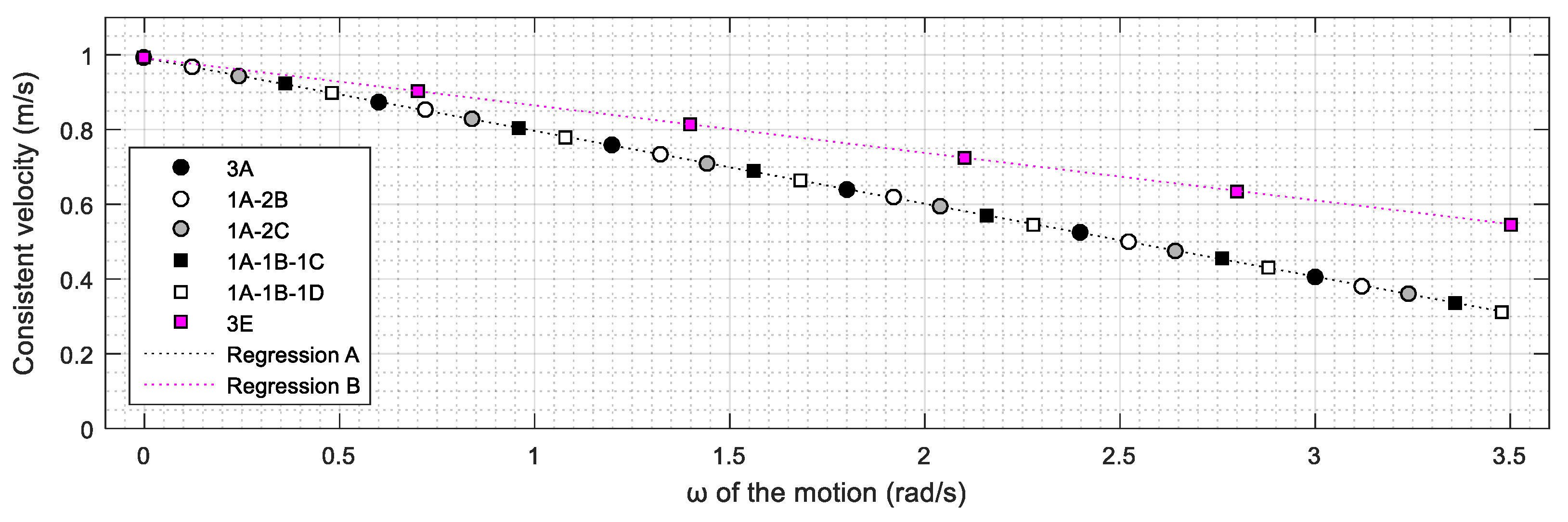
5.1.3. Mobile Platform 3A: Consistent Velocity as a Function of $\omega$

This section highlights the relationship between the angular velocity ($\omega$) and the consistent velocity of the 3A mobile platform. Figure 9 presents four polar charts showing the consistent velocity (red circle) and the maximum linear velocity $v_{i,max}$ (blue arrows) that can be achieved in each angular orientation ${\alpha }_i$ of the motion. The polar charts represent the following cases: (a) $\omega =0 \mathrm{rad}/\mathrm{s}$; (b) $\omega =1 \mathrm{rad}/\mathrm{s}$; (c) $\omega =2 \mathrm{rad}/\mathrm{s}$; and (d) $\omega =3 \mathrm{rad}/\mathrm{s}$. Although not shown, the polar charts obtained for a specific value of $\omega$ are the same when the angular velocity is positive and negative. The maximum linear velocity and the consistent velocity decrease as the angular velocity of the platform increases.

The linear relationship between the consistent velocity and the angular velocity of any mobile platform is analyzed later in Section 5.2.2.

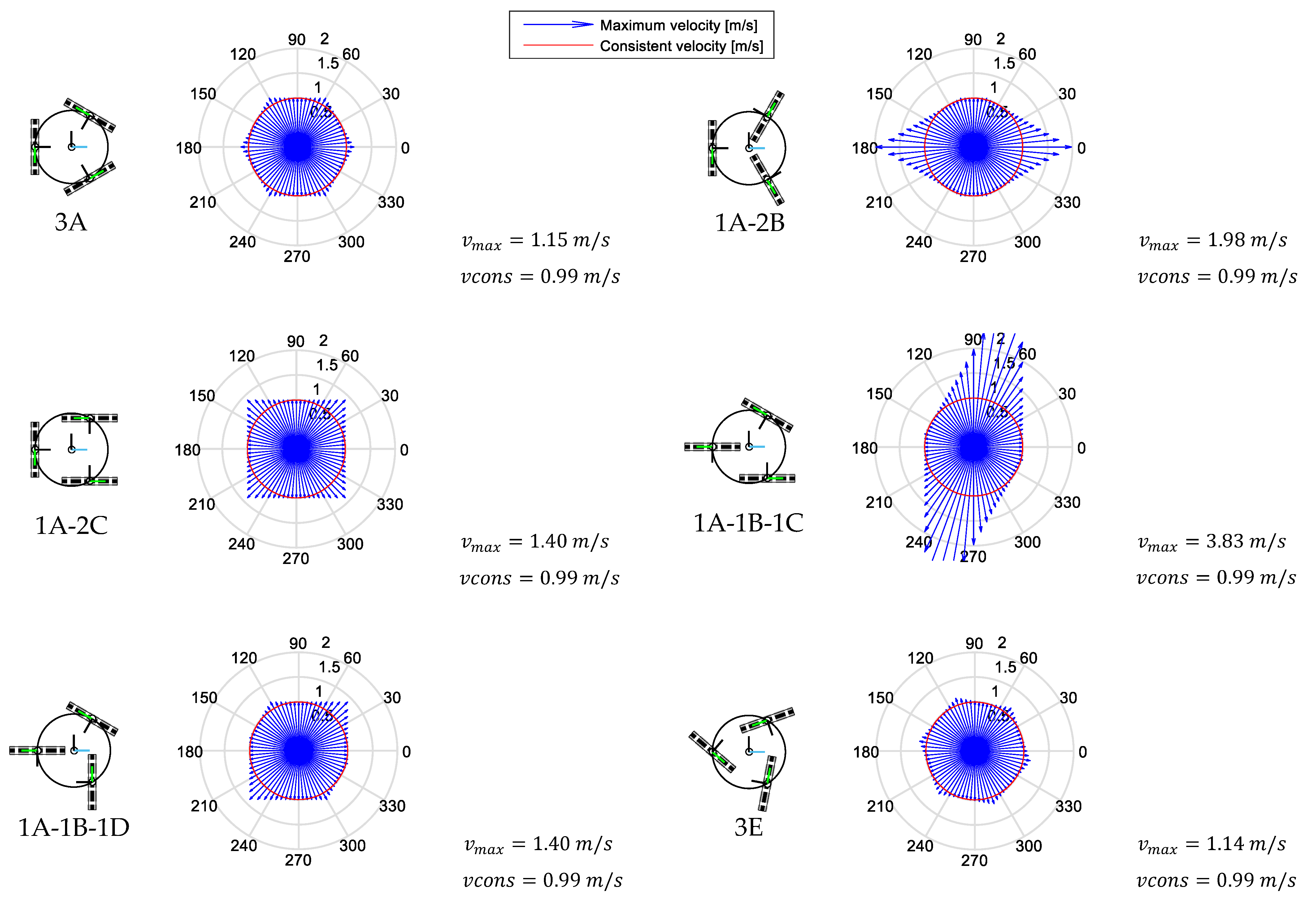
5.2. Consistent Velocity of the Set of Mobile Platforms

5.2.1. Consistent Velocity for $\omega =0 \mathrm{rad}/\mathrm{s}$

This section presents the consistent velocities and the maximum velocities of the set of omnidirectional platforms defined in Table 1 for the case with an angular velocity of the platform of $\omega =0 \mathrm{rad}/\mathrm{s}$.

Figure 10 depicts a schematic representation of each of the mobile platforms analyzed, their name, the polar chart representing the maximum velocity achieved in each angular orientation (blue arrows) and the consistent velocity (red circle). Figure 10 also details the maximum value of the maximum velocities achieved by the mobile platform $v_{max}$ and the value of the consistent velocity $vcons$ obtained for $\omega =0 \mathrm{rad}/\mathrm{s}$.

At this point, it is interesting to remember that all mobile platforms assessed in this paper have the same omni wheels with the same radius, placed at the same distance from the centroid of the mobile platform and with the same angular distribution (${\delta }_{k=1\dots 3}=\left[60 180 300\right]°$). Therefore, the only difference between the mobile platforms assessed is the orientation of their wheels (${\phi }_k$, see Table 1).

The shapes defined by the maximum translational velocities (blue arrows) of each mobile platform are certainly different. The 3A omnidirectional mobile platform, which is the most used, shows a typical hexagonal profile, with the maximum value of the maximum velocities being 1.15 m/s and the consistent velocity being 0.99 m/s. Interestingly, the 1A-2B platform has an elongated hexagonal shape that depicts two symmetric directions in which the platform can move faster (at 1.98 m/s) than 3A (at 1.15 m/s) despite having the same consistent velocity. In this case, this higher maximum velocity is because of the free rotation of the rollers, which makes the linear velocity of the wheels acquire a component in the slide direction, forcing the platform to move faster. The 1A-2C platform shows a square shape with the maximum of the maximum velocities being 1.40 m/s and a consistent velocity of 0.99 m/s. The 1A-1B-1C platform shows a shifted rhomboid shape which, in theory, allows the platform to move up to 3.83 m/s in the angular orientations ${\alpha }_i=75°$ and ${\alpha }_i=255°$, although difficult controllability may be expected during the motion of this platform. Despite these differences, the consistent velocity of the 1A-1B-1C configuration is also 0.99 m/s. The 1A-1B-1D platform shows a deformed hexagonal shape with the maximum of the maximum velocities being 1.40 m/s and the consistent velocity being 0.99 m/s. Finally, the 3E platform shows a hexagonal shape shifted 49.37° with respect to 3A, with a maximum velocity of 1.14 m/s and a consistent velocity of 0.99 m/s. Therefore, the consistent velocity of all the platforms assessed is as follows:

$$vcons=0.99 \mathrm{m}/\mathrm{s},$$

(15)

a value that is analyzed in the discussion section.

5.2.2. Consistent Velocity for $\omega \ne 0 \mathrm{rad}/\mathrm{s}$

This section analyses the evolution of the consistent velocity of the mobile platforms assessed for the cases of $\omega \ne 0 \mathrm{rad}/\mathrm{s}$. To this end, Figure 11 represents the values of the consistent velocity of the different mobile platforms assessed for a range of angular velocities from 0 rad/s (no rotation) to 3.5 rad/s (approximately half revolution in 1 s). As argued in the previous section, all the platforms have the same consistent velocity for the case $\omega =0 \mathrm{rad}/\mathrm{s}$, so other similarities can be expected in the relationship between the consistent velocity and the angular velocity $\omega$ of the motion. Figure 11 shows that the evolution of the consistent velocity relative to the angular velocity $\omega$ of the motion is the same for the platforms 3A, 1A-2B, 1A-2C, 1A-1B-1C, and 1A-1B-1D and can be expressed as the following (Figure 11-regression A):

$$vcons\left(\omega \right)=0.9916-0.195·\omega .$$

(16)

Alternatively, the evolution of the consistent velocity relative to the angular velocity $\omega$ of the motion for the 3E platform shows a different relationship that can be expressed as the following (Figure 11-regression B):

$${\left.vcons\left(\omega \right)\right|}_{3E}=0.9917-0.127·\omega .$$

(17)

These two expressions are analyzed in the discussion section.

6. Discussion

The computation of the maximum velocities (blue arrows) of the different mobile platforms assessed in this paper (displayed in Figure 10) shows remarkably different shapes but the same consistent velocity (red circle) for all of them.

The consistent velocity obtained for all the mobile platforms assessed at $\omega =0 \mathrm{rad}/\mathrm{s}$ is 0.99 m/s. All these platforms have three omni wheels in common with a radius $r_{k=1\dots 3}=0.148 \mathrm{m}$, placed at a radial distance $R_{k=1\dots 3}=0.195 \mathrm{m}$ from the centroid of the platform, evenly distributed every 120°, and with a maximum angular velocity of ${\omega }_{max}=6.7 \mathrm{rad}/\mathrm{s}$. The orientation of the wheels (${\phi }_k$) is different in each platform. The analysis of Equation (2) in the case of no slide in the free rollers leads to the consistent velocity for $\omega =0 \mathrm{rad}/\mathrm{s}$ ($vcons\left(0\right)$), which can be computed using the following:

$$vcons\left(0\right)=r_k·{\omega }_{max},$$

(18)

and, in the case of wheels with different radius, is defined by the wheel with the minimum radius:

$$vcons\left(0\right)=\min \left(r_{k=\mathrm{1...3}}·{\omega }_{max}\right).$$

(19)

The relationship between the consistent velocity and the angular velocity $\omega$ applied to the mobile platforms (Figure 11-regression A and Equation (16)) is the same in five of the six platforms assessed. In the equation of the consistent velocity for these cases, the vertical intercept is the value of the consistent velocity when $\omega =0 \mathrm{rad}/\mathrm{s}$ and the slope coincides with the distance from the wheels to the centroid of the platforms ($R_{k=1\dots 3}=0.195 \mathrm{m}$). Therefore, this particular relationship can be expressed using the following:

$$vcons\left(\omega \right)=0.9916-0.195·\omega =vcons\left(0\right)-R_k·\omega .$$

(20)

However, the relationship of the mobile platform 3E (Figure 11-regression B and Equation (17)) shows a different slope because of the influence of other wheel parameters.

The analysis of the set of mobile platforms with alternative configurations of wheel radius ($r_k$), radial distances ($R_k$), and wheel orientation (${\phi }_k$) leads to the following relationship between the consistent velocity, the angular velocity of the platform, and the parameters of the wheels:

$$vcons\left(\omega \right)=\min \left(r_{k=1\dots n}·{\omega }_{max}-R_{k=1\dots n}·\left|\omega \right|·\left|cos\left({\phi }_{k=1\dots n}\right)\right| \right)$$

(21)

Finally, the wheel that minimizes the expression (21) allows the computation of the maximum angular velocity $\omega$ applicable to a mobile platform (${\omega }_{MAXPLATFORM}$) in the limit case when the consistent velocity is zero ($vcons\left({\omega }_{MAXPLATFORM}\right)=0$) and the platform only rotates:

$$\left|{\omega }_{MAXPLATFORM}\right|=\frac{r_k·{\omega }_{max}}{R_k·\left|\cos \left({\phi }_k\right)\right|}$$

(22)

In sum, Equation (19) provides the consistent velocity of a mobile platform for zero angular velocity $vcons\left(0\right)$, while Equation (21) provides the consistent velocity for any angular velocity of the mobile platform $vcons(\omega$). In turn, Equation (22) defines the maximum angular velocity ${\omega }_{MAXPLATFORM}$ that can be defined in the motion of the mobile platform in order to achieve a uniform velocity in any direction of the motion. These values guarantee that the mobile platform can execute a motion without surpassing the limit defined by the maximum angular velocity of its motors (${\omega }_{max}$).

7. Conclusions

This paper proposes the definition of the consistent velocity of an omnidirectional mobile platform. The maximum translational (or linear) velocity achievable by an omnidirectional platform is not uniform as it depends on the angular orientation of the motion [15] and on wheel parameters. The consistent velocity is the uniform translational velocity always achievable by the omnidirectional platform regardless of the angular orientation of the motion, so it is defined as the minimum of the maximum translational velocities of the platform achievable in any angular orientation. The consistent velocity of a mobile platform can be used by its path-planning algorithm as an upper bound that guarantees the execution of any omnidirectional motion at a uniform and maximum translational velocity.

Relative to the related scientific literature referenced [16,17], the practical application of the upper bound velocity limit that represents the consistent velocity for an omnidirectional mobile platform guarantees the execution of the motions while maintaining a uniform maximum velocity during the motion. The application of the upper bound of the consistent velocity during path-planning avoids the generation of motion commands exceeding the maximum angular velocities allowed by the motors attached to the wheels of the platform (see Figure 3), avoiding the generation of wrong trajectories during the motion, and making the movement of the omnidirectional platform more predictable for people moving around.

The procedure proposed to compute the consistent velocity has been applied to a set of omnidirectional platforms with three omni wheels that, in this case, have the same radius, the same angular distribution, and the same distance to the centroid of the robot, but different angular orientations (see Table 1). A MATLAB script that computes the consistent velocity of an omnidirectional mobile platform with omni wheels is provided in [28].

Results have shown that when $\omega =0 \mathrm{rad}/\mathrm{s}$, the consistent velocity of the platforms assessed is the same, 0.99 m/s, a value that is obtained from the wheel radii ($r_k)$ and the maximum angular velocity allowed by the motors driving the wheels (${\omega }_{max}$) (Equation (19)). When $\omega \ne 0 \mathrm{rad}/\mathrm{s}$, the angular orientations (or directions) $\alpha$ in which the linear velocity of the platform is maximum are maintained. Nevertheless, the norm of the consistent velocity decreases as the angular velocity of the platform $\omega$ increases (Equation (21)).

Future work will cover the practical application of the upper bound defined by the consistent velocity to non-symmetric [29] and multiple robot omnidirectional systems [30] performing maximum-uniform-velocity trajectories, analyzing its possible advantages and disadvantages and the influence of the dynamic response of the motors.

References

1. Gao, Z.Q.; Chen, H.B.; Du, Y.P.; Wei, L. Design and Development of an Omni-Directional Mobile Robot for Logistics. Appl. Mech. Mater. 2014, 602–605, 1006–1010. [Google Scholar] [CrossRef]
2. Qian, J.; Zi, B.; Wang, D.; Ma, Y.; Zhang, D. The Design and Development of an Omni-Directional Mobile Robot Oriented to an Intelligent Manufacturing System. Sensors 2017, 17, 2073. [Google Scholar] [CrossRef] [PubMed]
3. Qian, K.; Song, A.; Bao, J.; Zhang, H. Small Teleoperated Robot for Nuclear Radiation and Chemical Leak Detection. Int. J. Adv. Robot. Syst. 2012, 9, 70. [Google Scholar] [CrossRef]
4. Klamt, T.; Rodriguez, D.; Schwarz, M.; Lenz, C.; Pavlichenko, D.; Droeschel, D.; Behnke, S. Supervised Autonomous Locomotion and Manipulation for Disaster Response with a Centaur-Like Robot. In Proceedings of the 2018 IEEE/RSJ International Conference on Intelligent Robots and Systems (IROS), Madrid, Spain, 1–5 October 2018; pp. 1–8. [Google Scholar]
5. Ding, L.; Xing, H.; Torabi, A.; Mehr, J.K.; Sharifi, M.; Gao, H.; Mushahwar, V.K.; Tavakoli, M. Intelligent Assistance for Older Adults via an Admittance-Controlled Wheeled Mobile Manipulator with Task-Dependent End-Effectors. Mechatronics 2022, 85, 102821. [Google Scholar] [CrossRef]
6. Gao, X.; Wang, Y.; Zhou, D.; Kikuchi, K. Floor-cleaning Robot Using Omni-directional Wheels. Ind. Robot. Int. J. 2009, 36, 157–164. [Google Scholar] [CrossRef]
7. Eyuboglu, M.; Atali, G. A Novel Collaborative Path Planning Algorithm for 3-Wheel Omnidirectional Autonomous Mobile Robot. Robot. Auton. Syst. 2023, 169, 104527. [Google Scholar] [CrossRef]
8. Tian, Y.; Zhang, S.; Liu, J.; Chen, F.; Li, L.; Xia, B. Research on a New Omnidirectional Mobile Platform with Heavy Loading and Flexible Motion. Adv. Mech. Eng. 2017, 9, 1687814017726683. [Google Scholar] [CrossRef]
9. Terakawa, T.; Yogou, M.; Komori, M. Motion Characteristics Analysis of a Mecanum-Wheeled Omnidirectional Mobile Robot on a Slope. In Proceedings of the IFToMM WC 2023: Advances in Mechanism and Machine Science, Tokyo, Japan, 5–10 November 2023; Springer: Cham, Switzerland, 2023; Volume 148, pp. 733–741. [Google Scholar]
10. Galati, R.; Mantriota, G.; Reina, G. Adaptive Heading Correction for an Industrial Heavy-Duty Omnidirectional Robot. Sci. Rep. 2022, 12, 19608. [Google Scholar] [CrossRef] [PubMed]
11. Mohanraj, A.P.; Parameshwaran, P.; Sivasubramaniyan, B.P.; Srinivasan, P.; Nijanthan, V. The Importance of the Fourth Wheel in a Four-Wheeled Omni Directional Mobile Robot-An Experimental Analysis. J. Phys. Conf. Ser. 2023, 2601, 012004. [Google Scholar] [CrossRef]
12. Thai, N.H.; Ly, T.T.K.; Dzung, L.Q. Trajectory Tracking Control for Mecanum Wheel Mobile Robot by Time-Varying Parameter PID Controller. Bull. Electr. Eng. Inform. 2022, 11, 1902–1910. [Google Scholar] [CrossRef]
13. Li, Y.; Dai, S.; Zhao, L.; Yan, X.; Shi, Y. Topological Design Methods for Mecanum Wheel Configurations of an Omnidirectional Mobile Robot. Symmetry 2019, 11, 1268. [Google Scholar] [CrossRef]
14. Almasri, E.; Uyguroğlu, M.K. Modeling and Trajectory Planning Optimization for the Symmetrical Multiwheeled Omnidirectional Mobile Robot. Symmetry 2021, 13, 1033. [Google Scholar] [CrossRef]
15. Oliveira, H.P.; Sousa, A.J.; Moreira, A.P.; Costa, P.J. Modeling and Assessing of Omni-Directional Robots with Three and Four Wheels. In Contemporary Robotics—Challenges and Solutions; IntechOpen: London, UK, 2009; pp. 207–230. ISBN 978-953-307-038-4. [Google Scholar]
16. Balkcom, D.J.; Kavathekar, P.A.; Mason, M.T. Time-Optimal Trajectories for an Omni-Directional Vehicle. Int. J. Robot. Res. 2006, 25, 985–999. [Google Scholar] [CrossRef]
17. Kim, K.B.; Kim, B.K. Minimum-Time Trajectory for Three-Wheeled Omnidirectional Mobile Robots Following a Bounded-Curvature Path With a Referenced Heading Profile. IEEE Trans. Robot. 2011, 27, 800–808. [Google Scholar] [CrossRef]
18. Lynch, K.M.; Park, F.C. Modern Robotics: Mechanics, Planning, and Control; Cambridge University Press: Cambridge, UK, 2017; ISBN 978-1-107-15630-2. [Google Scholar]
19. Palacín, J.; Rubies, E.; Clotet, E.; Martínez, D. Evaluation of the Path-Tracking Accuracy of a Three-Wheeled Omnidirectional Mobile Robot Designed as a Personal Assistant. Sensors 2021, 21, 7216. [Google Scholar] [CrossRef] [PubMed]
20. Palacín, J.; Rubies, E.; Clotet, E. Systematic Odometry Error Evaluation and Correction in a Human-Sized Three-Wheeled Omnidirectional Mobile Robot Using Flower-Shaped Calibration Trajectories. Appl. Sci. 2022, 12, 2606. [Google Scholar] [CrossRef]
21. Palacín, J.; Rubies, E.; Clotet, E. The Assistant Personal Robot Project: From the APR-01 to the APR-02 Mobile Robot Prototypes. Designs 2022, 6, 66. [Google Scholar] [CrossRef]
22. Yunardi, R.T.; Arifianto, D.; Bachtiar, F.; Prananingrum, J.I. Holonomic Implementation of Three Wheels Omnidirectional Mobile Robot Using DC Motors. J. Robot. Control JRC 2021, 2, 65–71. [Google Scholar] [CrossRef]
23. Savaee, E.; Rahmani Hanzaki, A.; Anabestani, Y. Kinematic Analysis and Odometry-Based Navigation of an Omnidirectional Wheeled Mobile Robot on Uneven Surfaces. J. Intell. Robot. Syst. 2023, 108, 13. [Google Scholar] [CrossRef]
24. Ortega-Contreras, J.A.; Pale-Ramon, E.G.; Vazquez-Olguin, M.-A.; Andrade-Lucio, J.A.; Ibarra-Manzano, O.; Shmaliy, Y.S. Tracking a Holonomic Mobile Robot with Systematic Odometry Errors. In Proceedings of the 2023 International Conference on Control, Artificial Intelligence, Robotics & Optimization (ICCAIRO), Crete, Greece, 11–13 April 2023; pp. 99–104. [Google Scholar]
25. Palacín, J.; Rubies, E.; Bitriá, R.; Clotet, E. Phasor-Like Interpretation of the Angular Velocity of the Wheels of Omnidirectional Mobile Robots. Machines 2023, 11, 698. [Google Scholar] [CrossRef]
26. Parmentier, E.M.; Torrance, K.E. Kinematically Consistent Velocity Fields for Hydrodynamic Calculations in Curvilinear Coordinates. J. Comput. Phys. 1975, 19, 404–417. [Google Scholar] [CrossRef]
27. Du, D.; Zhuang, Y.; Sun, Q.; Yang, X.; Dias, D. Bearing Capacity Evaluation for Shallow Foundations on Unsaturated Soils Using Discretization Technique. Comput. Geotech. 2021, 137, 104309. [Google Scholar] [CrossRef]
28. Consistent Velocity. Available online: https://es.mathworks.com/matlabcentral/fileexchange/165351-consistent_velocity (accessed on 7 May 2024).
29. Hijikata, M.; Miyagusuku, R.; Ozaki, K. Omni Wheel Arrangement Evaluation Method Using Velocity Moments. Appl. Sci. 2023, 13, 1584. [Google Scholar] [CrossRef]
30. Arreguín-Jasso, D.; Sanchez-Orta, A.; Alazki, H. Scheme of Operation for Multi-Robot Systems with Decision-Making Based on Markov Chains for Manipulation by Caged Objects. Machines 2023, 11, 442. [Google Scholar] [CrossRef]
Figure 1. Representation of (a) the parameters of a three-wheeled omnidirectional mobile platform, and detail of γ k for (b) an omni wheel and (c) a mecanum wheel.
Machines 12 00397 g001
Figure 2. Example of a mobile robot with the 3A omnidirectional platform [21]: (a) the entire structure of the robot; (b) detail of its omni wheels.
Machines 12 00397 g002
Figure 3. Top-view trajectory of the robot implementing a motion command M for 2 s: expected trajectory (cyan, solid line) and ground truth trajectory (red, dashed line) caused by the maximum angular velocity reachable by its motors.
Machines 12 00397 g003
Figure 4. Representation of the evolution of the angular velocity of wheel 1 ( ω k = 1 ) of the 3A mobile platform [21,25] relative to the angular orientation of the motion α . The solid line depicts the evolution obtained when ω = 0 rad/s, while the dashed line depicts the evolution when ω = 1 rad/s.
Machines 12 00397 g004
Figure 5. Flowchart detailing the computation of the consistent velocity.
Machines 12 00397 g005
Figure 6. Top-view of the schematic representation of the 3A platform and polar representation of the maximum translational velocity in each direction (blue) and of the consistent velocity (red) when ω = 0   rad / s .
Machines 12 00397 g006
Figure 7. Representation of the evolution of the angular velocities of the wheels ( ω k = 1...3 ) as a function of the direction α of the linear velocity of the 3A mobile platform when ω = 0   rad / s : (a) angular velocities required to move at the maximum linear velocities; (b) angular velocities required to move at the consistent velocity.
Machines 12 00397 g007
Figure 8. Representation of the evolution of the angular velocities of the wheels ( ω k = 1...3 ) as a function of the direction α of the linear velocity of the 3A mobile platform when ω = 1   rad / s : (a) angular velocities required to move at the maximum linear velocity; (b) angular velocities required to move at the consistent velocity; and (c) polar representation of the maximum translational velocity in each direction (blue) and of the consistent velocity (red).
Machines 12 00397 g008
Figure 9. Polar charts showing the maximum linear velocity v i , m a x (blue) in each direction α i , for different values of ω for the 3A platform: (a) ω = 0   rad / s ; (b) ω = 1   rad / s ; (c) ω = 2   rad / s ; (d) ω = 3   rad / s . The red circle represents the value of the consistent velocity.
Machines 12 00397 g009
Figure 10. Representation of the mobile platforms assessed, their polar charts showing the maximum linear velocity (blue arrow) v i , m a x in each direction α i when ω = 0   rad / s , and their consistent velocity (red circle).
Machines 12 00397 g010
Figure 11. Relationship between the consistent velocity and the angular velocity ω of the assessed mobile platforms.
Machines 12 00397 g011