Abnormal Detection and Fault Diagnosis of Adjustment Hydraulic Servomotor Based on Genetic Algorithm to Optimize Support Vector Data Description with Negative Samples and One-Dimensional Convolutional Neural Network

Abstract

Because of the difficulty in fault detection for and diagnosing the adjustment hydraulic servomotor, this paper uses feature extraction technology to extract the time domain and frequency domain features of the pressure signal of the adjustment hydraulic servomotor and splice the features of multiple pressure signals through the Multi-source Information Fusion (MSIF) method. The comprehensive expression of device status information is obtained. After that, this paper proposes a fault detection Algorithm GA-SVDD-neg, which uses Genetic Algorithm (GA) to optimize Support Vector Data Description with negative examples (SVDD-neg). Through joint optimization with the Mutual Information (MI) feature selection algorithm, the features that are most sensitive to the state deterioration of the adjustment hydraulic servomotor are selected. Experiments show that the MI algorithm has a better performance than other feature dimensionality reduction algorithms in the field of the abnormal detection of adjustment hydraulic servomotors, and the GA-SVDD-neg algorithm has a stronger robustness and generality than other anomaly detection algorithms. In addition, to make full use of the advantages of deep learning in automatic feature extraction and classification, this paper realizes the fault diagnosis of the adjustment hydraulic servomotor based on 1D Convolutional Neural Network (1DCNN). The experimental results show that this algorithm has the same superior performance as the traditional algorithm in feature extraction and can accurately diagnose the known faults of the adjustment hydraulic servomotor. This research is of great significance for the intelligent transformation of adjustment hydraulic servomotors and can also provide a reference for the fault warning and diagnosis of the Electro-Hydraulic (EH) system of the same type of steam turbine.

1. Introduction

A high-pressure adjustment hydraulic servomotor is an electromechanical hydraulic integrated system with a servo valve as its core. Its task is to provide the power source for the steam turbine valve mechanism, which plays a key role in ensuring the safe and stable operation of the steam turbine. However, due to the complex structure and harsh working environment of the high-pressure adjustment hydraulic servomotor, its key components, such as springs and seals, are prone to wear and tear, resulting in abnormal operation. Moreover, due to the strong nonlinearity of the high-pressure adjustment hydraulic servomotor system, it is difficult to diagnose it through the traditional regular maintenance program and overhaul method, which seriously affects the safe operation of the turbine. Therefore, the effective abnormal detection and fault diagnosis of the adjustment hydraulic servomotor is the key to ensuring the stable operation of the turbine unit [1].

Numerous scholars have conducted a lot of research in the field of electro-hydraulic servomotor system troubleshooting for high-pressure adjustment hydraulic servomotors. Yu et al. studied the valve stem jamming problem using orthogonal decomposition and simulation methods [2]. Li et al. proposed a method for detecting various slide valve faults as well as electro-hydraulic converter jamming faults by introducing an expert system [3]. Wang et al. combined a particle swarm optimization algorithm with a back propagation neural network to effectively diagnose servo valve faults [4]. Xu et al. verified that the Genetic Algorithm (GA) can be applied to the adjustment hydraulic servomotor jamming fault diagnosis by simulation means [5]. Zhang et al. combined a system identification method with a genetic algorithm to realize the diagnosis of hydraulic servomotor jamming faults [6]. However, the above research focuses on piston rod jamming and servo valve jamming, two types of faults, and the research method is only “simulation” based; there are fewer types of faults and limitations in the research methods. With the advent of the Industry 4.0 era, a diagnostic system that relies on knowledge and simulation can no longer meet the requirements of modern intelligent fault diagnosis [7], and the data-driven Prognostics and Health Management (PHM) system has become increasingly prominent in the field of intelligent manufacturing [8].

Given that the vibration signal is easily interfered with by factors such as the inherent mechanical vibration of the hydraulic servomotor and the strong noise background, and the fact that pressure signals play an increasingly important role in the field of the intelligent operation and maintenance of hydraulic systems [9], a specific description of the characteristics of the pressure signal can be formed through the extraction of multiple time-domain and frequency-domain features of the pressure signal that are of good physical significance and interpretability. However, the characteristic information obtained only from a single pressure signal is incomplete in describing the overall operating state of the adjustment hydraulic servomotor, and the Multi-source Information Fusion (MSIF) method can combine the complementary information in space. Then, the completeness of the feature information is greatly improved. The concept of MSIF was first proposed by Professor Y. Bar-Shalom, a famous system scientist, in the 1970s [10]. In recent years, the theory and technology of MSIF have rapidly developed into an independent discipline and have been widely used in wireless communication, fault diagnosis, and other fields [11]. In this paper, the “feature level” information fusion technology in MSIF is used to concatenate the features from different pressure signals into a comprehensive feature, which provides a more comprehensive and in-depth data perspective for the subsequent anomaly detection model training. In addition, to solve the problem of data sparsity in the high-dimensional feature space after feature fusion, the dimensionality of feature fusion needs to be approximated. 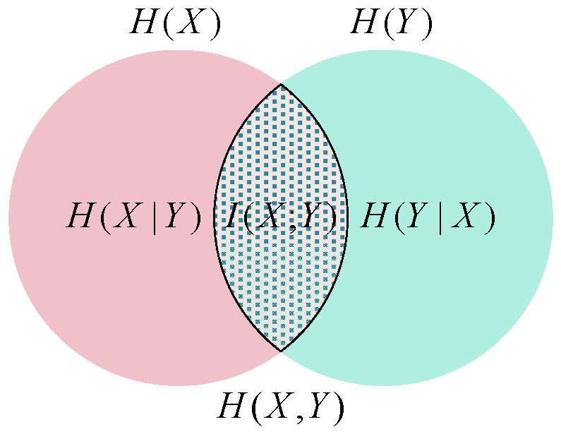Currently, the mainstream data dimensionality reduction methods include unsupervised dimensionality reduction algorithms and feature selection algorithms; compared to the former, the latter only filters the existing features, which has the advantage of strong interpretability [12]. Mutual information (MI) has been widely used as a simple and efficient feature selection algorithm [13,14,15]. For example, Jiang et al. proposed a multi-block principal component analysis method based on MI and utilized SVDD to comprehensively evaluate the monitoring results of all sub-blocks to achieve anomaly detection in industrial process monitoring [16].

The main task of fault detection for mechanical equipment is that the model can identify the abnormal behavior of the equipment through real-time data. However, the fault state of the equipment in the industrial field is highly accidental, so it is quite difficult to collect the abnormal state data, compared with the normal state data that can be easily obtained. Moreover, even if a small amount of fault data is obtained, it is difficult to fully describe all fault states [17,18]. Therefore, the Anomaly Detection (AD) algorithm, that only needs normal data to complete the modeling process, has become the key to solving this problem [19,20]. Moreover, compared with the classification model, the AD algorithm also has great advantages in detecting unknown faults [21]. For example, Yu et al. used MoniNet, an innovative network architecture and analysis methodology, to improve the accuracy and efficiency of industrial process monitoring and control [22]. As a classic algorithm in the AD field, Support Vector Data Description (SVDD) was proposed by Tax et al. [23] in 1999 and has been widely used in biochemistry, cloud computing, fault diagnosis, and other fields [24,25,26]. Since the performance of SVDD is deeply affected by the selection of hyperparameters, various meta-heuristic methods have been used to optimize SVDD hyperparameters [27,28]. However, because SVDD only establishes decision boundaries for normal data, it easily leads to the overfitting of the model and a high false positive rate. For this reason, Tax et al., the creators of SVDD, pointed out in 2004 that adding abnormal data to the training set is expected to strengthen the description of normal data on the decision boundary, and proposed the SVDD with negative examples (SVDD-neg) algorithm [29]. Like SVDD, SVDD-neg relies heavily on hyperparameter tuning. Ni et al. used PSO to optimize the hyperparameters of SVDD-neg and significantly reduced the false positive rate in Foreign Object Damage (FOD) target detection under strong ground clutter [30]. However, the PSO Algorithm is prone to fall into the local optimal solution in the optimization process [31]. Therefore, in this paper, a GA-SVDD-neg algorithm is proposed to optimize the SVDD-neg using GA, which has strong global searching ability, to achieve the abnormal monitoring of hydraulic servomotors.

Finally, based on the principle of warning-then-diagnosis, when the anomaly detection model gives a fault prediction, the classification model realizes the diagnosis of existing faults. In recent years, with the improvement in computing power, deep learning, and especially Convolutional Neural Networks (CNNs), has become a research focus in the field of fault diagnosis [32]. CNNs can automatically extract features, and the feature extraction process is directly oriented to fault classification. This end-to-end joint optimization is conducive to improving the generalization ability of the model. Since Krizhevsky et al. used a CNN to obtain the best classification in the ImageNet Large-scale Visual Recognition Challenge in 2012 [33], CNNs have been widely used in the field of image recognition. Therefore, many scholars have combined the time–frequency transform method with 2DCNN. It is applied for the intelligent fault diagnosis of equipment [34,35]. However, the state signal during machine operation is usually a one-dimensional vector and the time–frequency conversion of the original signal will cause a certain degree of information distortion. 1DCNN directly processes the original one-dimensional time series signal, which not only avoids input information loss but also simplifies the network structure, which is conducive to the application of the model in the real-time diagnosis of equipment.

The main contributions of this research are as follows:

(1)

The MSIF “feature-level” information fusion technique is adopted to stitch the features from different pressure signals into a comprehensive feature, which provides a more comprehensive and in-depth data perspective for the subsequent training of the anomaly detection model. The MI algorithm is also used to remove redundant features in the fused high-dimensional features, which enhances the robustness and generalizability of the subsequent model.

(2)

A GA-SVDD-neg algorithm is proposed by optimizing SVDD-neg using GA with strong global search capability, and the accuracy of the GA-SVDD-neg model is directly used as a quantitative index to evaluate the performance of the feature selection algorithm, which implements the MI-GA-SVDD-neg joint optimization. The superiority of MI-GA-SVDD-neg is verified by combining and co-optimizing four feature dimensionality reduction methods with GA-SVDD-neg, which are Principal Components Analysis (PCA), minimum Redundancy–Maximum Relevance (mRMR), Analysis of Variance (ANOVA), and Random Forest-based Recursive Feature Elimination (RFE).

(3)

The superiority of GA-SVDD-neg compared to PSO-SVDD and GA-SVDD is verified based on the feature set screened by MI.

(4)

1DCNN was employed for pattern recognition of the hydraulic servomotor and the effectiveness of the algorithm in the fault diagnosis of the hydraulic servomotor was verified.

The rest of the paper is organized as follows. Section 2 summarizes the basic principles of MI and SVDD-neg algorithms. Section 3 analyzes in detail the process of collecting experimental data and constructing feature sets. Section 4 conducts comparative experiments and analyzes the main results. Section 5 analyzes the results of the 1DCNN test. Finally, the conclusions are summarized and future research is envisioned in Section 6.

2. Related Technologies and Theories

2.1. Mutual Information

MI is a measure of the degree of interdependence between random variables, $X$ and $Y$. It indicates the extent to which the uncertainty in $X$ is reduced when $Y$ is known, and is given by the following formula:

$$I(X;Y)=\sum _{x\in X}\sum _{y\in Y}p(x,y)\log \frac{p(x,y)}{p(x)p(y)}$$

(1)

The relationship and difference between MI and information entropy are shown in Figure 1. The correlation of the two random variables increases with the increase in their mutual information value, so MI can be used as a measure of the amount of information shared by two random variables. The specific expression of MI is as follows:

$$\begin{array}{c}I(X;Y)=\\ H(X)-H(X\mid Y)=\\ H(Y)-H(Y\mid X)=\\ H(X)+H(Y)-H(X,Y)\end{array}$$

(2)

where $H(X)$ and $H(Y)$ are the entropies of random variables $X$ and $Y$, respectively. $H(X,Y)$ is the joint entropy, which represents the joint distribution of two random variables $X$ and $Y$. Conditional entropy $H(X|Y)$ represents the uncertainty of random variable $X$ when random variable $Y$ is known. In machine learning tasks, MI is used as a measure of the correlation between features and labels and is used to screen out features with a strong correlation with labels to achieve the purpose of feature selection.

2.2. Principle of SVDD-neg Algorithm

Figure 2 shows the basic classification of SVDD. In the figure, the solid circles are the target class samples that need to be described, and the cross symbols are the anomaly samples that need to be rejected; $S$ is the spherical boundary of the described region. SVDD is the coverage area determined by defining the center $a$ and radius $R$ of the sphere, and rejecting the abnormal class sample as much as possible while completely covering the target class sample, and the relaxation variable ${\xi }_i$ is used to reduce the influence of outliers on SVDD. However, the decision boundary of SVDD is often not tight enough, and some abnormal samples are easily misjudged as normal samples, so the generalization of the model is low. To make up for this deficiency, Tax et al. introduced abnormal samples into the training process of the model and proposed the SVDD-neg algorithm. The mathematical model of SVDD-neg can be expressed as follows:

$$\begin{array}{l}\underset{R,a}{\min }{R}^2+c_1{\displaystyle \sum _{i=1}^n}{\xi }_i+c_2{\displaystyle \sum _{l=1}^m}{\xi }_l,\hspace{1em}{\xi }_i,{\xi }_l\ge 0\\ \mathrm{s}.\mathrm{t}.{\Vert \varphi \left(x_i\right)-a\Vert }^2\le R^2+{\xi }_i,\hspace{1em}{y}_i=1\\ {\Vert \varphi \left(x_l\right)-a\Vert }^2\ge R^2-{\xi }_l,\hspace{1em}{y}_l=-1\end{array}$$

(3)

where ${\left\{x_i,y_i\right\}}_{i=1}^n$ is the target class sample set, $y_i=+1$ is the label of $x_i$, ${\left\{x_l,y_l\right\}}_{l=1}^m$ is the sample set of exception class, $y_l=-1$ is the classification identifier of $x_l$, $c_1$ and $c_2$ are penalty factors, and ${\xi }_i$ and ${\xi }_l$ are relaxation factors. Using the Lagrange principle to solve the above optimization problems, there are

$$\begin{array}{c}L\left(R,a,{\xi }_i,{\xi }_l,{\alpha }_i,{\alpha }_l,{\beta }_i,{\beta }_l\right)=R^2+c_1{\displaystyle \sum _{i=1}^n}{\xi }_i+c_2{\displaystyle \sum _{l=1}^m}{\xi }_l-{\displaystyle \sum _{i=1}^n}{\beta }_i{\xi }_i-{\displaystyle \sum _{l=1}^m}{\beta }_l{\xi }_l\\ -{\displaystyle \sum _{i=1}^n}{\alpha }_i\left[R^2-\varphi \left(x_i\right)-a^2+{\xi }_i\right]-{\displaystyle \sum _{l=1}^m}{\alpha }_l\left[\varphi \left(x_l\right)-a^2-R^2+{\xi }_l\right]\end{array}$$

(4)

where ${\alpha }_i\ge 0$, ${\alpha }_l\ge 0$, ${\beta }_i\ge 0$, and ${\beta }_l\ge 0$. The final distance from any test sample $z$ to the center of the sphere $D$ is obtained as follows:

$$D=\sqrt{K\left(z,z\right)-2{\displaystyle \sum _{i=1}^n{\alpha }_i^{\prime }K\left(z,x_i\right)+{\displaystyle \sum _{i=1}^n{\displaystyle \sum _{j=1}^n{\alpha }_i^{\prime }{\alpha }_{j}K\left(x_i,x_j\right)}}}}$$

(5)

where ${\alpha }_i^{\prime }=y_i{\alpha }_i$ and $x_j$ are of the same class as $x_i$. If $D\le R$, this means that the test sample is on or inside the hypersphere and belongs to the normal sample, $(y=+1)$; if $D>R$, the test sample belongs to the abnormal sample, $(y=-1)$.

Based on the optimal set of special features screened by MI, and also to obtain the SVDD model with a better generalization performance, this paper utilizes the SVDD-neg algorithm to achieve the anomaly detection of an adjustment hydraulic servomotor.

3. Experiment Settings

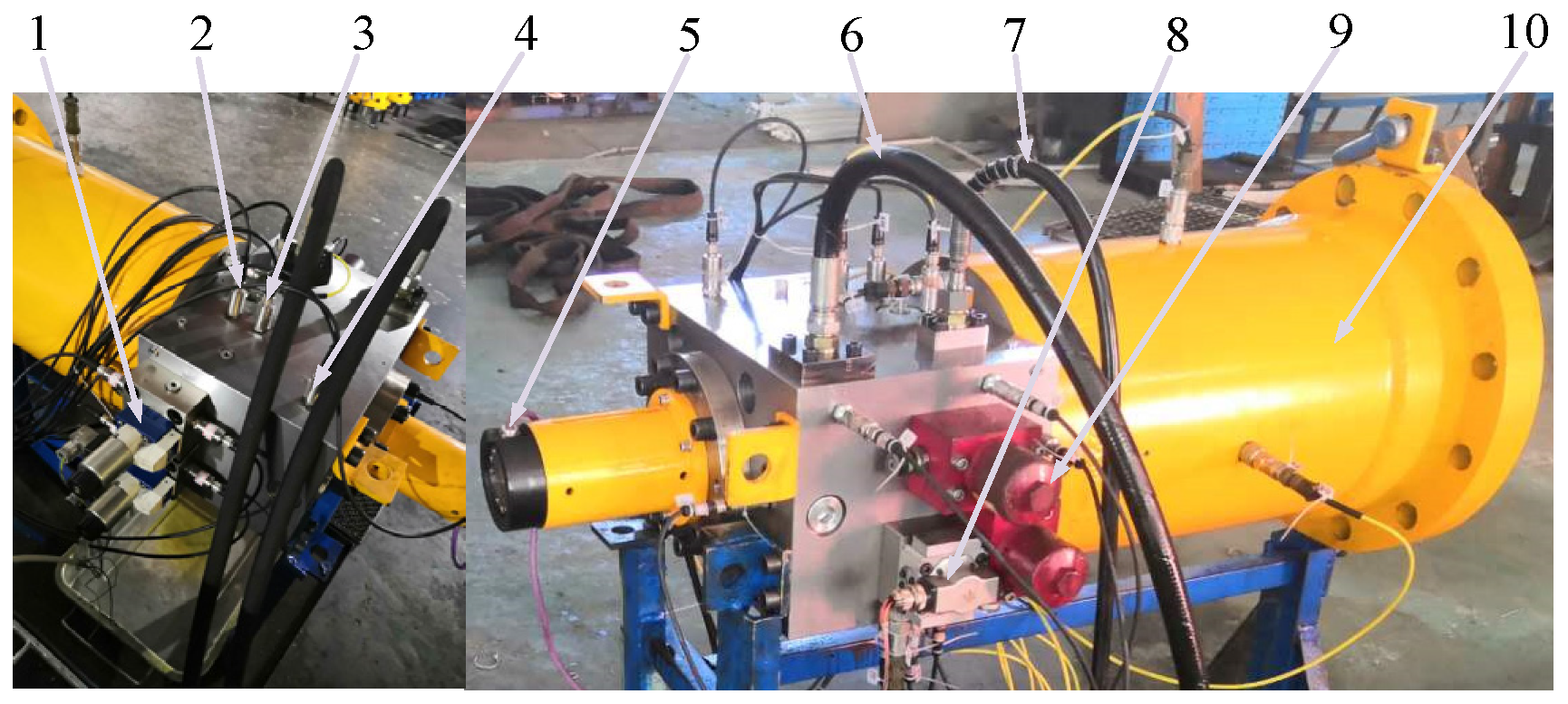
This paper designs and conducts relevant tests using the high-pressure adjustment hydraulic servomotor fault simulation test bench, as depicted in Figure 3. The structure of the high-pressure adjustment hydraulic servomotor is a symmetrical cylinder with one-sided action. It is composed of a spring, cylinder, electro-hydraulic servo valve, throttle hole, oil filter, displacement, pressure sensor, electrical junction box, and valve block for installing a quick-closing solenoid valve and inserted one-way valve. A pressure sensor M3 is installed between the non-working chamber of the adjustment hydraulic servomotor and the port B of the cartridge valve, pressure sensor M4 is installed between the throttle hole C0 and the working chamber of the adjustment hydraulic servomotor, and pressure sensor M5 is installed between the throttle hole D0 and the port A of the cartridge valve. All three are installed by threaded holes.

Since the original three pressure sensors M3–M5 and one displacement sensor LVDT cannot fully obtain system state information, this paper optimizes the layout of the measuring points by adding 5 new measuring points P5–P9 for pressure measurement based on the original measuring points. P5 is installed at the oil inlet of the system, P6 is installed at the working port of electro-magnetic directional valve 1 (left), P7 is installed at the working port of electromagnetic directional valve 2 (right), P8 is installed at the oil inlet of electromagnetic directional valve 1 (left), and P9 is installed at the oil inlet of electromagnetic directional valve 2 (right). After that, this study realized the fault implantation of the adjustment hydraulic servomotor by replacing the faulty components or artificially destroying the normal parts. A total of six fault states were set, including in-cylinder leakage, spring breakage, solenoid valve throttle orifice blocked, spool zero position internal leakage, solenoid valve internal leakage, and C0 throttle orifice clogged. The sensors’ layout design and the six fault settings are shown in Figure 4. Among them, the leakage in the normal servo valve is 0.70 L/min, and the leakage in the worn servo valve is 12.32 L/min. The solenoid valve internal leakage is simulated by replacing the internal leakage solenoid valve. The normal diameter of the solenoid valve front throttle hole is φ = 0.8 mm, processing and replacing the smaller throttle hole diameter of φ = 0.5 mm; the C0 throttle hole’s normal diameter is φ = 3 mm, processing and replacing the throttle hole diameter of φ = 1 mm. The in-cylinder leakage fault is simulated by wearing the seal ring. The spring breakage fault is simulated by artificially destroying the internal small spring or cutting a part of the spring.

Finally, according to the above six fault states and normal states, the pressure of the EH oil supply system is adjusted to 15 MPa; then, the adjustment hydraulic servomotor is controlled by LabVIEW under the working condition of a frequency of 0.1 Hz and amplitude of 5%. The Machine Condition Monitoring (MCM_2.1.2.0) software was used to set the sampling frequency to 12.5 kHz, each sampling time to 30 s, and each state to be sampled three times.

4. Abnormal Detection of Adjustment Hydraulic Servomotor

4.1. Feature Extraction and Feature Fusion

In this paper, a total of 17 time-domain characteristic parameters, such as mean value and absolute mean value, were extracted to represent the amplitude fluctuation, power fluctuation, and waveform distribution of the signal, respectively. At the same time, this paper also extracted 13 frequency-domain characteristic parameters, such as the mean value of frequency domain amplitude and frequency variance, to characterize the frequency distribution of signals in the frequency domain and the degree of spectrum concentration.

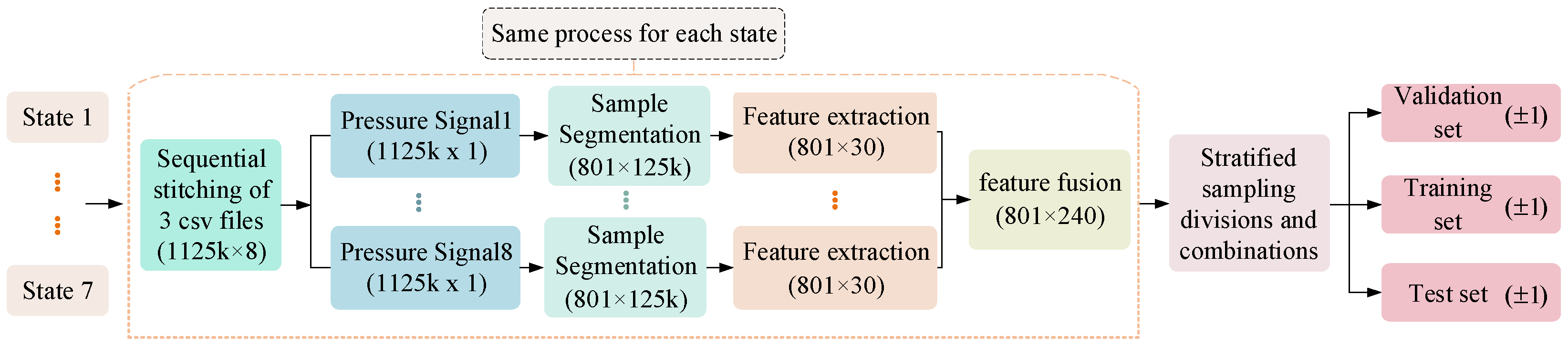
In addition, the sensor information of each spatial position of the equipment is consistent and complementary, and the accuracy and generalization ability of the anomaly detection model can be improved by using multi-sensor fusion technology to synthesize, refine, and optimize the sensor information. According to the different resolutions of data and processing processes, multi-sensor fusion technology can be divided into three categories: data layer fusion, feature layer fusion, and decision layer fusion. The feature layer fusion in the middle layer is to compress the information of the original data through feature extraction, and then fuse it into a comprehensive feature through sequential splicing, which is conducive to online real-time processing. This study pays attention to the effect of the model in practical applications and has high requirements for real-time performance, so “feature layer fusion” is chosen as the information fusion method. The specific process of feature selection and fusion is shown in Figure 5.

Each step in the flow chart is described as follows:

Step 1: Longitudinally concatenate three consecutive data files in seven states, respectively, to obtain seven data files with the shape of (1125k × 8). Then, the data files of the seven states are combined to obtain three-dimensional data with the shape of (7 × 1125k × 8).

Step 2: Separate samples of each state and signal by sliding window. To ensure that the sample contains at least one cycle of device operation data, the window and window stack lengths are set to 125k and 1250, respectively. Thus, the three-dimensional data of (7 × 1125k × 8) are converted to the four-dimensional data of (7 × 8 × 800 × 125k). That is, there are seven states, each state contains eight signals, and each signal generates 800 samples, respectively, and the length of each sample is 125k.

Step 3: Perform feature extraction on the samples obtained in step 2 based on the selected 30 time and frequency domain features and reduce the feature dimension from 125k to 30 to obtain an initial feature sample set (7 × 8 × 800 × 30).

Step 4: Adopting ‘feature level fusion’ technology, the 30-dimensional feature samples of eight pressure signals are spliced horizontally head to tail, resulting in a comprehensive feature sample with a dimensionality of 240, denoted as (7 × 800 × 240) 3-dimensional data. The “normal state” samples were separated, while the six “fault state” samples were combined.

Step 5: Designate the “normal state” sample as the target for the SVDD-neg model with the label set as ‘1’. Divide it into a positive example training set, positive example verification set, and positive example test set using a ratio of ‘3:1:1’ through random sampling division. The number of samples in the positive example training set is 480, the positive example verification set is 160, and the positive example test set is 161.

Step 6: Set integer labels for the six “fault state” samples and divide them into a counter-example training set, counter-example verification set, and counter-example test set using hierarchical sampling division. The number of samples in the counter-example training set is 479, the counter-example verification set is 160, and the counter-example test set is 161. Then, set all counter-example sample labels as ‘−1’.

Step 7: Combine the positive example training set and negative example training set into a mixed training set (label contains both ‘1’ and ‘−l’), combine the positive example verification set and negative example verification set into a mixed verification set, and combine the positive example test set and negative example test set into a mixed test set.

The results of the data set are shown in

Table 1. SVDD experimental data arrangement.

State Type	Tag	Training Set	Verification Set	Test Set	Length of Sample
Normal	1	480	160	161	240
In-cylinder leakage	−1	79	27	27	240
Spring breakage	−1	80	26	27	240
Solenoid valve throttle orifice blocked	−1	80	27	27	240
Spool zero position internal leakage	−1	80	27	27	240
Solenoid valve internal leakage	−1	80	26	27	240
C0 throttle orifice clogged	−1	80	27	26	240

. In the training set, verification set, and test set, not only is the number of positive and negative samples relatively balanced, but the number of abnormal state samples in the negative samples is also balanced. In this way, the SVDD-neg model can be ensured to tighten the decision boundary as much as possible while paying attention to the positive samples and establishing its boundary description.

4.2. Wrapper-Type Feature Selection Based on MI and GA-SVDD-neg

4.2.1. Combined Optimization of MI-GA-SVDD-neg

The high-dimensional data after feature fusion will make the model computation grow exponentially and easily lead to problems of high model complexity and low generalization ability, so it is necessary to reduce the dimensionality of the feature set. By using the feature selection algorithm, we can gain insight into the signal channels and feature names that are sensitive to the state of the device, which is conducive to reducing the number of sensors in the later stage and the promotion of this study to real-world applications. Therefore, in this study, the MI feature selection algorithm is utilized to perform feature screening on the 240-dimensional comprehensive feature set and is combined with the GA-SVDD-neg algorithm as a wrapper-style feature selection algorithm to jointly optimize the MI-GA-SVDD-neg.

Firstly, dimension reduction was performed on the training set, verification set, and test set using the MI algorithm. It is assumed that, after dimensionality reduction, all three data sets have a reduced dimensionality denoted as “$m$” ($m\in A,A=\left\{n|1\le n\le 240\right\}$). Subsequently, training, validation, and hyperparameter optimization were conducted using the GA-SVDD-neg model on $m$-dimensional training sets and verification sets. The accuracy value of the optimal model on $m$-dimensional test sets was then calculated as a quantitative indicator “$b$” for evaluating compatibility between “the $m$-dimensional feature set proposed by MI” and “GA-SVDD-neg”. The specific process of optimizing the SVDD-neg hyperparameter by GA is described. The hyperparameters of the SVDD-neg algorithm consist of the positive case penalty factor ($c_1$) and the negative case penalty factor ($c_2$). Additionally, a radial basis kernel function is utilized to address the issue of linear indivisibility in the data. 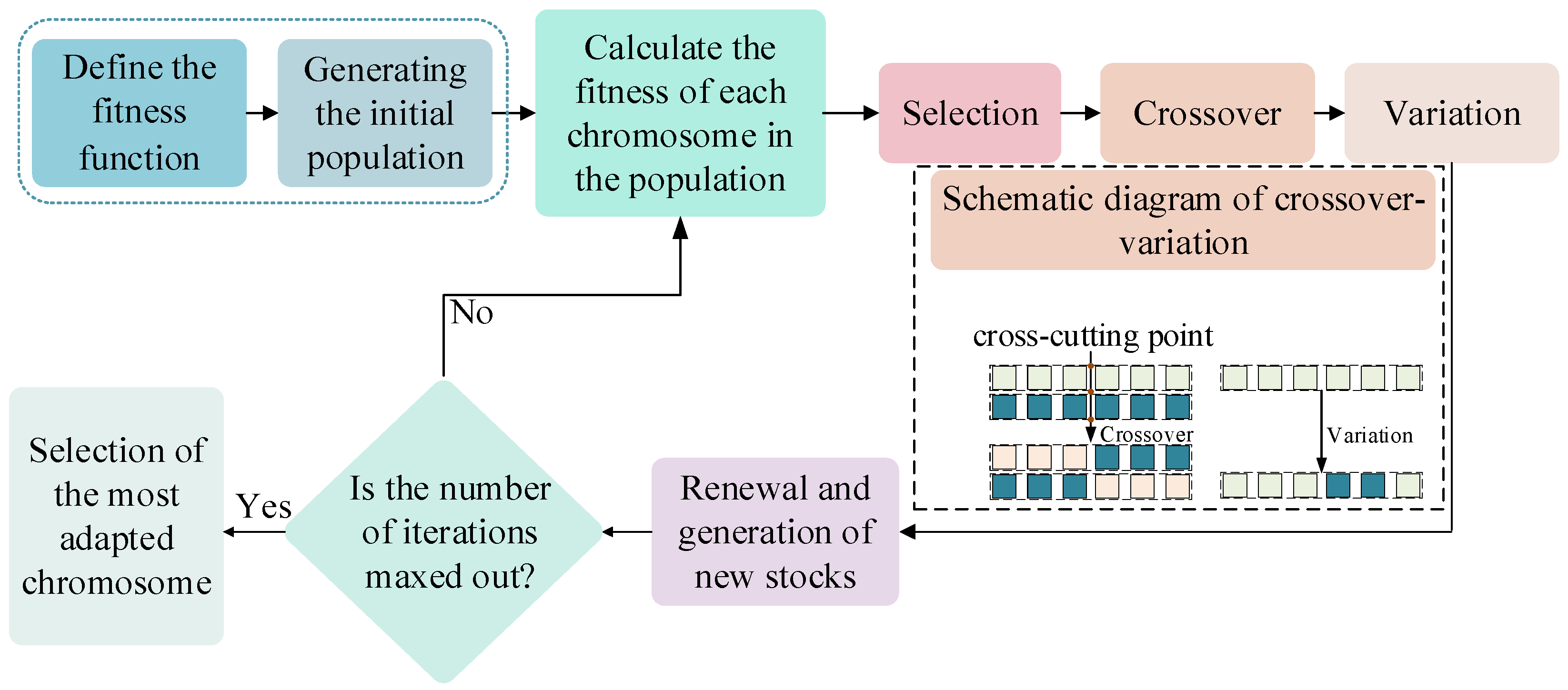Therefore, the GA needs to optimize three hyperparameters including the radial basis kernel function parameter $\gamma$ at the same time. The implementation of the GA-SVDD-neg algorithm proposed in this study is shown in Figure 6:

Step 1: Define the fitness function of the GA algorithm. Assume that the accuracy of the SVDD-neg model on $m$-dimensional verification set is $a$, then define the fitness value of the GA algorithm as $(1-a)$, and the iterative goal of the GA algorithm is to minimize the fitness value of chromosomes in the $m$-dimensional verification set.

Step 2: Binary code a hyperparameter combination ($c_1$,$c_2$,$\gamma$) into a chromosome, where $c_1$, $c_2$, $\gamma$ all have values in the range [0.001, 1]. Then, the initial population with 50 chromosomes is randomly generated, and the maximum number of iterations is set to 10, and the mutation probability is set to 0.001.

Step 3: Initialize the SVDD-neg model based on the chromosomes in the population; then, train the model on the $m$-dimensional training set and obtain the fitness value of each chromosome on the $m$-dimensional validation set.

Step 4: Select chromosomes to enter the next generation population according to the fitness value of chromosomes; at the same time, cross and mutate chromosomes according to certain strategies and add the newly generated chromosomes to the next generation population. Then, renew and create new populations.

Step 5: Determine whether the maximum number of iterations has been reached. If no, return to Step 3. If yes, proceed to Step 6.

Step 6: Calculate and select the chromosome with the highest fitness value in the new population and initialize the SVDD-neg model after decoding it into a combination of hyperparameters. Finally, the model was retrained on the $m$-dimensional training set + validation set, and the accuracy value of the model was calculated on the test set.

4.2.2. Comparative Study of Feature Selection Algorithms

To highlight the superiority of the MI-GA-SVDD-neg joint optimization algorithm, this study adopts the same wrapper feature selection idea to combine and similarly co-optimize the GA-SVDD-neg with the four dimensionality reduction methods of ANOVA, MRMR, RFE, and PCA, respectively, to conduct a comparative study.

The specific comparative research process is shown in Figure 7:

Step 1: Select a dimensionality reduction method from five dimensionality reduction algorithms.

Step 2: Use the selected method to reduce the feature dimension to $m$ and calculate the evaluation indicator $b$.

Step 3: Increase $m$ from 1 to 240 and repeat step 2 until $m$ = 240.

Step 4: Repeat steps 1 to 3 until all feature dimensionality reduction algorithms have been traversed.

Step 5: Summarize and plot an analysis of $b$, as shown in Figure 8.

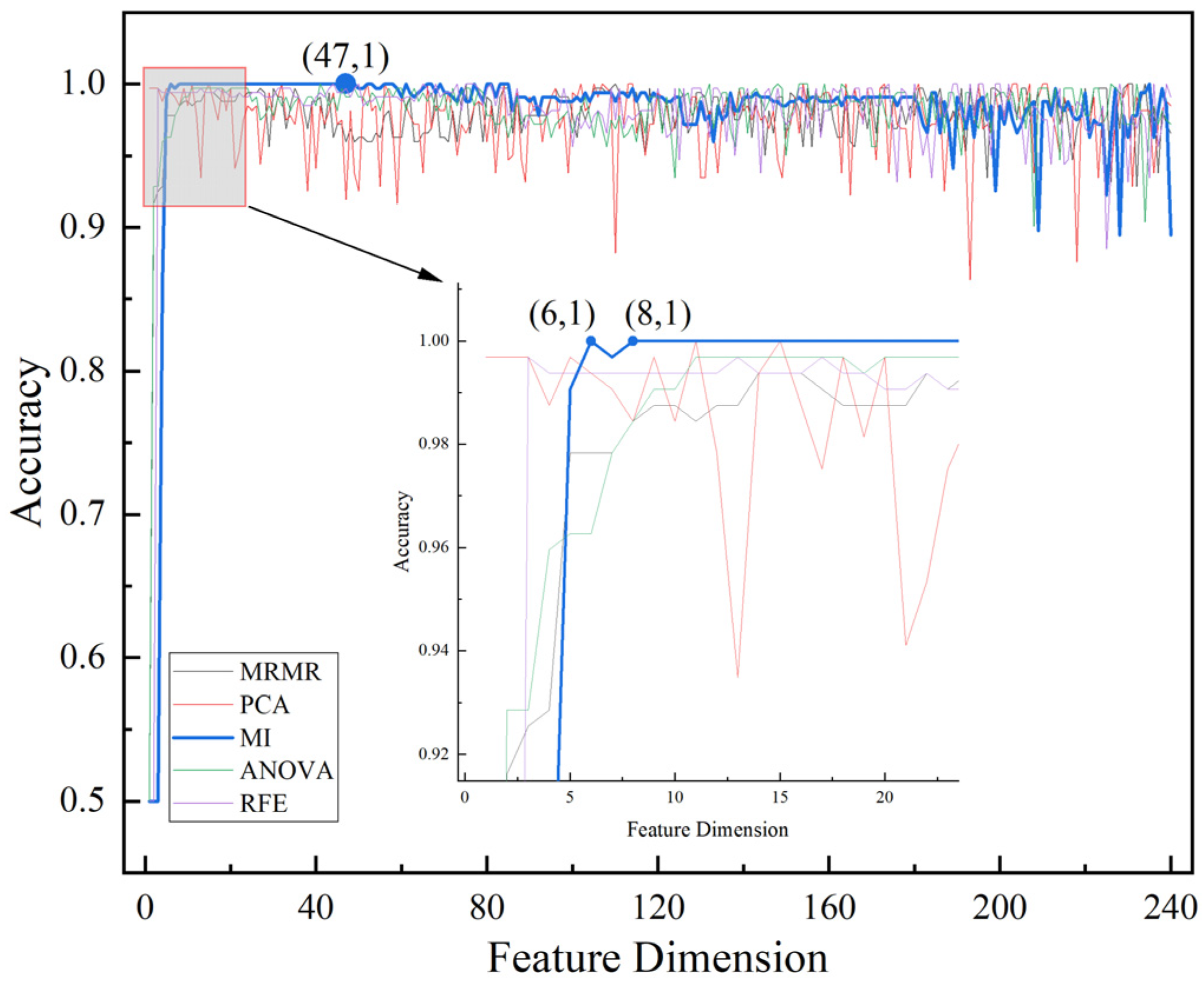
From Figure 8, it can be seen that the effect of the GA-SVDD-neg model begins to deteriorate as the feature dimension rises and shows increasingly violent oscillations, indicating that the high-dimensional features do contain redundant features. For the distance-based SVDD-neg model, the existence of redundant features will lead to the problem of data sparsity in the high-dimensional feature space, which increases the risk of model overfitting and makes the model more sensitive to small data changes, thus reducing the stability of the model, which reflects the necessity of “feature selection”.

For a certain feature dimension reduction method $i$, if the feature dimension is reduced to $m$ by the $i$ method and the evaluation indicator $b=100\%$, then the current $m$ is identified as a good feature dimension and defined as $m_i$. Assuming that all $m_i$ of the $i$ method constitute a good dimension set $B$ ($B\subseteq A$), then the higher number of elements in set $B$ represents the higher robustness of the GA-SVDD-neg model to the $i$ algorithm. Further, a comparative study of these dimensionality reduction methods allows the selection of the most robust feature reduction algorithm and its corresponding optimal feature dimension $k$, $k=B_{\min }$. Accordingly, it can be seen from the analysis of Figure 8 that, on the one hand, when the number of feature selections increases from 8 to 47, the feature set selected based on MI algorithm can make the accuracy of GA-SVDD-neg model reach 100%, indicating that the GA-SVDD-neg model has the strongest robustness to the MI algorithm; on the other hand, the MI algorithm only needs to select six features to make the accuracy of the GA-SVDD-neg reach 100%, indicating that, compared with other algorithms, the MI algorithm preferentially selects the features most suitable for the GA-SVDD-neg model.

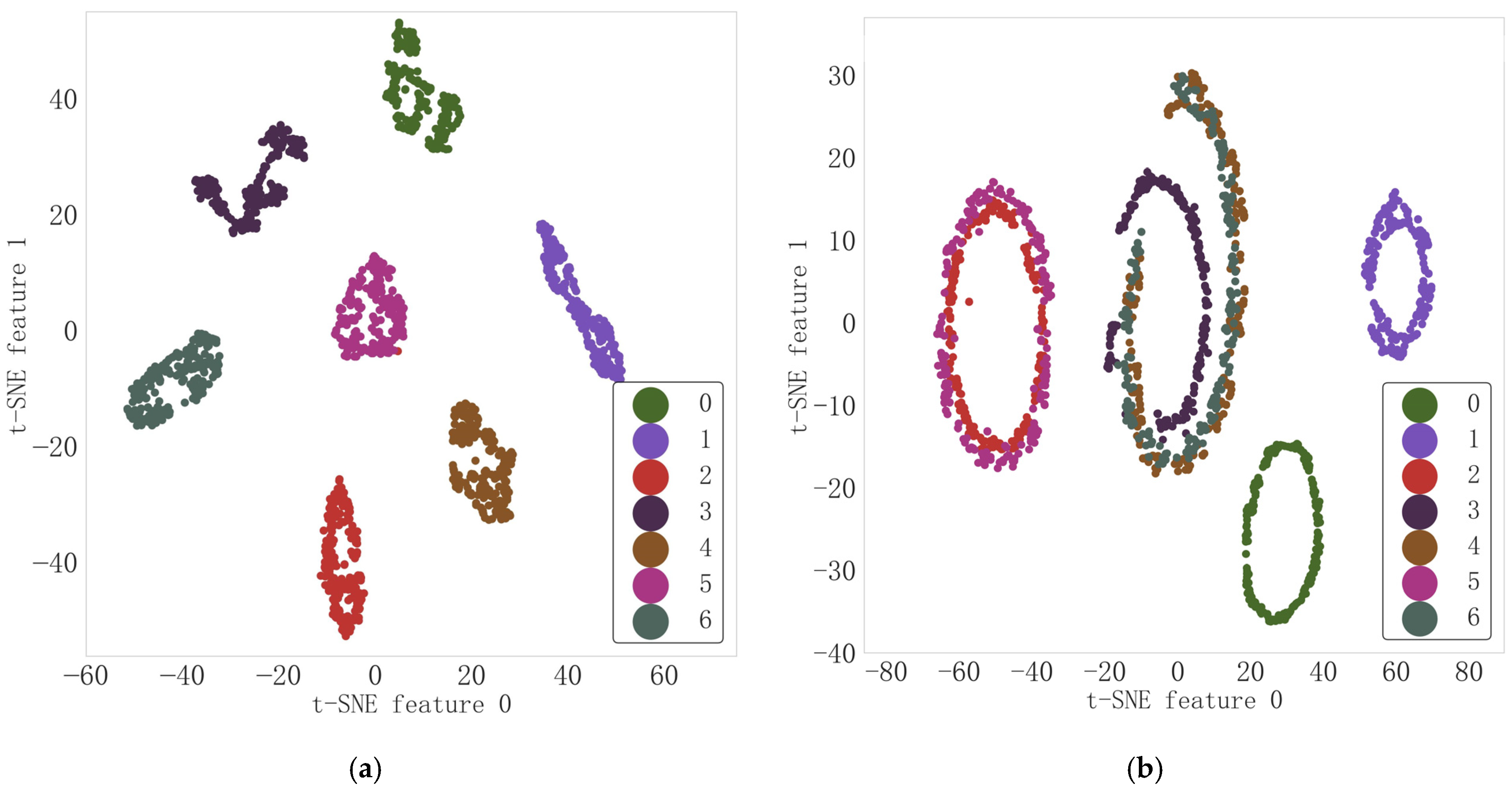
To further verify the effectiveness of the six features proposed by “mutual information” and the applicability of this feature set with GA-SVDD-neg, on the one hand, this paper uses the t-Distributed Stochastic Neighbor Embedding (t-SNE) dimension reduction algorithm to reduce and visually analyze the original 240-dimensional features and the 6-dimensional features proposed by MI, respectively. Figure 9a shows a obvious overlap phenomenon between normal and abnormal samples in the spatial distribution of the 240 dimensional feature set, while Figure 9b shows a significant difference in the spatial distribution of normal and abnormal samples in the 6-dimensional feature set. On the other hand, this paper uses the GA algorithm to optimize SVDD-neg 30 times in the 6-dimensional feature set and 240-dimensional feature set, respectively, and the optimization process each time is the same as the calculation process of GA-SVDD-neg described in Section 4.2.1. Finally, the 30 accuracy values corresponding to the two feature sets are plotted in Figure 9c. The accuracy of GA-SVDD-neg is above 99.5% in 30 tests based on a six-dimensional feature set, and most of them can reach 100%. However, the accuracy of GA-SVDD-neg fluctuates greatly in 30 tests for 240-dimensional features, only reaching 100% five times, and even only 92.857% in the 20th test. The above results are consistent with the conclusion in Figure 8 that “the existence of redundant features in high-dimensional features will lead to the deterioration of the stability of GA-SVDD-neg model”, and also prove that the six features selected by MI have strong applicability and robustness with the GA-SVDD-neg algorithm. Based on this, this paper finally selects the MI method for feature selection and selects six sensitive features of the P9 pressure signal, such as variation rate, frequency variance, waveform index, peak value, square root amplitude, and effective value.

4.2.3. Comparison of Model Training and Testing Time

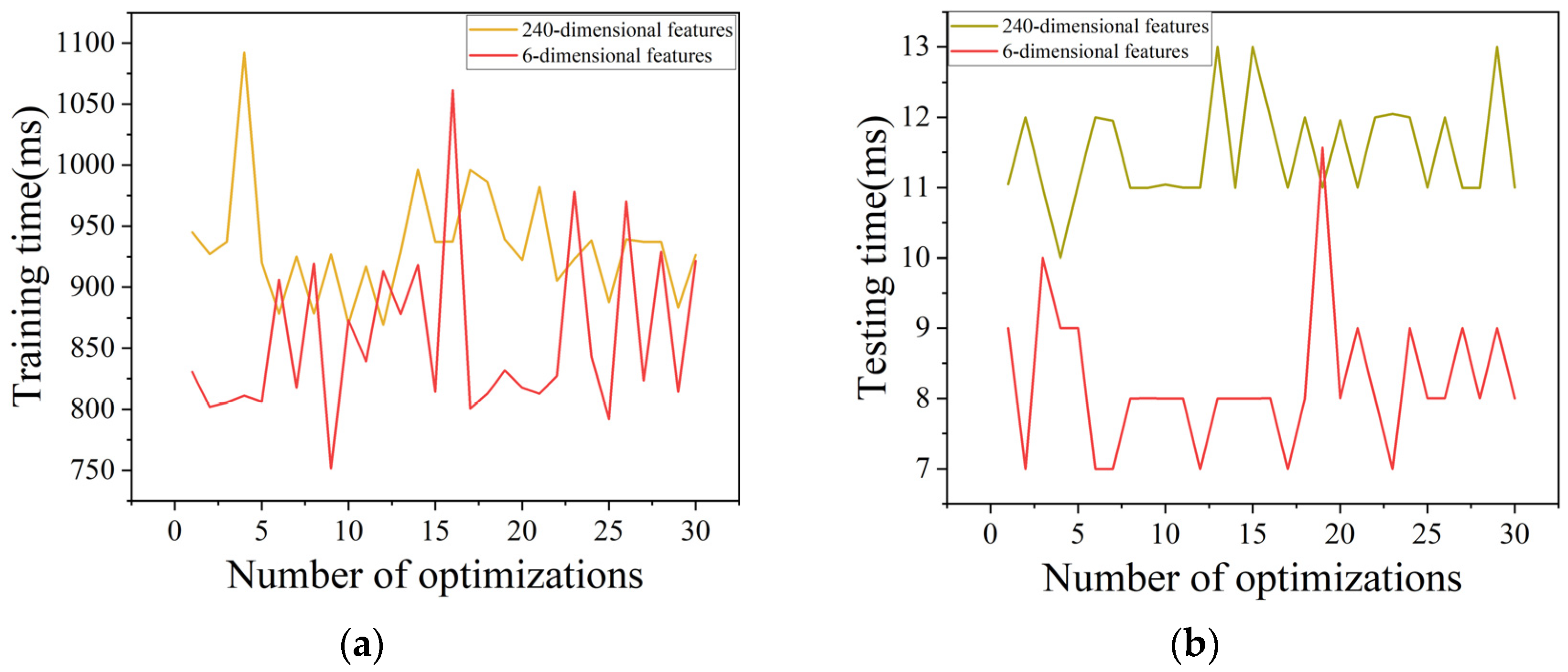
In addition, “feature selection” can not only improve the generalization of the model but also reduce the training and testing time of the model, which is of great significance for the application of the SVDD-neg model. In this paper, the model of GA-SVDD-neg algorithm 30 times optimization is analyzed. The training time on the “training set + verification set” and the test time on the “test set” are summarized, as shown in Figure 10. Compared with the 240-dimensional feature, the training time and test time of SVDD-neg on the 6-dimensional feature are both reduced, and the reduction in the test time is more obvious. This is very conducive to the deployment of the model in real-time fault detection. The average, minimum, and maximum values of the training and testing times of the statistical model are shown in

Table 2. Comparison of training time and test time for two feature sets.

Characteristic Dimension	Label	Training + Verification Set	Test Set	Training Time (s)			Test Time (s)
				Mean Value	Minimum Value	Maximum Value	Mean Value	Minimum Value	Maximum Value
240 dimensions	1	640	161	0.93304	0.86917	1.09226	0.0115	0.01	0.013
	−1	639	161
6 dimensions	1	640	161	0.85739	0.75157	1.06117	0.00822	0.007	0.01157
	−1	639	161

. According to the statistical indicator of “average”, the training time is reduced by about 8.1%, 76 ms, and the test time is reduced by about 28.5%, 3 ms. Considering that the order of training and testing time of the model is small, this degree of reduction effect is already incredibly significant. The experimental analysis of this study was completed on the same computer, which was configured as Intel Core i5-12400F (2.50 GHz), 32 GRAM, and NVIDIA GeForce RTX 3060Ti (8 GB). The development environment was scikit-learn 0.24.2+python 3.6.2 and tensorflow-gpu2.10.0+python 3.8.18.

4.3. GA-SVDD-neg Analysis of Abnormal Detection Results

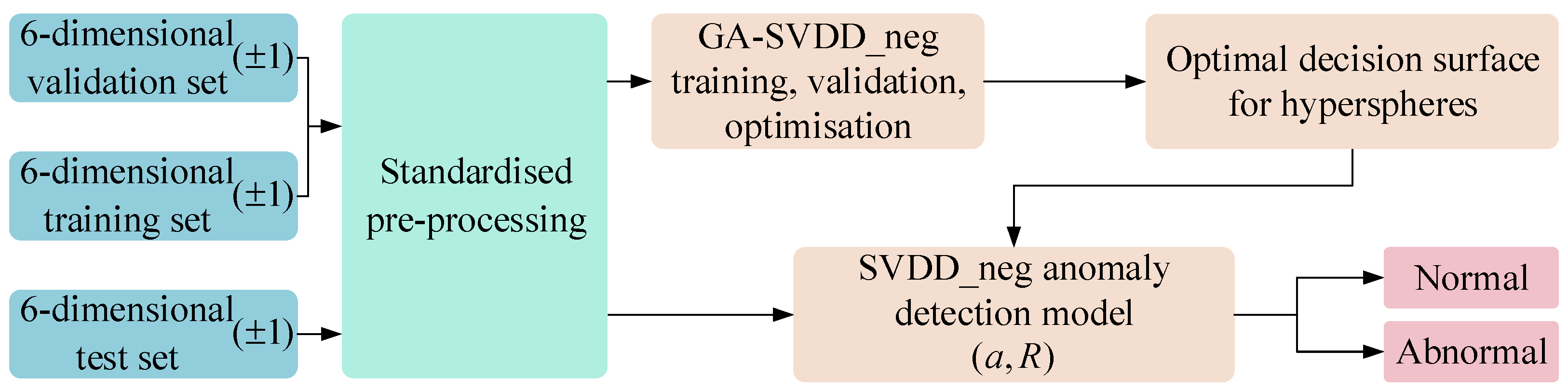
The GA-SVDD-neg fault detection process is shown in Figure 11. In this paper, for the six-dimensional training, validation, and test sets obtained from MI, the three datasets are firstly pre-processed in a standardized way, and the SVDD-neg is trained, optimized, and tested according to the GA-SVDD-neg optimization process described in Section 4.2.1. The hyperparameters of the final SVDD-neg model are shown in

Table 3. Final SVDD-neg model hyperparameter.

Parameter Name	Penalty Factor ${\mathit{c}}_1$	Penalty Factor ${\mathit{c}}_2$	Radial Kernel Parameters $\mathit{\gamma }$	Support Vector Count	Percentage of Support Vectors	Hypersphere Radius
Parameter value	0.93561615	0.72095632	0.97008421	3	0.2346%	0.400601

.

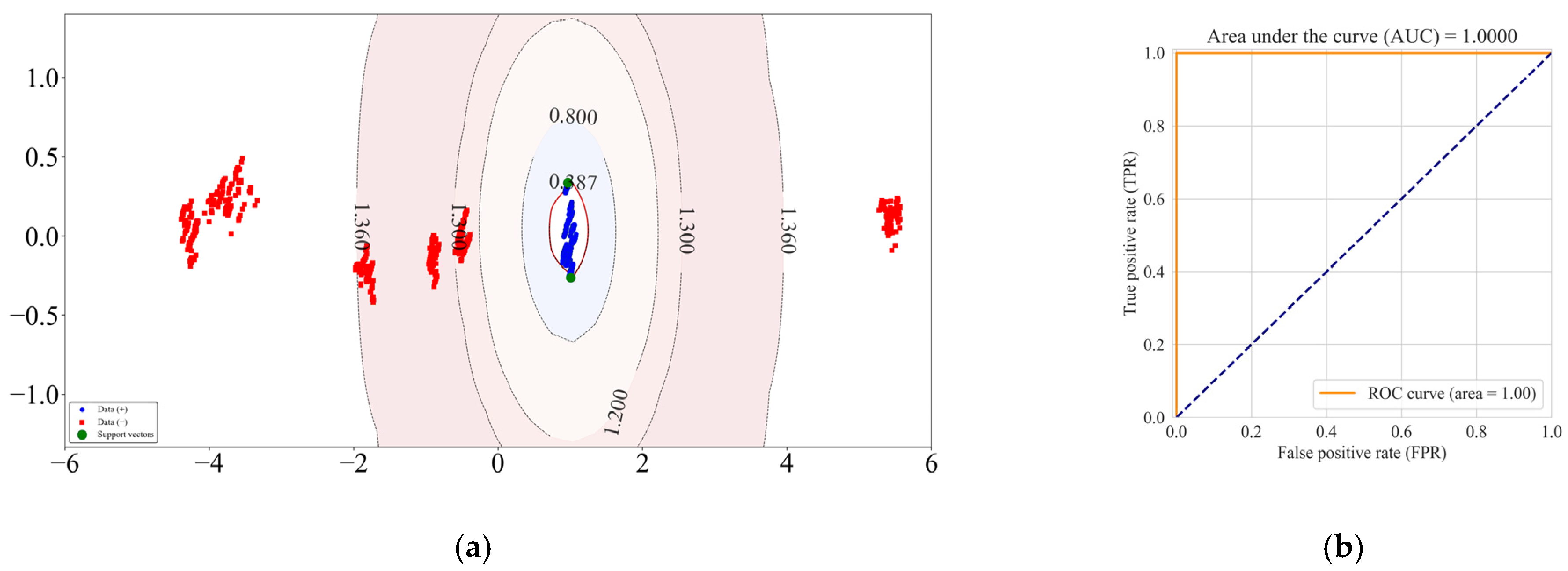
To visually display the “decision boundary” formed by the SVDD-neg model after the training process, the PCA algorithm was used in this paper to reduce the six-dimensional collection to two dimensions and then train and optimize the GA-SVDD-neg model, and the decision boundary of the model was finally drawn, as shown in Figure 12a. The model can not only correctly distinguish normal and abnormal samples, but also clearly distinguish six fault types on the “distance” scale, which verifies the applicability of the SVDD-neg model in the field of the abnormal detection of an adjustment hydraulic servomotor. Figure 12b shows the ROC curve of the current SVDD-neg model on the test set. An AUC of 1 indicates that the effect of the current SVDD-neg model has reached the optimal level and there is no need to further optimize the model, which verifies the superiority of GA in optimizing SVDD-neg hyperparameters.

4.4. A Comparative Study of Anomaly Detection Algorithms

To verify the superiority of the GA-SVDD-neg algorithm proposed in this paper in the field of the abnormal detection of an adjustment hydraulic servomotor, it was compared with GA-SVDD and PSO-SVDD. According to the six features mentioned in Section 4.2.2, the MI algorithm was used in this study to reduce the normal sample training set and verification set divided in Step 5 of Section 4.1 to six dimensions, respectively, for the training and optimization of GA-SVDD and PSO-SVDD models. The test set remained the same as GA-SVDD-neg. After several iterations of optimization, this paper presents the optimal test results of the three algorithms, as shown in Figure 13.

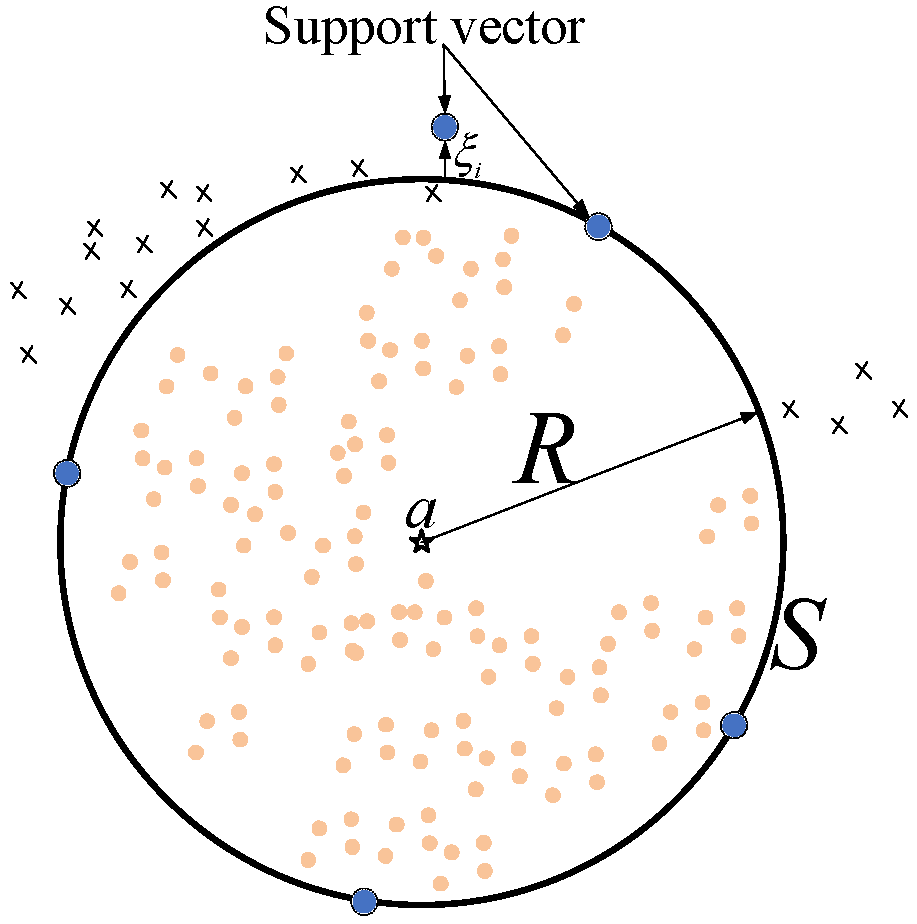
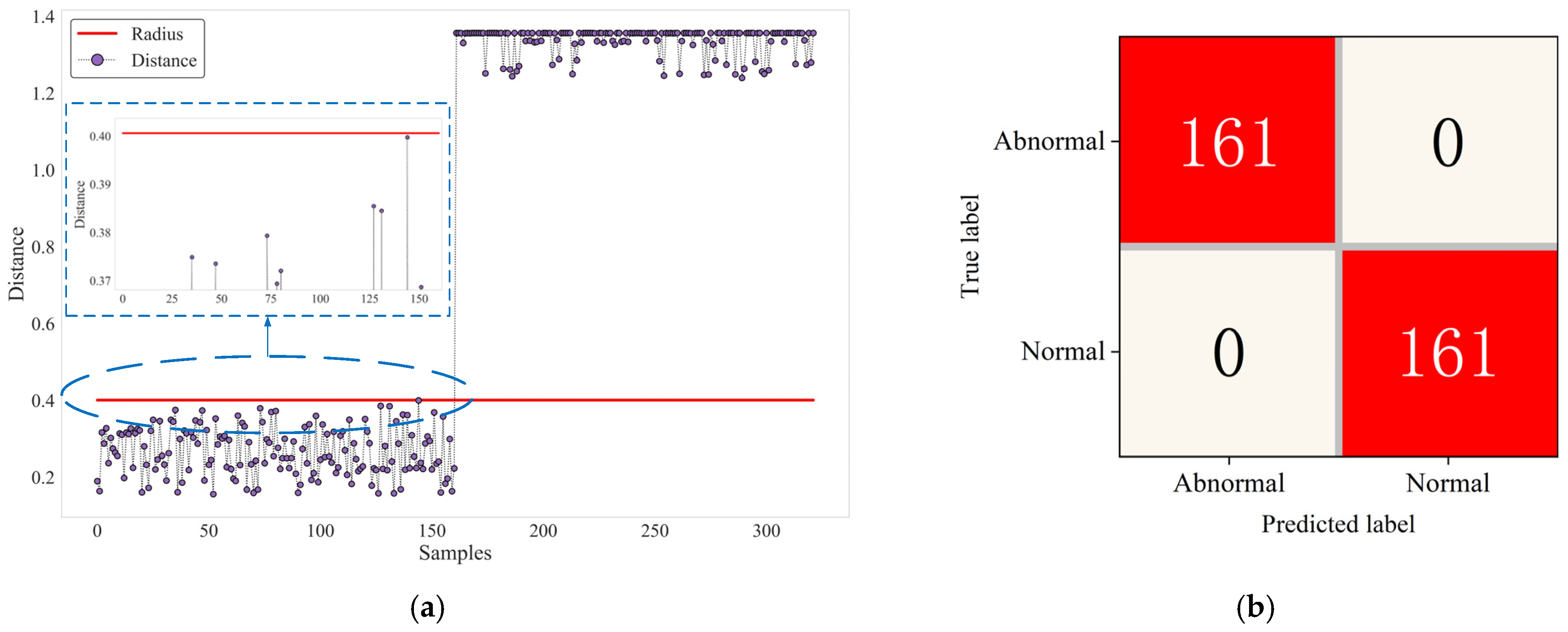
It can be seen from Figure 13a that the distance from the normal samples to the center of the hypersphere is all less than the radius; that is, the GA-SVDD-neg model determines all normal samples as normal. The distance from the abnormal samples to the center of the hypersphere is much larger than the radius; that is, the GA-SVDD-neg model not only determines all abnormal samples as abnormal but also has a strong difference between the distance distribution of abnormal samples and normal samples. The confusion matrix in Figure 13b shows that the accuracy and recall indicator values of the model on the test set both reach 100%, which reflects the powerful generalization ability of the GA-SVDD-neg algorithm. 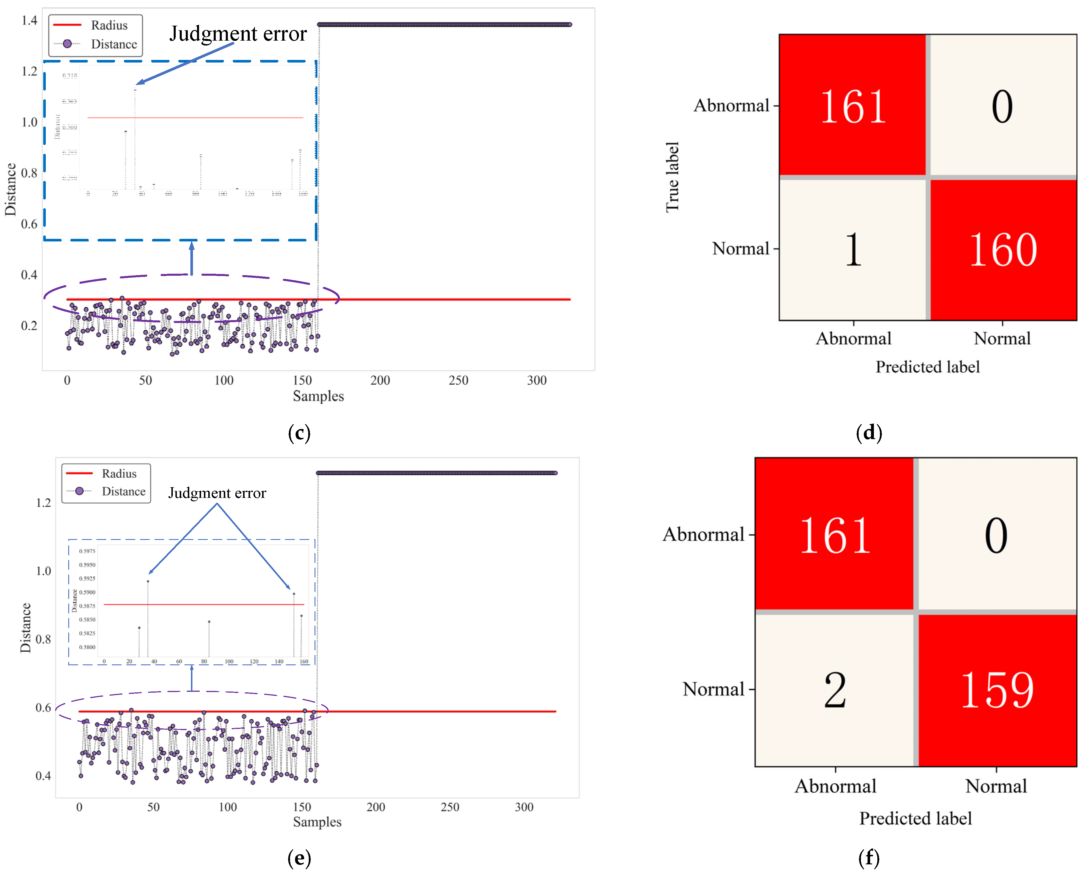Figure 13c,d show that, in GA-SVDD, all abnormal samples are correctly identified, but one normal sample is misjudged as abnormal. Figure 13e,f show that, in PSO-SVDD, all abnormal samples are correctly classified, but two normal samples are misjudged as abnormal samples. The results show that GA-SVDD-neg has a stronger generalization ability than GA-SVDD and PSO-SVDD, and GA is more suitable for the optimization of SVDD hyperparameters than PSO. In this paper, the accuracy rate, recall rate, F1 score, and overall accuracy indicator statistics of the three models on the test set are shown in

Table 4. The results of the three algorithms.

Method	GA-SVDD-neg				GA-SVDD				PSO-SVDD
Indicators/%	Precision	Recall	F1-Score	Accuracy	Precision	Recall	F1-Score	Accuracy	Precision	Recall	F1-Score	Accuracy
Normal	100	100	100	100	100	99.38	99.69	99.69	100	98.76	99.38	99.38
Abnormal	100	100	100		99.38	100	99.69		98.77	100	99.38

:

It can be seen from the above table that GA-SVDD-neg is superior to GA-SVDD and PSO-SVDD in terms of each indicator value. The results show that, when there are negative examples, the GA-SVDD-neg algorithm can be used for anomaly detection to obtain a model with stronger generalization and robustness, and effectively reduce the false positive rate of the model. It is of great significance to the application and popularization of the model in the industrial scene.

5. Fault Diagnosis of Adjustment Hydraulic Servomotor Based on 1DCNN

5.1. DCNN Structure Design

After the adjustment hydraulic servomotor is judged to be faulty by the GA-SVDD-neg model, it is necessary to determine the fault location and fault type. In this paper, based on 1DCNN, the characteristics of pressure signals were automatically extracted and classified, and an end-to-end fault diagnosis model for the adjustment hydraulic servomotor was constructed. Finally, the pattern recognition and fault diagnosis of six fault states and normal states of the adjustment hydraulic servomotor are realized.

The structure and parameters of the 1DCNN model designed in this paper are shown in Figure 14, which includes three parts: the input layer, feature extraction layer, and classification layer. First, the original signal is segmented and transmitted directly to the input layer. The three convolutional layers are then arranged in alternating rows with each of the three pooling layers, which together constitute the feature extraction layer. Among them, the convolution layer uses multiple convolution kernels to extract the original pressure signal of the input layer, and the pooling layer reduces the dimension of the feature vector by the maximum pooling operator while making these features insensitive to translation, offset, and small distortion. After that, all feature vectors are reorganized into one-dimensional vectors by adding the Flatten layer after the third pooling layer, and Dropout is added to prevent overfitting. Finally, a classification layer composed of three fully connected layers is added, and the classification output is performed by the Softmax classifier.

5.2. Data Acquisition and Parameter Setting

According to the results of the MI feature selection algorithm in Section 4.2.2, the P9 pressure signal containing the most sensitive features is selected as the data source of the 1DCNN model. In this paper, a window of 1024 length is used to slice the P9 signals of each state, and it is marked with integer labels. A total of 7000 samples were obtained for seven states, of which 1000 samples were obtained for each state and the sample dimension was 1024. Finally, according to the ratio of 3:1:1, 7000 samples are divided into training sets, verification sets, and test sets via “stratified sampling division”. The details of the 1DCNN experimental data set are shown in

Table 5. 1DCNN experimental data arrangement.

Categories	Labels	Training Set Size	Validation Set Size	Test Set Size
Normal	0	600	200	200
In-cylinder leakage	1	600	200	200
Spring breakage	2	600	200	200
Solenoid valve throttle orifice blocked	3	600	200	200
Spool zero position internal leakage	4	600	200	200
Solenoid valve internal leakage	5	600	200	200
C0 throttle orifice clogged	6	600	200	200

.

After adjusting the model parameters several times and comparing and analyzing the training effect, the relevant settings and parameters of the model were finally determined, as shown in

Table 6. 1DCNN hyperparameter settings.

Parameter Name	Optimiser			Loss Function	Indicator	Epochs	Batch Size	Dropout
	Name	Learning Rate	Decay Rate
Parameter value	RMSProp	0.002	0.9	categorical_crossentropy	accuracy	250	20	0.5

. In this paper, the ReLU activation function and the Dropout technique are used to prevent model overfitting and enhance the robustness of the model. After that, to reduce the dependence on the learning rate scheduler, we chose the RMSprop optimizer that can adaptively adjust the learning rate to update the parameters of the model, and, at the same time, to make the model converge as soon as possible in the early stage of the training period, the initial learning rate was set to 0.002 and the number of batches was set to 20. Finally, the Epochs were set to 250 to ensure that the model could be fully trained.

5.3. Result Analysis

The 1DCNN hyperparameter values shown in Table 6 were used to initialize the model, and then the partitioned training and validation sets were passed to the model for training and iteration. In this paper, the accuracy and loss values of the model on the training set and the verification set in the iterative process were, respectively, drawn, as shown in Figure 15a,b. As can be seen from the figure, with the continuous optimization of parameters in 1DCNN, the accuracy rate of the model on the training set and verification set rapidly increased to 100% and gradually became stable, and the loss of the model on the training set and verification set rapidly decreased to 0 and gradually became stable. The results show that the RMSProp optimizer selected in this paper and its related parameter settings can instantly search the location of the optimal solution in the parameter space and converge.

The consistent “black box problem” in deep learning makes it difficult for us to understand and explain the inner workings of convolutional neural networks. To explore the learning mode and feature extraction ability of 1DCNN, this paper uses the trained 1DCNN model to predict the test set, extracts the feature data output from the penultimate fully connected layer in the forward propagation process of the convolutional neural network, and uses the t-SNE algorithm to reduce the dimensionality and visualize the feature data, as shown in Figure 16a. Meanwhile, at the same time, t-SNE was used to perform the same dimensionality reduction and visualization for test set samples, as shown in Figure 16b. By comparing the two, it can be found that samples of various categories of the original data are initially mixed, but after 1DCNN convolution and full connection calculation, the clustering effect of various samples is obvious and can be clearly distinguished. The 1DCNN model can automatically extract high-quality feature data from the original pressure data of the adjustment hydraulic servomotor.

To test the generalization ability of the model and the effectiveness of the selected P9 signal relative to other signals, this paper adopts the same processing flow, uses the hyperparameters in Table 6 to train and test IDCNN on each signal, respectively, and takes the recall rate of a single fault type as an indicator to draw the confusion matrix, as shown in Figure 17.

Figure 17a shows that the 1DCNN model only has an exceedingly small number of identification errors in the fault category of spring break, which has a recall rate of 99.5%, and the identification accuracy of other types of faults is 100%. In addition, the test accuracy of the model on all samples is as high as 99.93%. The 1DCNN model trained in this paper has strong generalization ability and robustness and has constituted a good demonstration of the application of deep learning in the fault diagnosis of the adjustment hydraulic servomotor.

In addition, comparing Figure 17a–h, it can be found that 1DCNN performs best on P8, P7, and P5, and the overall test accuracy reaches 99.93% except for the distinct types of misjudgment, which is the same as the performance of the model on P9. At the same time, it also shows that P9, P8, P7, and P5 pressure signals contain more information than P6, M5, M4, and M3, which can represent the state change of the adjustment hydraulic servomotor. This conclusion coincides with the above results of “mutual information feature selection preferentially selects P9, P8 and P7 signals”, and the superiority of the several pressure sensors added in this paper in obtaining adjustment hydraulic servomotor status information is demonstrated.

6. Conclusions and Future Prospects

In this paper, an anomaly detection model based on GA-SVDD-neg was proposed to detect the known and unknown faults of the equipment, aiming at the problems of the difficult and limited maintenance efficiency of the adjustment hydraulic servomotor. The superiority of the algorithm compared with other anomaly detection algorithms was verified by experiments. At the same time, a fault diagnosis model based on 1DCNN was designed to classify and diagnose known faults. The experimental results show that the model has high precision and a strong generalization performance. The specific conclusions are as follows:

(1)

In this paper, time and frequency domain feature extraction and multi-feature fusion technology were used to achieve a comprehensive characterization of the state information of the adjustment hydraulic servomotor. Moreover, the effectiveness of MI in the feature selection field of the adjustment hydraulic servomotor and its applicability with the GA-SVDD-neg algorithm were verified by the comparative study of multiple dimensionality reduction methods.

(2)

Through comparative study with GA-SVDD and PSO-SVDD algorithms, the superiority of the GA-SVDD-neg algorithm proposed in this paper was verified in the field of the abnormal detection of adjustment hydraulic servomotors.

(3)

The 1DCNN was successfully applied to the fault diagnosis of an adjustment hydraulic servomotor, achieving satisfactory results.

The method proposed in this paper can be further explored as an intelligent fault diagnosis method for other types of hydraulic servomotors. The shortcomings of this study and future exploration work are as follows:

(1)

Considering the complexity of manual feature extraction for the anomaly detection of hydraulic servomotors using MI-GA-SVDD-neg, automatic feature extraction using deep learning, such as a convolutional autoencoder, will be investigated in the future.

(2)

In this paper, 1DCNN and other convolutional neural network algorithms were not comparatively studied when the fault diagnosis of a hydraulic servomotor was performed, and the application of a lightweight convolutional neural network based on an attention mechanism in the field of the fault diagnosis of a hydraulic servomotor will be studied in the future.