Abstract
As one of the most important components in rotating machinery, if bearings fail, serious disasters may occur. Therefore, the remaining useful life (RUL) prediction of bearings is of great significance. Health indicator (HI) construction and early fault detection play a crucial role in data-driven RUL prediction. Unfortunately, most existing HI construction methods require prior knowledge and preset trends, making it difficult to reflect the actual degradation trend of bearings. And the existing early fault detection methods rely on massive historical data, yet manual annotation is time-consuming and laborious. To address the above issues, a novel deep convolutional auto-encoder (CAE) based on envelope spectral feature extraction is developed in this work. A sliding value window is defined in the envelope spectrum to obtain initial health indicators, which are used as preliminary labels for model training. Subsequently, CAE is trained by minimizing the composite loss function. The proposed construction method can reflect the actual degradation trend of bearings. Afterwards, the autoencoder is pre-trained through contrast learning (CL) to improve its discriminative ability. The model that has undergone offline pre-training is more sensitive to early faults. Finally, the HI construction method is combined with the early fault detection method to obtain a comprehensive network for online health assessment and fault detection, thus laying a solid foundation for subsequent RUL prediction. The superiority of the proposed method has been verified through experiments.
1. Introduction
Once a bearing failure occurs, it leads to machine downtime and even serious safety accidents, directly affecting the working performance of mechanical equipment [1]. Therefore, predicting the remaining useful life of bearings is crucial for fully utilizing the useful life of equipment and improving productivity [2].
As a key step in data-driven remaining useful life (RUL) prediction, the construction method of HI has a significant impact on the final prediction accuracy of RUL [3]. The degradation process of bearings is generally nonlinear, and HI can provide visual curves to visually display the degradation trend of bearings, which plays a comparative reference role in studying the degradation trend of bearings under different working conditions [4]. Bearing HI is a highly condensed representation of the health status and degree of degradation of bearings [5]. In the process of obtaining HI, it can enhance the model’s feature extraction ability and further improve its predictive ability [6]. Obtaining HI from monitoring data that can characterize the characteristics and actual evolution trends of bearing conditions is crucial for condition assessment and prediction of RUL [7]. There are now some methods to describe the trend of bearing degradation and construct HI. Chen et al. [8] used relative root mean square (RMS) to construct HI to describe the trend of bearing degradation while dividing the entire bearing life into several stages to verify the accuracy of this method. Yang et al. [9]. improved independent component analysis and Mahalanobis distance calculation to predict the HI of rolling bearings and RUL and verified their accuracy and reliability through experiments. Ding et al. [10] fused multiple statistical features into a one-dimensional HI using principal component analysis (PCA) to predict the remaining life of bearings in the future. Xu et al. fused [11] the downscaled data points with Euclidean distance to establish HI that can characterize degraded bearings. Chen proposed [12] a deep convolutional autoencoder based on quadratic functions that constructs HI from raw vibration data. Islam et al. proposed [13] a bearing’s HI by defining a degree-of-defectiveness metric in the frequency domain of a bearing raw signal. Meng et al. [14] processed multiple characteristic parameters of the envelope spectrum based on bearing vibration signals to obtain two health guidelines that can be used to determine early bearing faults. Ni et al. [15] obtained a novel HI using Wasserstein distance and linear rectification, which can to some extent eliminate the influence of noise on RUL prediction.
To better start predicting RUL, several early fault detection methods have been developed. Yan [16] used the composite HI generated by spectral amplitude fusion to detect early faults and provide a monotonically increasing trend for degradation assessment. Mao [17] introduced prior degradation information in the anomaly detection process of the isolation forest algorithm, which can accurately evaluate the normal state and early fault state under noise interference. Brkovic [18] selected representative features after processing vibration signals and used scatter matrices to reduce the feature space dimension to two-dimensional, achieving early fault detection and diagnosis. Lu et al. [19] combined deep neural networks (DNN) with long short-term memory (LSTM) networks to obtain distribution estimates using the extracted bias values of the model, thereby achieving early fault detection. Xie et al. [20] fused amplitude frequency and phase frequency information and used a lightweight neural network as a diagnostic model for early fault detection. Xu et al. [21] designed an SR method with parameter estimation to adaptively estimate SR parameters and diagnose weak composite faults in bearings. Tang et al. [22] proposed a minimum unscented Kalman filter-assisted deep confidence network to extract invariant features from vibration signals collected by multiple sensors, and the effectiveness of the method was verified through experiments. Yan et al. [23] designed a GRU network with a self-attention mechanism and introduced the binary segmentation change point detection algorithm to automatically identify early fault features of bearings.
After investigation of the literature, it was found that traditional methods in the past were used to transform time-frequency domain features, such as HHT, WT, BEMD, etc., and used statistical and mechanical learning methods, such as SVM, IF, SVDD, etc., to determine the time point of fault occurrence. However, such methods often require data preprocessing and the manual design of criteria and thresholds, which can be influenced by subjective human factors. Ultimately, it may lead to a decrease in prediction accuracy, undermine the generalizability of the method, and make manual labeling of the data time-consuming and laborious.
From the above works, it can be easily noted that an end-to-end HI construction method is needed, one that can accurately reflect the actual degradation trend of bearings, along with a simple and accurate method for detecting early fault occurrence points. Whereupon, a deep convolutional auto-encoder (CAE) neural network is proposed for extracting HI from raw vibration signals of bearings. Meanwhile, a sliding value window in the envelope spectrum is developed for labeling the variation tendency of HI, and it is added to the loss of CAE to reflect the actual degradation trend as a new loss term. This paper uses contrast learning based on the contrast learning framework to pre-train the autoencoder, enhance its discriminative ability, and adopt self-supervised learning methods to complete training with less annotated data. Finally, this paper combines bearing health assessment and fault detection, and constructs a comprehensive network using a unified loss function.
2. CAE-EPS-HI Construction Method
2.1. Preliminary Health Indicator Construction Based on Envelope Spectrum
Envelope Power Spectrum (EPS) is a widely used frequency domain analysis method that can more effectively extract characteristic signals generated by bearing faults [24], such as feature frequency and energy comparison. When a bearing fails, a series of periodic impact signals are generated, which are modulated with high-frequency natural vibrations, causing abnormal changes in the envelope spectrum at specific fault frequencies. At these frequencies, the symptoms of bearing failure are obvious. EPS plays an important role in bearing fault detection, as it can detect local defects in bearings and represent the degree of failure through its amplitude [13]. The advantage of EPS is that it is more sensitive to early fault signals and can clearly display the degradation trend of faults. In addition, EPS is based on mechanical failure mechanisms and can effectively reflect the actual degree of defects [25].
When the inner ring, outer ring, rolling element, or retainer of the bearing malfunctions, it causes specific frequency changes, which can be monitored and diagnosed through vibration analysis to identify the type and degree of bearing failure.
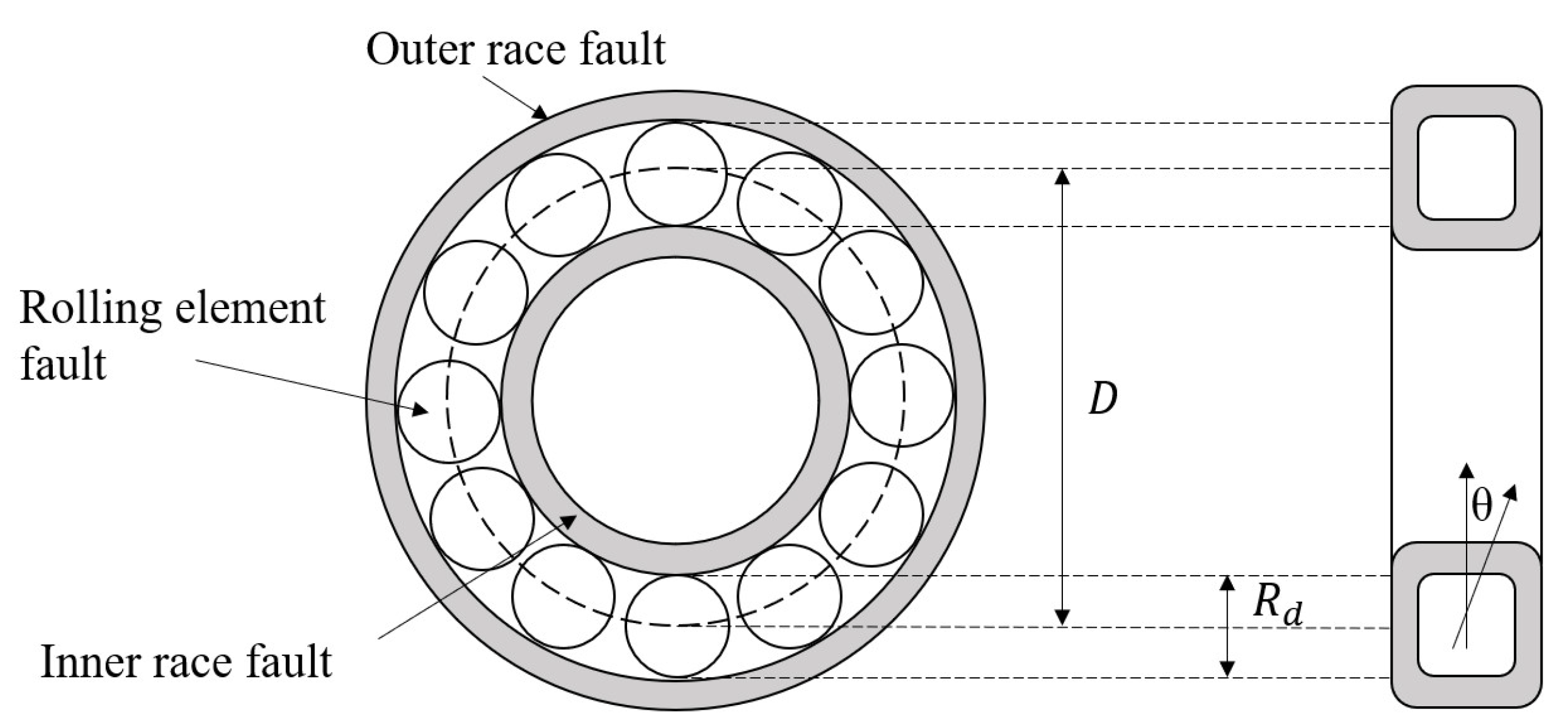
In Equations (1)–(4), is the characteristic frequency of outer ring faults, is the characteristic frequency of rolling element faults, is the characteristic frequency of inner ring faults, and is the characteristic frequency of cage faults. These frequencies depend on the shaft speed (), the number of rolling elements (n), the contact angle with the radial plane (), the roller diameter (), and the pitch diameter (D), as shown in Figure 1.
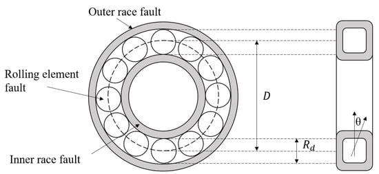
Figure 1.
Schematic Diagram of Possible Failure Locations in a Rolling Bearing.
The radial load has a significant impact on the impact force generated by rolling defects. Every time the rolling element passes through the position of the outer ring defect, the inner ring fault that rotates almost at the speed of the shaft is subjected to different forces. Therefore, all harmonics of are amplitude-modulated by the shaft speed (i.e., ). Similarly, the value of 2 generated by rolling element defects is amplitude-modulated by the cage’s FTF.
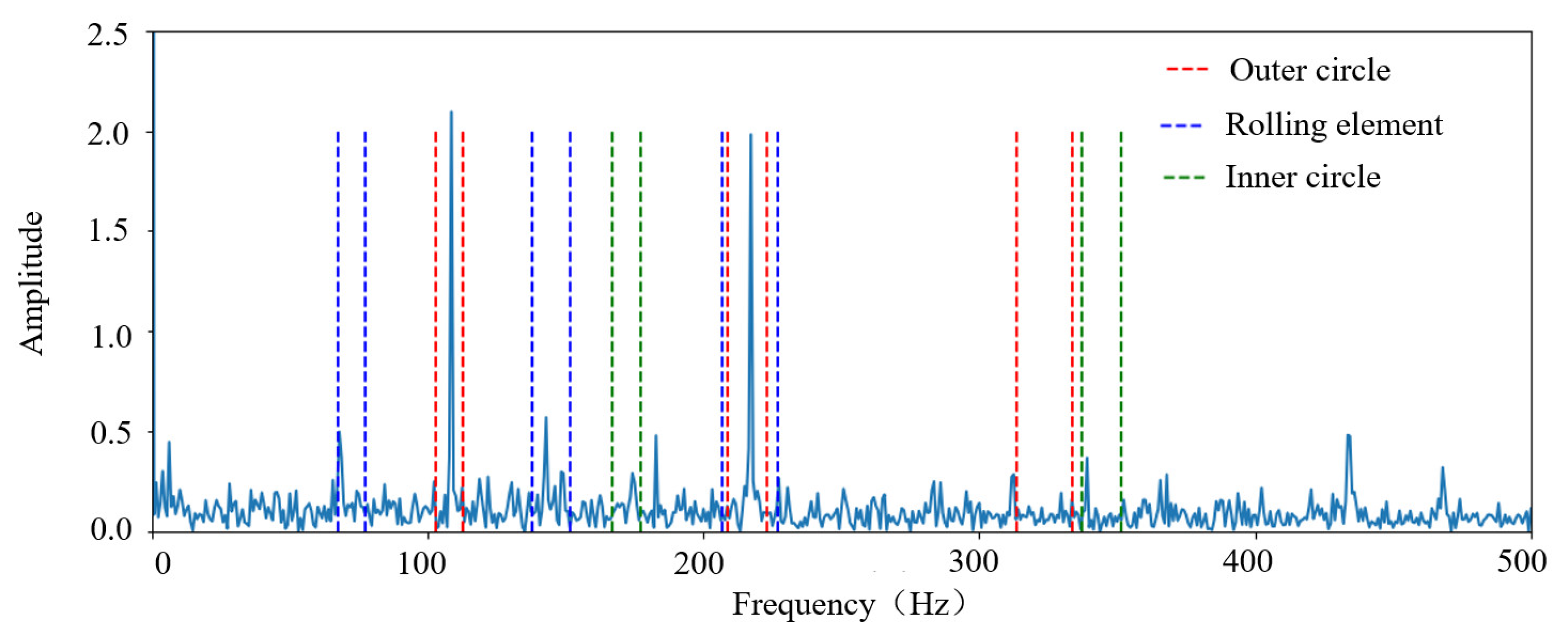
In summary, when a fault occurs inside the bearing, sidebands are generated at intervals of the modulation frequency (i.e., or FTF), centered around or 2. These sidebands are clear symptoms of these bearing defects. Sidebands are typically observed in bearing defect frequencies with random variations of 1–2% of the theoretical fault frequency, the magnitude of the range in this paper is set to . For illustration, take the inner and outer ring fault bearing as an example, Figure 2 shows the EPS-HI calculation process including the value window, where each window of the highest three harmonics of the fault frequency can be seen.
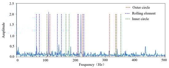
Figure 2.
Schematic diagram of the envelope spectrum and its value window for rolling bearings with inner and outer ring faults.
The fault frequency (including three harmonics) in the envelope spectrum (after DC removal) is utilized to obtain a preliminary health indicator. The entire process comprises two steps. Firstly, based on the previous analysis, a 1.5% value window is defined around the , , and frequency bands. Then, the health indicator EPS-HI is established as a preliminary reference within the constructed value window according to the formula.
The proposed EPS-HI formula is defined as follows:
In Equation (5), n (=3) is the total number of harmonics, h is the order of the harmonic of the fault frequency, ϵ is the value range of the value window at the fault frequency, and defines the root mean square value calculated in the value window of the fault frequency at harmonic h. Similarly, and define the root mean square values of and , respectively. represents the sum of the three largest RMS values among all nine value windows.
When bearings fail, significant changes in amplitude are observed near the harmonics at three different fault frequencies, with the greatest sensitivity occurring during the early fault stages. The numerator in Equation (5) represents the sum of three maximum value windows, allowing the expected health guidance to capture the value window with the largest amplitude change, which is most sensitive.
Compared to the HI established by existing time-frequency statistical parameters (such as root mean square, variance, skewness, and kurtosis), this process takes into account the actual dynamics and mechanical mechanisms when faults occur in the bearings. Therefore, the proposed EPS-HI reflects, to some extent, the actual degradation trend of the bearings. Unlike other methods that focus on a single type of fault, the HI constructed in this paper takes values at all possible fault frequencies and can also reflect the degree of mixed faults to some extent.
2.2. Health Indicator Construction Based on Autoencoder
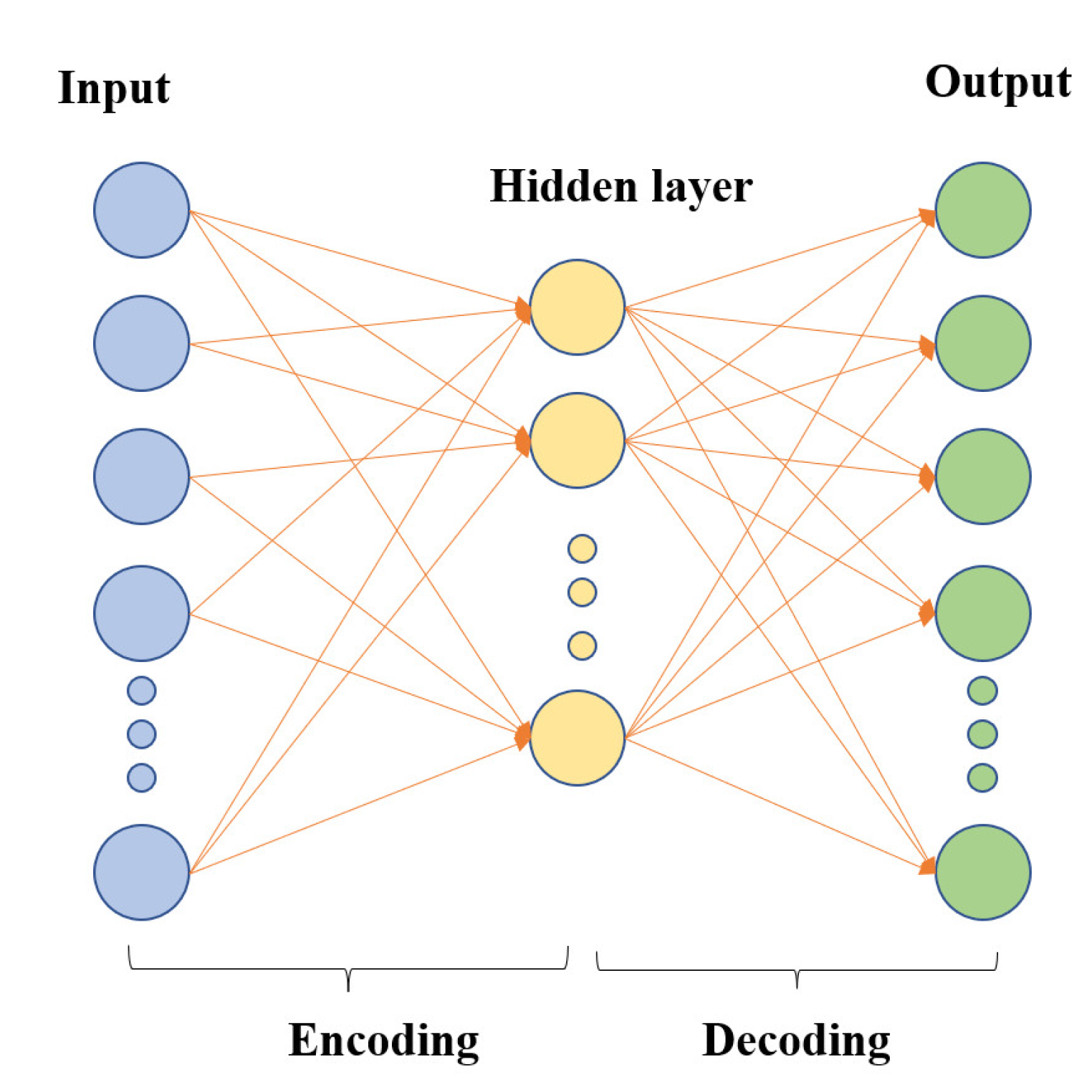
Autoencoders (AE) are an unsupervised learning method consisting of neural networks trained to reconstruct their original inputs, often used for feature dimensionality reduction. Autoencoders have two parts: an encoder and a decoder. The encoder compresses the input signal into a lower-dimensional representation and extracts features. The decoder then takes the encoder output as input and tries to recreate the original input signal. Autoencoders use backpropagation to update internal parameters to minimize errors. The key is constructing a hidden layer with fewer neurons than the input/output layers. Thus, the intermediate hidden layer can produce a feature representation with lower dimensionality than the original data. A typical autoencoder structure is shown in Figure 3.

Figure 3.
Typical autoencoder structure.
Assuming that the encoder input is , where L is the length of the input data. Then, the hidden layer output of the encoder can be expressed as:
where denotes the encoder activation function, and are the weight and bias matrices between adjacent neurons, respectively. On the other hand, the reconstructed output data from the decoder, , is obtained as follows:
where denotes the decoder activation function, and are the decoder weight and bias matrices between adjacent neurons, respectively. The autoencoder weights and bias matrices are optimized by minimizing the following loss function, defined as:
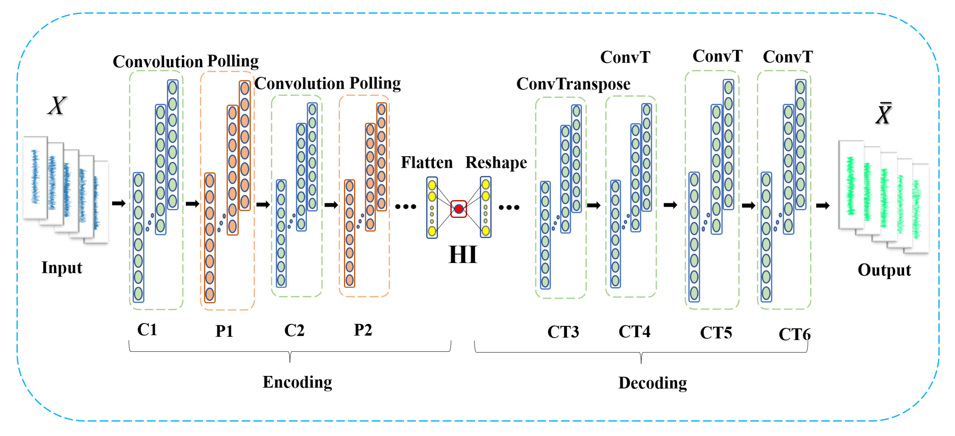
This paper designs a convolutional autoencoder (CAE) structure [26] to generate bearing HI by introducing convolutional operations to replace matrix operations in a basic autoencoder. First, convolution and pooling operations are performed on the input data, referred to as encoding. Then, pooling and convolution reconstruction are performed on the input data, referred to as decoding. The entire network structure expects the input and output data to be as identical as possible. Thus, the output of the intermediate hidden layer can be regarded as a high-level feature extraction of the input data, which is the anticipated HI in this paper. The CAE structure designed in this study is shown in Figure 4.
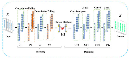
Figure 4.
Convolutional autoencoder structure in this paper.
In this case, choosing to fit based on the EPS-HI obtained in the previous section to train the required autoencoder utilizes the end-to-end feature extraction capability of deep learning and follows the actual degradation trend of bearings. That is, the trained autoencoder has the ability to transform the original vibration data into a health indicator that follows the actual degradation trend. Therefore, obtaining the final health indicator based on EPS-HI through the convolutional autoencoder is a superior result.
The specific steps to obtain the health indicator CAE-EPS-HI through the convolutional autoencoder are as follows:
- (1)
- In the accelerated degradation test of the bearing, the original vibration signal is collected by the accelerometer sensor. Let represent the original vibration signal dataset, where , L represents the length of the vibration sample, and M represents the number of each sample.
- (2)
- In order to obtain a degradation trend based on EPS-HI, the output labels of the encoder during the training process should be (i.e., EPS-HI), which can be represented by Equation (9). It is expected that the encoder’s output is as close to the labels as possible. This part of the loss function can be defined as:
- (3)
- The CAE is trained by the original vibration data and the set labels. By minimizing the loss function, the encoder’s output and the decoder’s output are as close as possible to the labels and the original data . Then, the final loss function can be defined as:
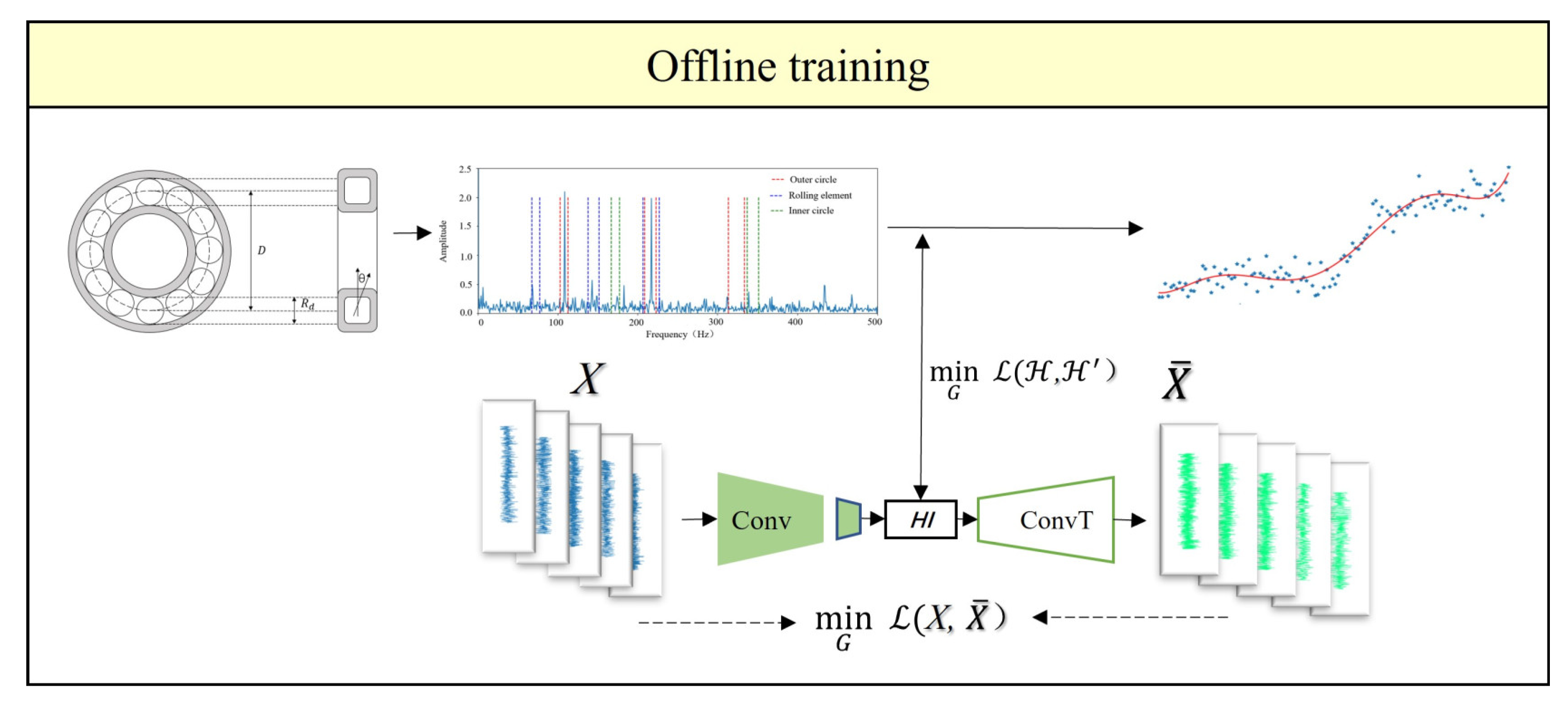
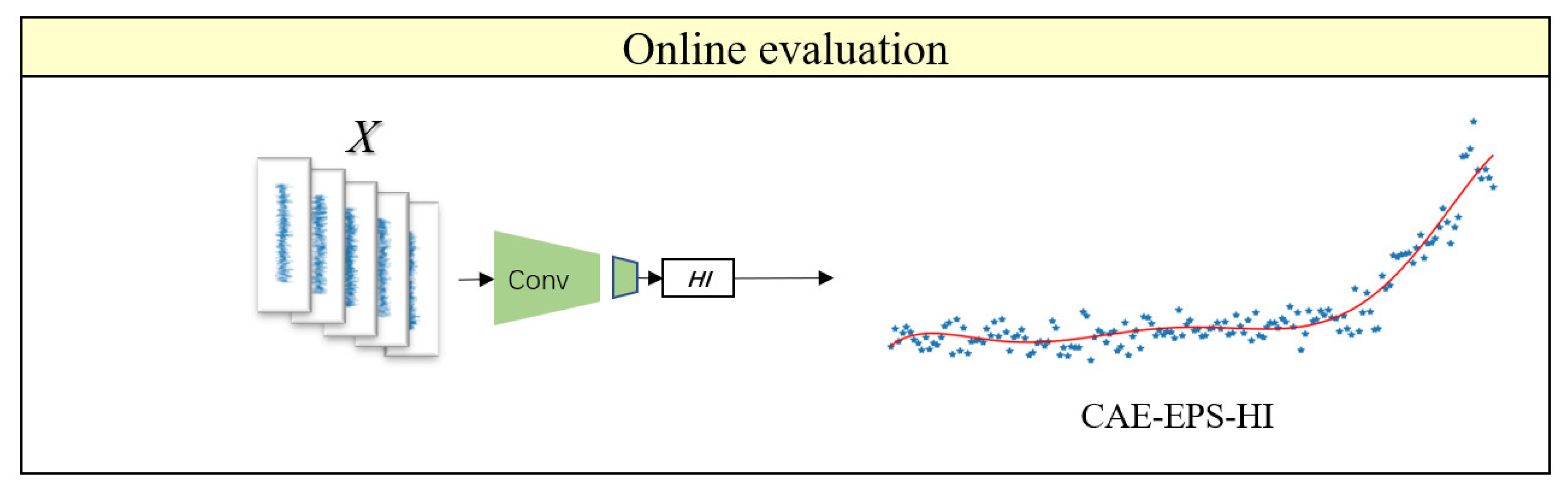
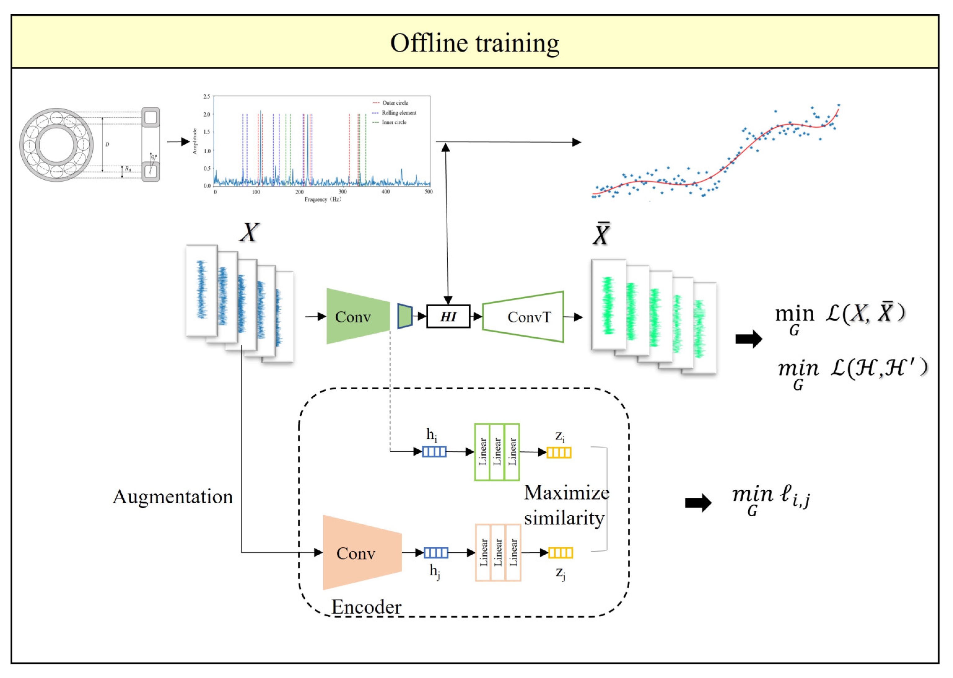
The combined loss function incorporates supervised learning and unsupervised learning methods to train the model, making full use of the degradation information of the bearings to enhance the model’s HI extraction capability. In the offline training phase of the model, the vibration data and labels of the bearings are used for training. The backpropagation algorithm is used to optimize internal parameters to minimize losses, as shown in Figure 5. In the online testing phase of the model, the vibration data of the bearings is used as input, and the trained CAE encoder is utilized to obtain the CAE-EPS-HI, as shown in Figure 6.

Figure 5.
Offline Training Process of CAE.
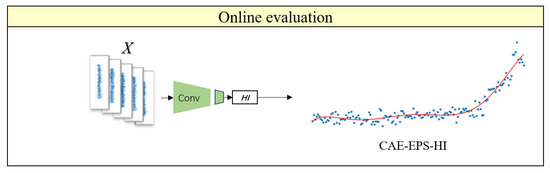
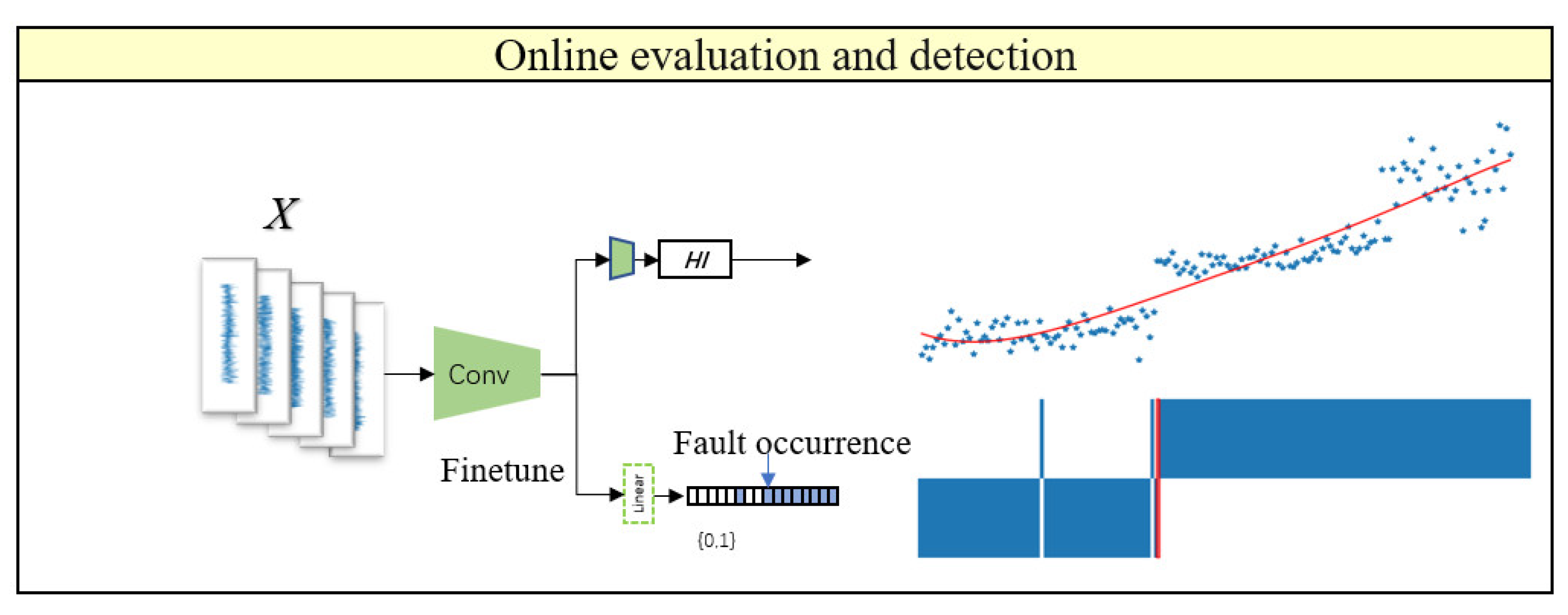
Figure 6.
Online evaluation process of CAE. The blue scatter dots represent the actual output values, and the red lines represent polynomial fitting curves.
After training, the encoder has obtained the capability to transform the original vibration data into a degradation trend that follows the EPS-HI, achieving end-to-end feature extraction and health indicator construction.
In summary, by utilizing the EPS-HI labels obtained in the previous section, training the CAE model with a composite loss function can realize end-to-end HI acquisition and automatic HI extraction. Based on the labels constructed according to the actual mechanical failure mechanisms, utilizing both local and global temporal information can generate more robust and realistic EPS-HI that are closer to actual operating conditions. The trained convolutional autoencoder can automatically extract bearing health indicators (CAE-EPS-HI) from raw vibration signals without requiring expert knowledge, and the extracted HI follows actual degradation trends.
3. Early Fault Detection Method Based on Contrast Learning
3.1. Basic Principle of Contrast Learning
The bearing data typically used may not explicitly provide information about whether early faults have occurred, especially when used online, as early fault states cannot be identified in advance. Alternatively, some labels can be obtained from prior knowledge, specifically indicating that the bearing is healthy at the start of operation and faulty at the end of operation. This serves as a reminder to explore unsupervised learning or self-supervised learning methods. Unsupervised learning can avoid large-scale data annotation due to its ability. Self-supervised learning can be regarded as a representative branch of unsupervised learning. It utilizes the input data itself as supervision to make representations and fine-tune for downstream tasks. The early fault detection framework proposed in this paper can adopt a self-supervised strategy.
For the problem of early fault detection on degradation data from normal operation to failure without state labels, an encoder pretrained with contrast learning (CL) [27] can be utilized to obtain feature representations that demonstrate clear similarities between instances across the entire dataset. This approach ultimately aims to enhance the deep feature extraction capabilities of a self-encoder, enabling high discrimination. Based on these highly discriminative representations, by fine-tuning a downstream classification model with proper task settings, the fault occurrence time (FOT) can be readily determined to easily evaluate the bearing state.
Our goal is to train an encoder without annotated supervision. A good feature extractor should map more similar samples closer in the feature space, with the similarity measured in the space as:
where is a deep neural network representing the parameters as the encoder, mapping instances x to features h.
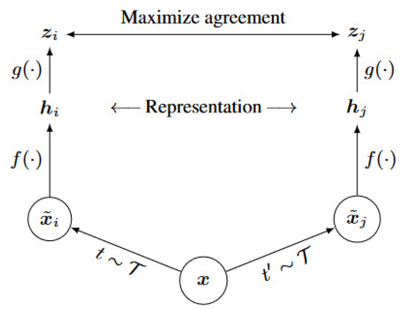
SimCLR [28]: a simple framework for contrast learning of visual representations is illustrated in Figure 7.
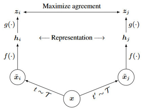
Figure 7.
The Framework of Contrast Learning.
Our framework allows for various choices of network architectures without any restrictions. The CAE encoder from the previous section, denoted as f(·), is chosen. It takes the augmented data as input and produces two feature vectors h as output.
where is the output of the pooling layer, denotes the data augmented. The obtained h is then passed through an MLP (i.e., fully connected network) and projected by the operation to obtain .
In this framework, is used for calculating the contrastive loss. However, the ultimate representation desired is . The expected feature extractor is (the encoding part of the CAE encoder in this paper). For downstream tasks, the MLP used during training needs to be discarded (previous studies have shown that the obtained by calculating the loss through during training leads to better results, and the MLP only serves as an auxiliary for the training process).
Next, the loss function for the contrast learning network is defined as follows. Given a dataset containing a pair of positive instances and , N samples are randomly sampled, and from the extended samples of the mini-batch, 2N augmented data points are obtained. Negative examples are not explicitly sampled. For the given original data, two augmentations and are defined as positive examples, while the other 2(N − 1) extended samples are considered negative examples. In this way, during the learning process, the model will pull closer to the distance between positive examples while pushing away negative examples, enabling it to learn the similarities between objects to some extent. The NT-Xent (Normalized Temperature-Tuned Cross-Entropy Loss) loss function is adopted, as defined in Equation (14).
where represents the dot product (i.e., cosine similarity) between and after normalization, equals 1 only when and equals 0 otherwise, is the temperature parameter, which can appropriately scale the computation of similarity so that the similarity is not limited to [−1,1]. represents the feature vector of positive examples in the representation space.
In the numerator part of the loss function, the closer the distance between the two positive examples, the smaller the loss function, which means the closer the distance between positive examples, the better. The denominator part indicates that the farther the distance between positive and negative examples, the smaller the loss function, and the farther the distance, the smaller the loss function. By defining the loss function, it guides the direction of model training to make the model closer and closer to the expected target.
3.2. Early Fault Detection Based on Contrast Learning
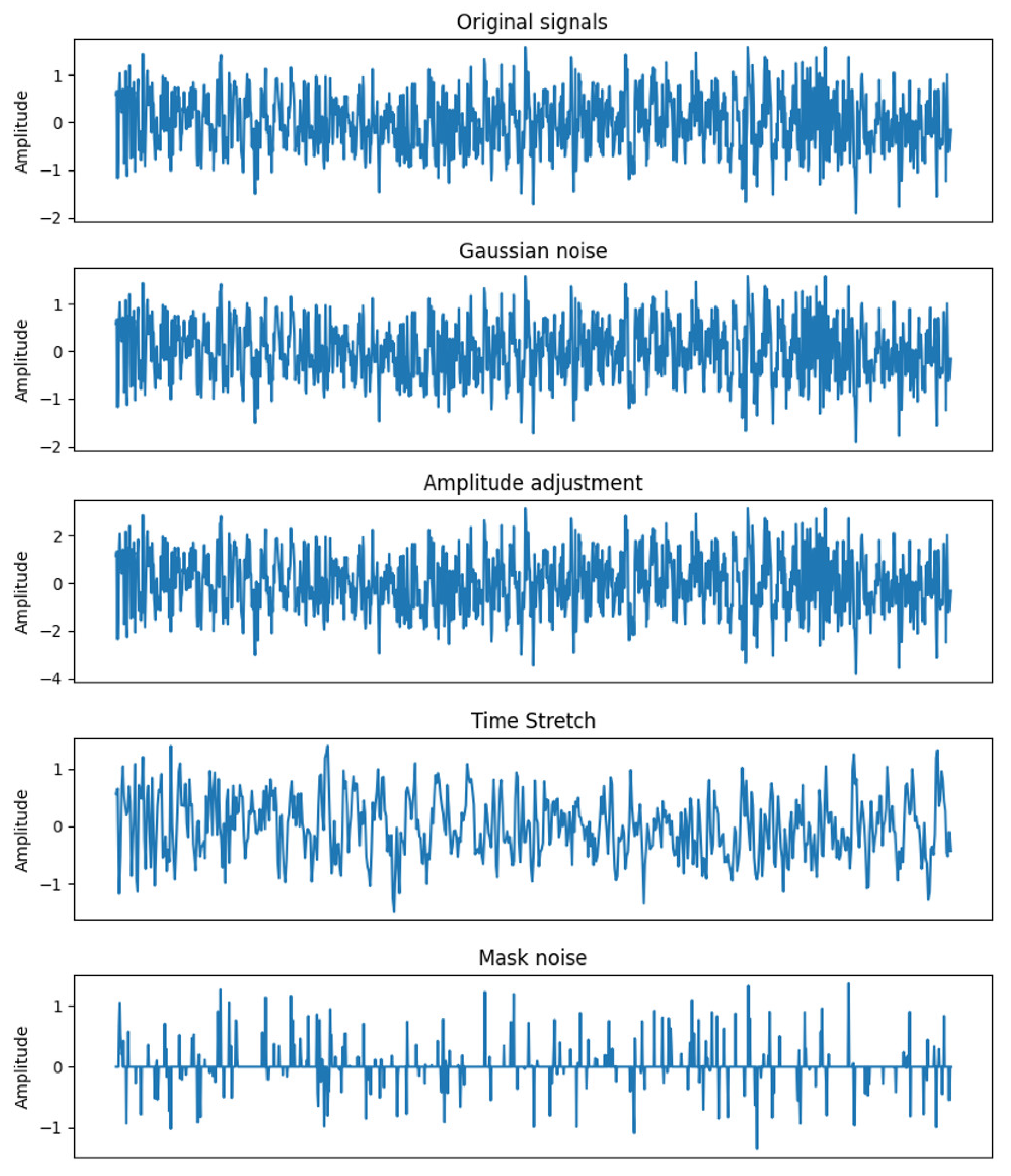
Contrast learning is commonly used in the field of images. This article requires the use of corresponding data augmentation methods when applied to time-series data. For given data, data augmentation is carried out in the following ways: a segment of vibration data are selected for augmentation, as shown in Figure 8.
- (1)
- Gaussian noise: Gaussian noise is a data augmentation method that intuitively applies to one-dimensional signals. It is carried out by adding a random sequence G:
- (2)
- Amplitude adjustment: The amplitude of the signal sequence is adjusted by a factor of s:
- (3)
- Time stretching: The signal length is stretched to times of the original length through downsampling or upsampling interpolation, where represents the stretching coefficient. Then, zero padding or truncation is applied to recover the signal length.
- (4)
- Mask noise: Given a mask M of length N, where the probability of each element being 0 is , otherwise 1. Then, mask the signal:
In the second stage of this section, the parameters of the feature extraction layer (autoencoder) trained in the first stage are loaded and frozen, and supervised learning is performed with a small amount of labeled samples (only training the fully connected layer). The bearings were healthy at the start of the run and faulty at the end of the run. This small portion of data is used to train the fully connected layer Linear [192,1]. The loss function for this stage is the cross-entropy loss function, CrossEntropyLoss(). The epoch for network training is set to 300, and convergence is achieved when the training loss term reaches its minimum. The learning rate in this study is set to 0.001, with a learning rate reduction strategy implemented. If the loss does not decrease continuously for 50 iterations, the learning rate is reduced to 0.1 times the original value, with a minimum value of 0.0001. The Adam optimizer is utilized for optimization.

Figure 8.
Schematic Diagrams of Data Augmentation.
Figure 8.
Schematic Diagrams of Data Augmentation.
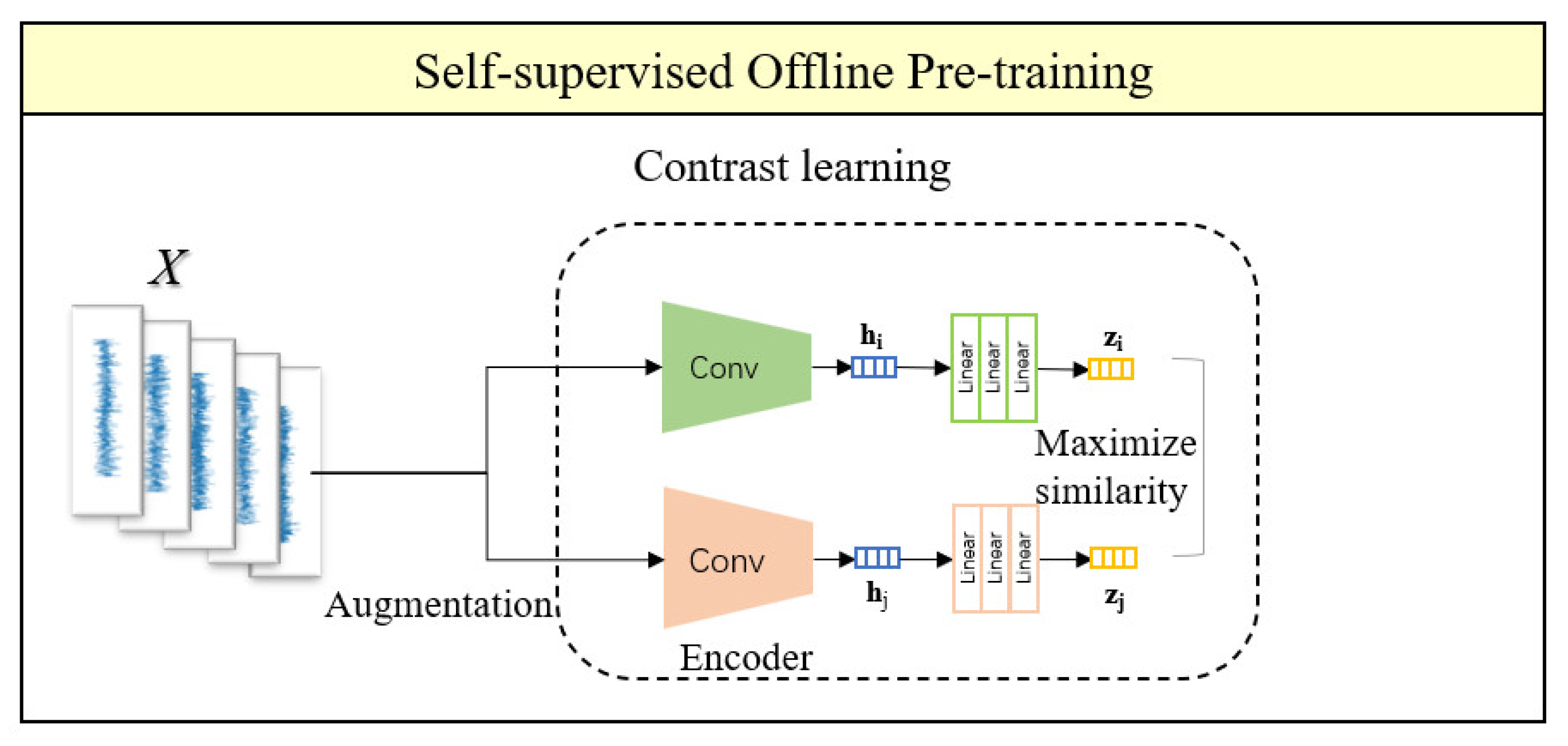
As shown in Figure 9, the model structure consists of an upper and lower branch for the self-supervised offline pre-training framework. The main purpose is to minimize the distance between two positive examples and maximize the distance between positive and negative examples. This allows the model to learn to discriminate between similar instances by ignoring some features, so that the pre-trained model can demonstrate stronger discrimination ability in downstream tasks.
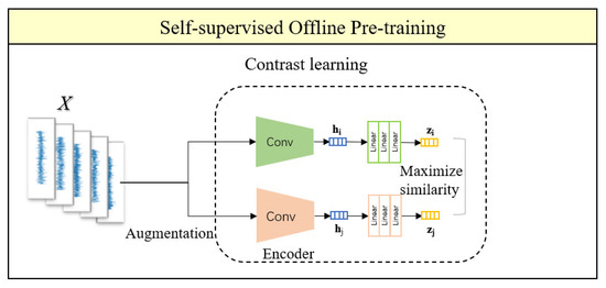
Figure 9.
Diagram of self-supervised offline pre-training framework.
In the online detection part, by referring to the knowledge of fine-tuning in transfer learning, the trained encoder is transferred to the downstream task and connected to the linear layer. The linear layer output is controlled to be 0 or 1, where 0 represents normal and 1 represents fault, thus setting up the fault detection task as a binary classification problem of normal (N) vs. fault (F). In the training dataset, 10% of the samples from the beginning stage and 5% of the samples from the end stage of the bearing lifecycle data are selected for health and failure labeling, respectively. This small amount of data is then used to train the fully connected layer. In this section, only a small amount of annotated data is required, and the annotation process is simple, significantly reducing the workload of annotating data. The online monitoring workflow is illustrated in Figure 10.
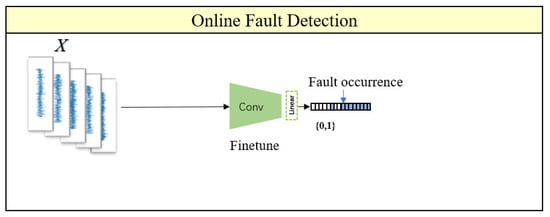
Figure 10.
Diagram of online monitoring workflow.
By leveraging a large amount of unlabeled data and using contrast learning as guidance, an encoder model with strong discrimination ability and its corresponding feature representations are learned. The goal of contrast learning is to group similar samples together while separating different samples far apart. For the input data, the encoder is able to extract key information while ignoring irrelevant information. It is hoped that the pre-trained model can have certain transfer learning effects on downstream tasks to enhance generalization ability.
4. Health Assessment and Fault Detection Neural Network (ADNN)
In Part 2 and Part 3, an encoder structure is used. By integrating the encoder for health condition assessment from Part 1 (which obtains health indicators), the two encoders can be organically combined to obtain the health assessment and early fault detection neural network (ADNN), as shown in Figure 11.
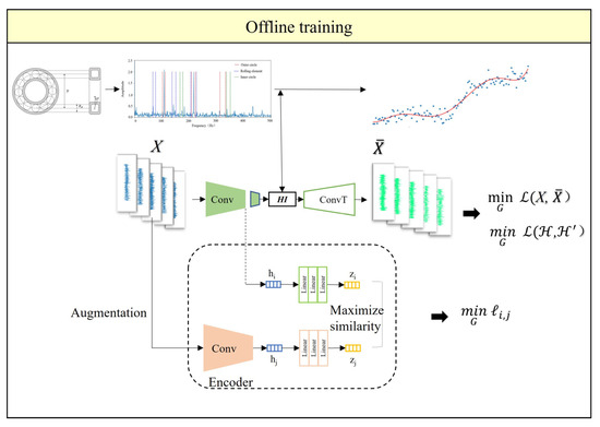
Figure 11.
Online training process of the integrated network for health assessment and early fault detection.
The loss function for the integrated network is defined as:
For the fault detection part of this integrated network, the encoder takes in raw data as input without data augmentation, which differs from the traditional contrast learning training approach.
By utilizing transfer learning methods to fine-tune the pretrained encoder (with strong feature extraction and discrimination capabilities) for downstream tasks, online health assessment can obtain health indicators, and online detection can obtain fault occurrence points, thus starting the prediction phase. The online processes of health assessment and fault monitoring are illustrated in Figure 12.

Figure 12.
Integrated Network for Health Assessment and Early Fault Detection. The blue scatter dots represent the actual output values, and the red lines represent polynomial fitting curves.
The innovations of Section 2 and Section 3 in this paper are: proposing a method of constructing health indicators based on bearing fault mechanisms, integrating contrast learning, transfer learning and metric learning ideas, training an encoder with strong feature extraction and discrimination capabilities, and skillfully integrating the evaluation and detection parts of the model to obtain an integrated training network, with a small-sized model that can solve online evaluation and detection problems.
5. Experiments
For the RUL estimation of rolling bearing driven by experimental data, the rolling bearing experimental data from operation to failure adopted in this paper comes from the XJTU-SY [29] bearing data center, and its bearing degradation experiment platform is shown in Figure 13. The experimental bearing is the UER204 rolling bearing produced by LDK. Two acceleration sensors were installed on the test bearing, with a sampling rate of 25.6 kHz and a sampling interval of 1 min. To reduce model size and computation, each sample of 1.28 s duration is divided into several samples of 1280 ms duration. Signals under three different operating conditions were collected for experimental research, as shown in Table 1.
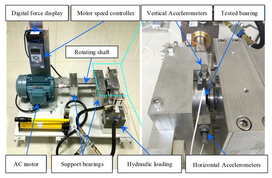
Figure 13.
XJTU-SY bearing degradation experiment platform.

Table 1.
Description of the XJTU-SY Dataset.
All case studies in this paper were conducted on a Windows 10 platform using Python 3.9 and PyTorch 1.9, with the following configuration: i7 8700K, NVIDIA 1070Ti, 32 GB RAM.
5.1. Implementation Details
As shown in Figure 4, the CAE encoder consists of three layers of 1D convolutional layers (C1 to C3) and three layers of 1D max pooling layers (P1 to P3). The output of the encoder is the HI, which also serves as the input to the decoder. The decoder consists of six layers of 1D transposed convolutional layers. Ultimately, the input and output data are expected to be consistent. The activation function uses Sigmoid for all layers. The Adam optimizer is adopted, and the loss function is calculated using mean square error loss (MSELoss). Batch normalization (BatchNorm) is performed after each layer, with a batch size of 64. The input data dimension is [−1, 1, 1280]. Specific model parameters are shown in Table 2 and Table 3.
Table 2.
Encoder layer parameters.
Table 3.
Decoder layer parameters.
To integrate with the previous health assessment section, the encoder part in the diagram shares the same structure as the first five layers of the encoder in the previous section (i.e., with the same three convolutional layers C1, C2, C3, and two pooling layers P1, P2). The batch size is 64, and Adam optimizer is used with a learning rate of 0.001. The specific parameters are shown in Table 4.
Table 4.
Parameters of layers in the fault detection encoder.
The feature representation extracted from the encoder can be used for downstream tasks. It is then passed through three linear layers to obtain , which is used to calculate the contrastive loss. The specific parameters of the linear layers are shown in Table 5.
Table 5.
Parameters of linear layers in fault detection.
5.2. Health Indicators Comparison
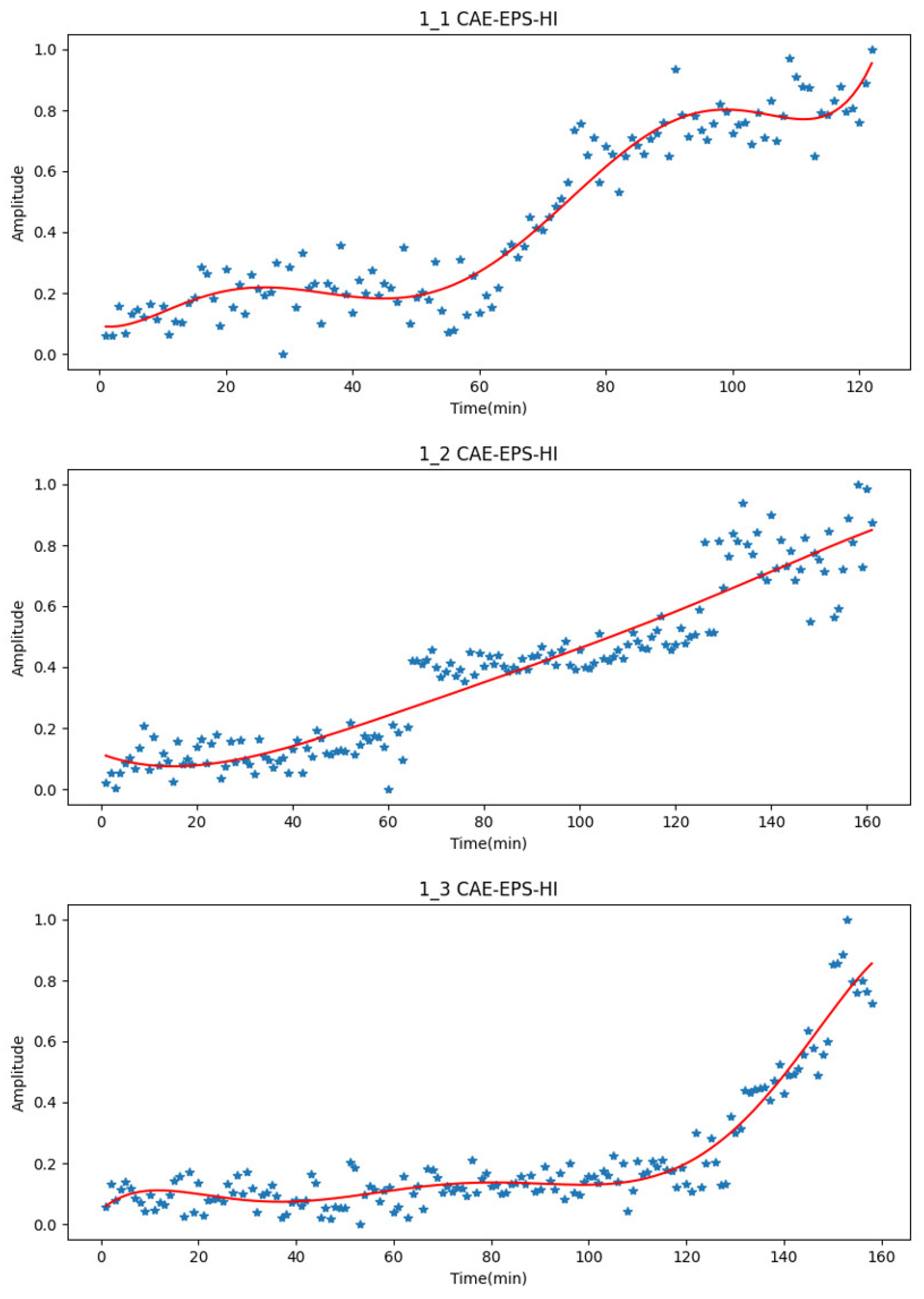
Taking Bearing1_1, Bearing1_2, and Bearing1_3 as examples, the comparison between the EPS-HI obtained through the value window of Equation (5) and the CAE-EPS-HI obtained by the encoder is shown in Figure 14. In the figure, the actual values are represented by the blue scatter points, while the red curve represents the fitted values for ease of display.
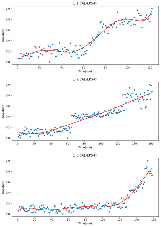
Figure 14.
CAE-EPS-HI (test set results) for faulty bearings. The blue scatter dots represent the actual output values, and the red lines represent polynomial fitting curves.
After the health guidelines CAE-EPS-HI are obtained, a degradation trend can be clearly observed. Significant jumps in the health guidelines will be observed during the early stages of failure.
Several traditional methods will be introduced and compared with the proposed CAE-EPS-HI. The root mean square (RMS) of the original vibration signal is a classic bearing health indicator, which is directly used to represent the health status of bearings. Traditional Convolutional Neural Networks (CNN) can also obtain health indicators after setting the parameters of each network layer.
There are significant differences in the degradation trends of bearings reflected by different features. Some features are insensitive to bearing degradation information, have high volatility, and do not experience significant sudden changes in early faults. Therefore, some evaluation indicators need to be compared and analyzed. The construction of HI for bearings is to facilitate subsequent RUL prediction of remaining service life, and it is also necessary to compare the trend and robustness of HI. To assess the performance of different types of HI, their monotonicity, correlation, and robustness were calculated. The details of the three measurement methods can be found in the relevant section [30].
A good bearing health guide should have a certain degree of monotony to avoid the phenomenon of “health improvement” at the data level. is defined as:
where is the number of monotonically upward vectors between a certain feature point and the next point, and is the total length of HI. is used to measure the increasing or decreasing trend of HI. When = 1, it indicates that HI is completely monotonic, with values limited to the range of 0 to 1, and is positively correlated with health guidance performance.
The health guidelines constructed based on the full life cycle data of bearings should be correlated with time. This article uses the Spearman correlation coefficient to describe the correlation between health guidance and time. is calculated as follows:
where is the total length of HI and is the rank difference of the time series after updating the order arrangement. Tre is used to measure the linear correlation between HI and time, with a numerical limit between 0 and 1. The magnitude of the value is positively correlated with the correlation between HI.
The robustness of a health indicator refers to the ability to distinguish the various stages of degradation well, with strong stage separability, which helps indirectly improve the diagnostic ability of the model. is defined as:
where is the total number of observations, is the smoothed average trend, and is the fluctuation term. Each feature parameter should undergo the same smoothing process during the comparison of robustness indicators.
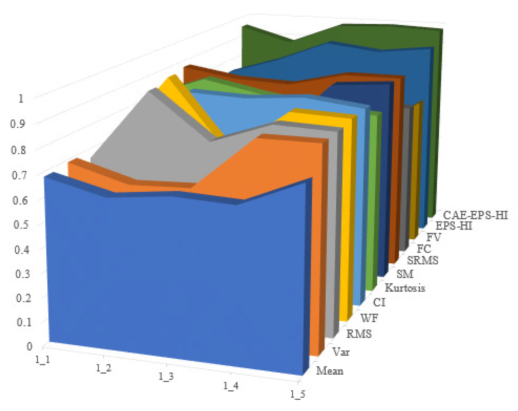
Operating conditions 2 and 3 in the XJTU dataset are utilized as the training set, while operating condition 1 serves as the testing set. The process is repeated ten times to obtain evaluation results for each test and calculate their average values. Time-domain features such as mean, variance, root mean square, waveform factor, clearance indicator, and kurtosis are selected, along with frequency-domain features including spectral mean, spectrum root mean square, frequency centroid, and frequency variance. A comparison between EPS-HI and CAE-EPS-HI is conducted in this study, with all features normalized during evaluation calculations. The experimental results are shown in Figure 15, Figure 16 and Figure 17.
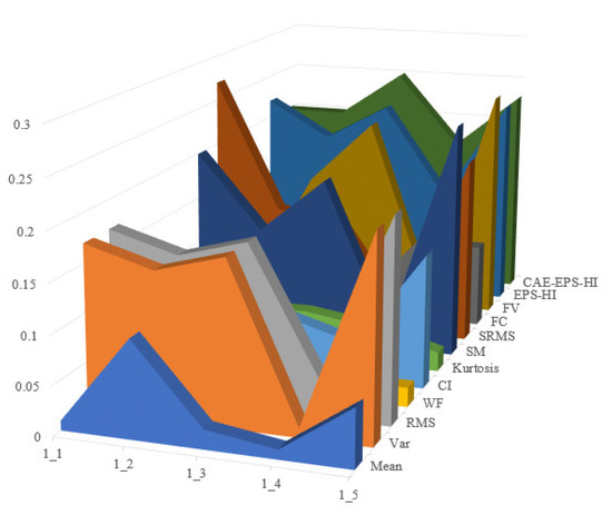
Figure 15.
Comparison of experimental results based on monotonicity.
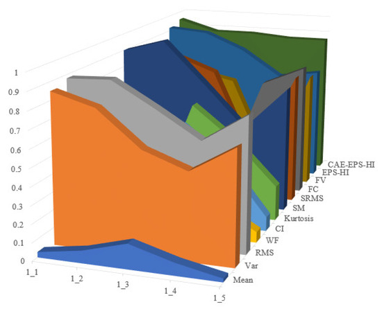
Figure 16.
Comparison of experimental results based on correlation.
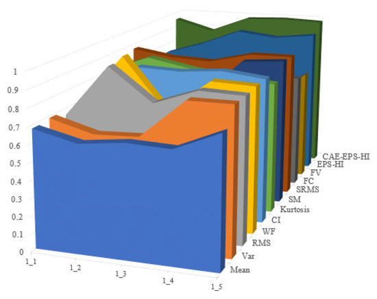
Figure 17.
Comparison of experimental results based on robustness.
It is not difficult to see that the health guideline CAE-EPS-HI proposed in this article has good performance in monotonicity, correlation, and robustness. In each evaluation indicator, the last layer of the dark green trend wall can be clearly seen, indicating that the effect in the dataset is better than the other HI mentioned.
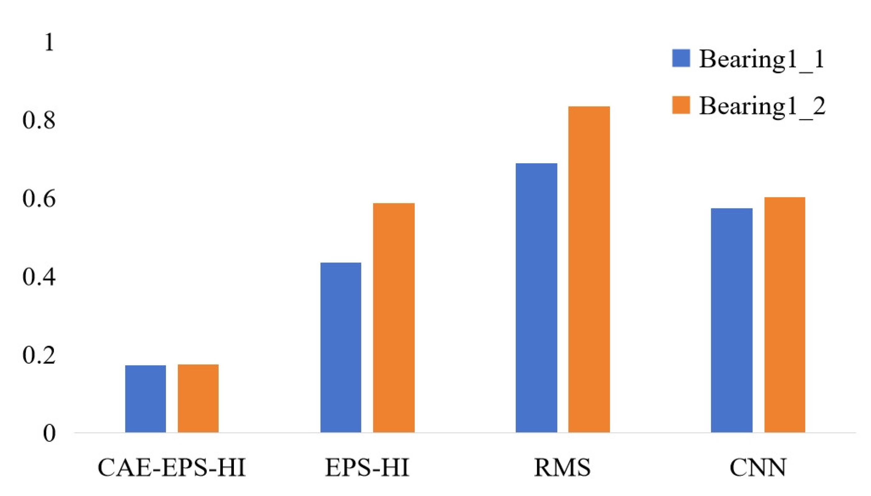
The Mean Absolute Error (MAE) between the smoothed computed HI and the actual HI was calculated as a metric. The MAE values are depicted in Figure 18. The proposed CAE-EPS-HI outperforms the other HI in both respects.
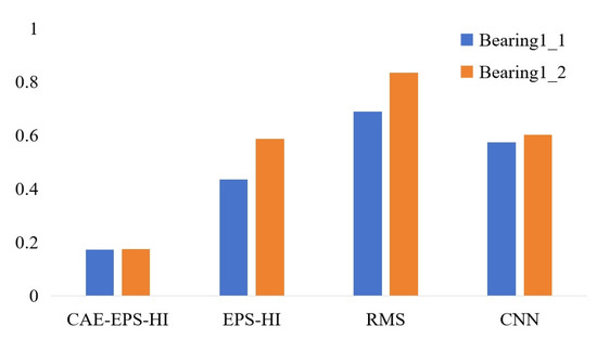
Figure 18.
MAE of the 4 kinds of HI of bearing1_1 and bearing1_2.
In summary, from the perspectives of monotonicity, correlation, robustness, and MAE values, this method clearly outperforms the other methods in experimental effectiveness.
Furthermore, the fact that CAE-EPS-HI performs better than EPS-HI suggests that the training through encoding, decoding, and contrastive learning within the composite network enhances the model’s feature extraction capabilities and discriminative power. As a result, the obtained CAE-EPS-HI demonstrates slightly better predictive performance.
5.3. Fault Detection Results
After pre-training, the model can easily be transferred to downstream tasks. In the complete life cycle data of bearings, only the initial normal data and the data at the end when the bearing fails are readily obtainable. The linear layer of the network is trained using the two parts of limited data, labeled as normal and fault. The model parameters of the encoder are kept fixed, and the output of the linear layer is controlled to be either 0 or 1. A time-evolving state sequence is obtained, with each element being 0 or 1, representing normal (N) and fault (F), respectively.
During online detection, false alarms are inevitable due to interference from other factors in data collection. These inevitable interference factors that make the model produce misjudgments in healthy conditions, causing false alarms. As long as there is continuous data input, the false alarm rate will be greatly reduced. In consideration of the above reasons, a reference coefficient [27] is set, that is, if the alarm persists within 0.2% of the number of input samples and the subsequent data remains normal, it is considered a false alarm. Therefore, the threshold of is selected to predict early-stage faults as soon as possible while also minimizing the occurrence of false alarms, thereby enhancing the reliability of the predictions.
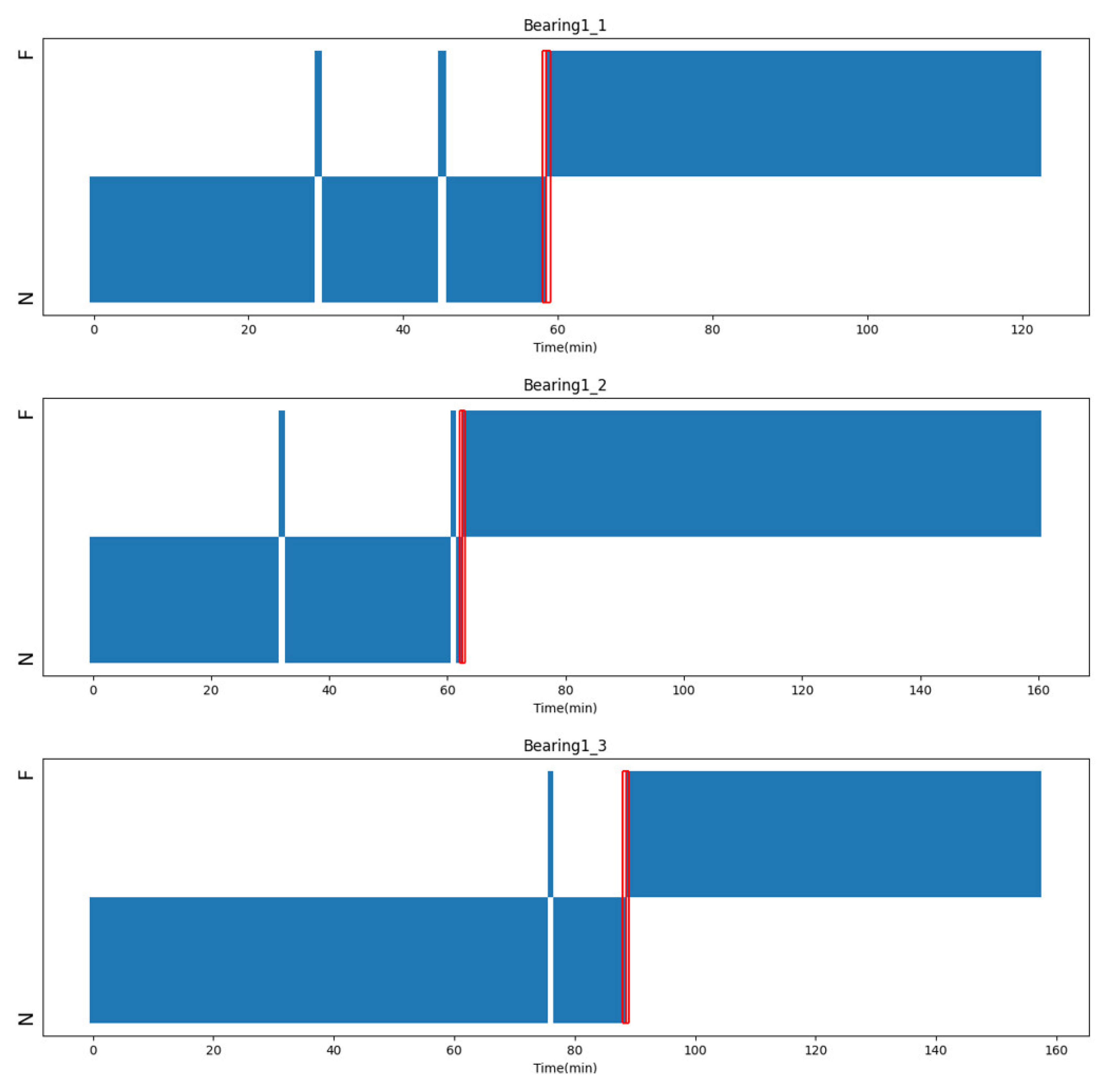
Operating conditions 2 and 3 in the XJTU dataset are utilized as the training set, while operating condition 1 serves as the testing set. Based on the aforementioned setup, the occurrence of faults for each bearing is predicted online. Taking the bearings Bearing1_1, 1_2, and 1_3 as examples and the vibration data as input, the detection results are as shown in Figure 19. The red dashed line represents the moment of fault occurrence, and the regions N and F, respectively, represent the normal and fault states of the bearings. The experimental results indicate that our proposed method achieves early fault detection across all tested bearings.
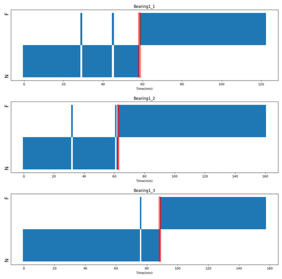
Figure 19.
Early fault detection results of bearing1_1, bearing1_2 and bearing1_3. The early occurrence points of fault are represented by the red boxes in the picture.
6. Conclusions
Through the training of autoencoders and contrastive learning, the model has strong feature extraction capabilities. The established health indicator can reflect the actual degradation level of bearings to a certain extent. The pre-trained autoencoder can be easily transferred to similar downstream tasks. It only requires quick fine-tuning without the need to train from scratch, making the method highly referential. The online detection network does not depend on any data processing or statistical features; it directly inputs the original vibration data to realize an end-to-end construction of health indicators and early fault detection.
In addition, the following shortcomings and prospects have been identified:
In the fault detection phase, further definition of early fault characteristics is needed, along with the identification of suitable evaluation criteria to differentiate between premature and late warnings. Building on the ADNN, further exploration of methods to reduce the dependency on prior knowledge and annotations is warranted.
Author Contributions
Conceptualization, D.W., D.C. and G.Y.; methodology, D.W.; software, D.W.; validation, D.W., D.C. and G.Y.; investigation, D.W.; resources, G.Y.; data curation, D.W. and D.C.; writing—original draft preparation, D.W.; writing—review and editing, D.W., D.C. and G.Y.; visualization, D.W. and D.C.; supervision, G.Y.; project administration, G.Y. All authors have read and agreed to the published version of the manuscript.
Funding
This research received no external funding.
Data Availability Statement
The original data presented in the study are openly available in Ref. [30].
Acknowledgments
The authors would like to thank XJTU-SY for the open-source bearing data for the experiments in this work.
Conflicts of Interest
The authors declare no conflicts of interests.
References
- Wang, D.; Tsui, K.L.; Miao, Q. Prognostics and health management: A review of vibration based bearing and gear health indicators. IEEE Access 2017, 6, 665–676. [Google Scholar] [CrossRef]
- Gupta, P.; Pradhan, M.K. Fault detection analysis in rolling element bearing: A review. Mater. Today Proc. 2017, 4, 2085–2094. [Google Scholar] [CrossRef]
- Brusa, E.; Bruzzone, F.; Delprete, C. Health indicators construction for damage level assessment in bearing diagnostics: A proposal of an energetic approach based on envelope analysis. Appl. Sci. 2020, 10, 8131. [Google Scholar] [CrossRef]
- Duong, B.P.; Khan, S.A.; Shon, D. A reliable health indicator for fault prognosis of bearings. Sensors 2018, 18, 3740. [Google Scholar] [CrossRef] [PubMed]
- Soualhi, M.; Nguyen, K.T.P.; Soualhi, A. Health monitoring of bearing and gear faults by using a new health indicator extracted from current signals. Measurement 2019, 141, 37–51. [Google Scholar] [CrossRef]
- Guo, L.; Li, N.; Jia, F. A recurrent neural network based health indicator for remaining useful life prediction of bearings. Neurocomputing 2017, 240, 98–109. [Google Scholar] [CrossRef]
- Kumar, A.; Parkash, C.; Vashishtha, G. State-space modeling and novel entropy-based health indicator for dynamic degradation monitoring of rolling element bearing. Reliab. Eng. Syst. Saf. 2022, 221, 108356. [Google Scholar] [CrossRef]
- Chen, X.; Shen, Z.; He, Z. Remaining life prognostics of rolling bearing based on relative features and multivariable support vector machine. Proc. Inst. Mech. Eng. Part C J. Mech. Eng. Sci. 2013, 227, 2849–2860. [Google Scholar] [CrossRef]
- Yang, C.; Ma, J.; Wang, X. A novel based-performance degradation indicator RUL prediction model and its application in rolling bearing. ISA Trans. 2022, 121, 349–364. [Google Scholar] [CrossRef]
- Ding, P.; Jia, M.; Ding, Y. Intelligent machinery health prognostics under variable operation conditions with limited and variable-length data. Adv. Eng. Inform. 2022, 53, 101691. [Google Scholar] [CrossRef]
- Xu, W.; Jiang, Q.; Shen, Y. RUL prediction for rolling bearings based on Convolutional Autoencoder and status degradation model. Appl. Soft Comput. 2022, 130, 109686. [Google Scholar] [CrossRef]
- Chen, D.; Qin, Y.; Wang, Y. Health indicator construction by quadratic function-based deep convolutional auto-encoder and its application into bearing RUL prediction. ISA Trans. 2021, 114, 44–56. [Google Scholar] [CrossRef] [PubMed]
- Islam, M.M.M.; Prosvirin, A.E.; Kim, J.M. Data-driven prognostic scheme for rolling-element bearings using a new health index and variants of least-square support vector machines. Mech. Syst. Signal Process. 2021, 160, 107853. [Google Scholar] [CrossRef]
- Meng, J.; Yan, C.; Chen, G. Health indicator of bearing constructed by rms-CUMSUM and GRRMD-CUMSUM with multifeatures of envelope spectrum. IEEE Trans. Instrum. Meas. 2021, 70, 1–16. [Google Scholar] [CrossRef]
- Ni, Q.; Ji, J.C.; Feng, K. Data-driven prognostic scheme for bearings based on a novel health indicator and gated recurrent unit network. IEEE Trans. Ind. Inform. 2022, 19, 1301–1311. [Google Scholar] [CrossRef]
- Yan, T.; Wang, D.; Xia, T. A generic framework for degradation modeling based on fusion of spectrum amplitudes. IEEE Trans. Autom. Sci. Eng. 2020, 19, 308–319. [Google Scholar] [CrossRef]
- Mao, W.; Ding, L.; Liu, Y. A new deep domain adaptation method with joint adversarial training for online detection of bearing early fault. ISA Trans. 2022, 122, 444–458. [Google Scholar] [CrossRef] [PubMed]
- Brkovic, A.; Gajic, D.; Gligorijevic, J. Early fault detection and diagnosis in bearings for more efficient operation of rotating machinery. Energy 2017, 136, 63–71. [Google Scholar] [CrossRef]
- Lu, W.; Li, Y.; Cheng, Y. Early fault detection approach with deep architectures. IEEE Trans. Instrum. Meas. 2018, 67, 1679–1689. [Google Scholar] [CrossRef]
- Xie, F.; Li, G.; Song, C. The Early Diagnosis of Rolling Bearings’ Faults Using Fractional Fourier Transform Information Fusion and a Lightweight Neural Network. Fractal Fract. 2023, 7, 875. [Google Scholar] [CrossRef]
- Xu, M.; Zheng, C.; Sun, K. Stochastic resonance with parameter estimation for enhancing unknown compound fault detection of bearings. Sensors 2023, 23, 3860. [Google Scholar] [CrossRef] [PubMed]
- Tang, H.; Tang, Y.; Su, Y. Feature extraction of multi-sensors for early bearing fault diagnosis using deep learning based on minimum unscented kalman filter. Eng. Appl. Artif. Intell. 2024, 127, 107138. [Google Scholar] [CrossRef]
- Yan, J.; Liu, Y.; Ren, X. An Early Fault Detection Method for Wind Turbine Main Bearings Based on Self-Attention GRU Network and Binary Segmentation Changepoint Detection Algorithm. Energies 2023, 16, 4123. [Google Scholar] [CrossRef]
- Nguyen, H.N.; Kim, J.; Kim, J.M. Optimal sub-band analysis based on the envelope power spectrum for effective fault detection in bearing under variable, low speeds. Sensors 2018, 18, 1389. [Google Scholar] [CrossRef] [PubMed]
- Zhang, B.; Miao, Y.; Lin, J. Weighted envelope spectrum based on the spectral coherence for bearing diagnosis. ISA Trans. 2022, 123, 398–412. [Google Scholar] [CrossRef] [PubMed]
- Cheng, Z.; Sun, H.; Takeuchi, M. Deep Convolutional Autoencoder-Based Lossy Image Compression. In Proceedings of the 2018 Picture Coding Symposium (PCS), San Francisco, CA, USA, 24–27 June 2018. [Google Scholar]
- Ding, Y.; Zhuang, J.; Ding, P. Self-supervised pretraining via contrast learning for intelligent incipient fault detection of bearings. Reliab. Eng. Syst. Saf. 2022, 218, 108126. [Google Scholar] [CrossRef]
- Chen, T.; Kornblith, S.; Norouzi, M. A Simple Framework for Contrastive Learning of Visual Representations. In Proceedings of the International Conference on Machine Learning (ICML), Vienna, Austria (Virtual), 13–18 July 2020. [Google Scholar]
- Wang, B.; Lei, Y.; Li, N.; Li, N. A Hybrid Prognostics Approach for Estimating Remaining Useful Life of Rolling Element Bearings. IEEE Trans. Reliab. 2018, 69, 401–412. [Google Scholar] [CrossRef]
- Zhang, B.; Zhang, L.; Xu, J. Degradation feature selection for remaining useful life prediction of rolling element bearings. Qual. Reliab. Eng. Int. 2016, 32, 547–554. [Google Scholar] [CrossRef]


Disclaimer/Publisher’s Note: The statements, opinions and data contained in all publications are solely those of the individual author(s) and contributor(s) and not of MDPI and/or the editor(s). MDPI and/or the editor(s) disclaim responsibility for any injury to people or property resulting from any ideas, methods, instructions or products referred to in the content. |
© 2024 by the authors. Licensee MDPI, Basel, Switzerland. This article is an open access article distributed under the terms and conditions of the Creative Commons Attribution (CC BY) license (https://creativecommons.org/licenses/by/4.0/).