Optimal Torque Control of the Launching Process with AMT Clutch for Heavy-Duty Vehicles


Abstract
1. Introduction
2. Launching Process Analysis of Heavy-Duty Vehicles
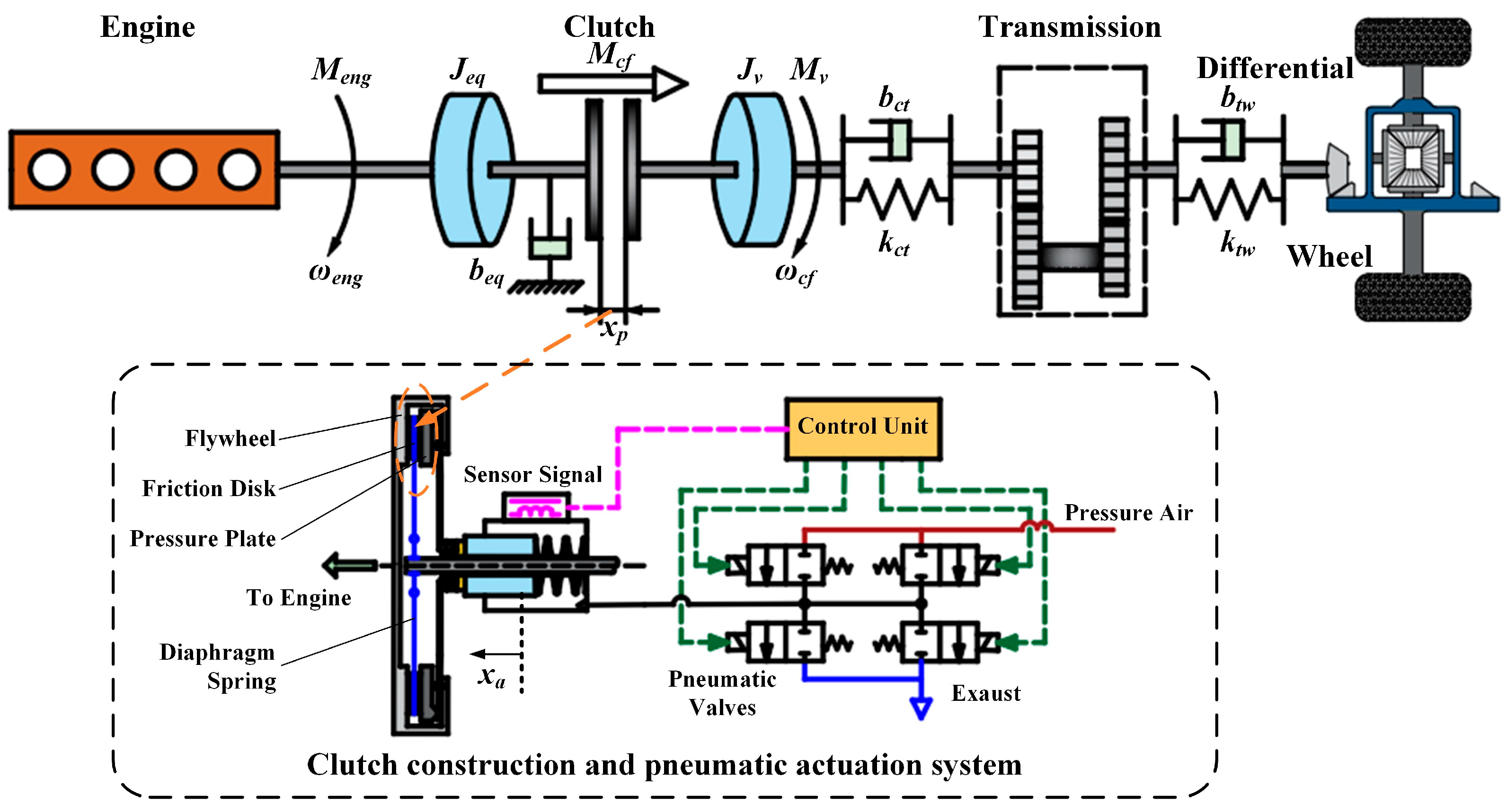
2.1. Vehicle Launching Clutch Dynamics Analysis
- (1)
- Clutch empty stroke stage
- (2)
- Clutch slipping stage
- (3)
- Clutch synchronization stage
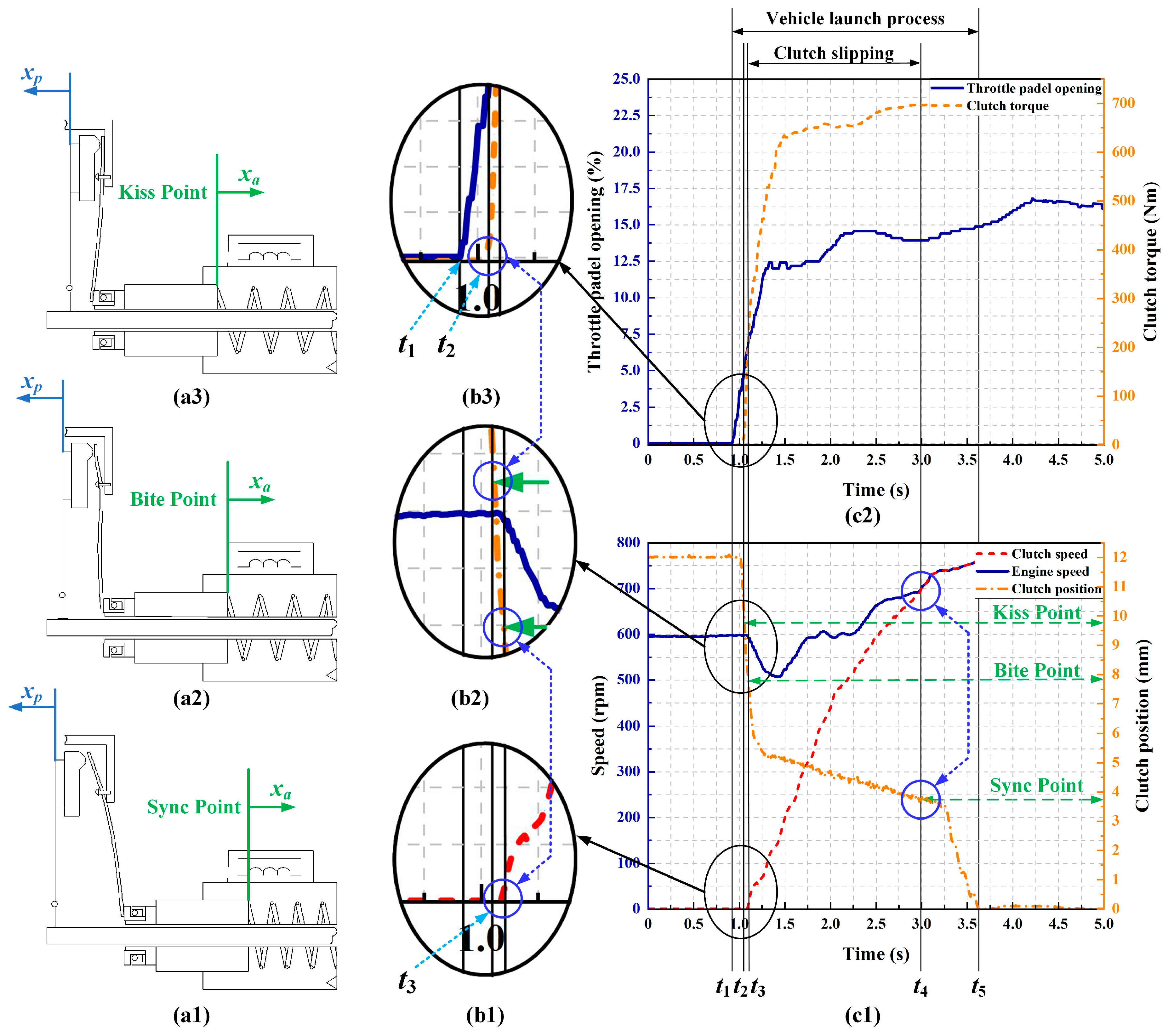
2.2. Vehicle Launching Clutch Engagement Displacement Change
- (1)
- Time point t1
- (2)
- Time point t2
- (3)
- Time point t3
- (4)
- Time point t4
- (5)
- Time point t5
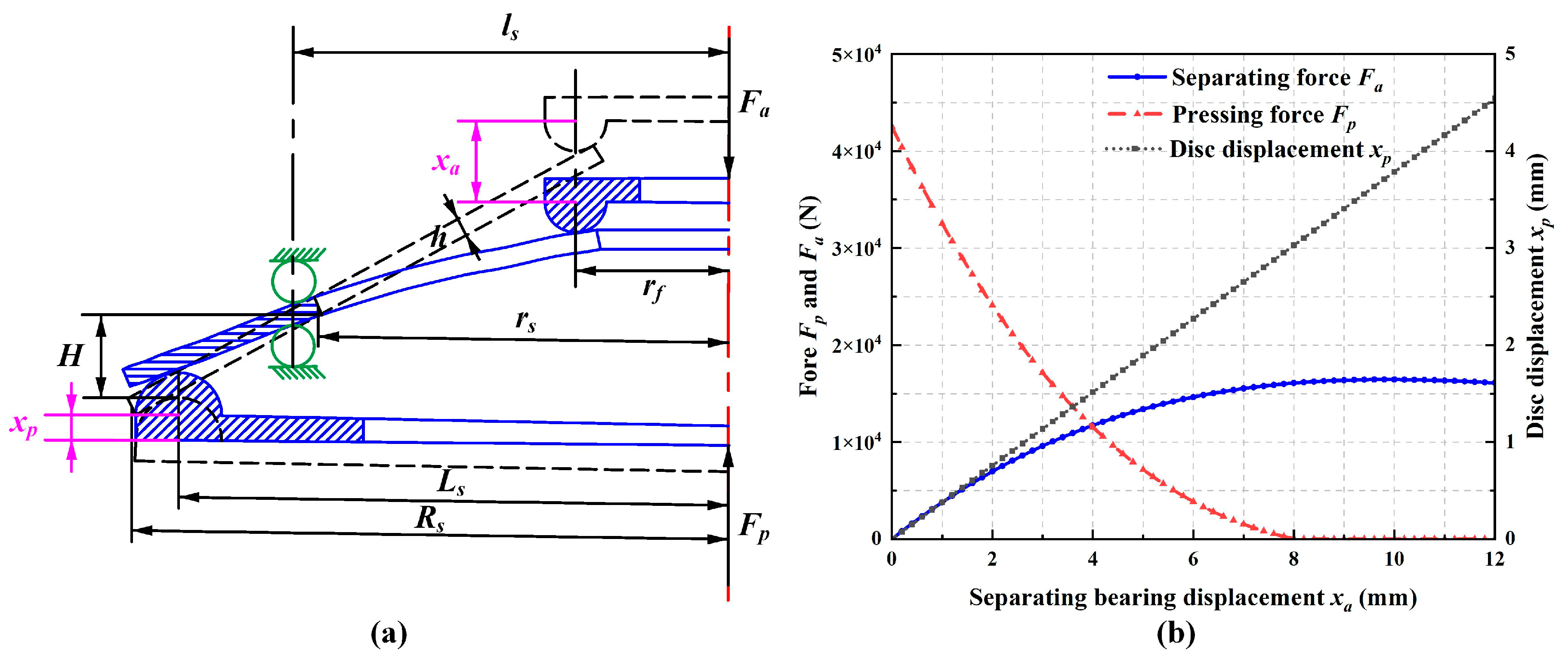
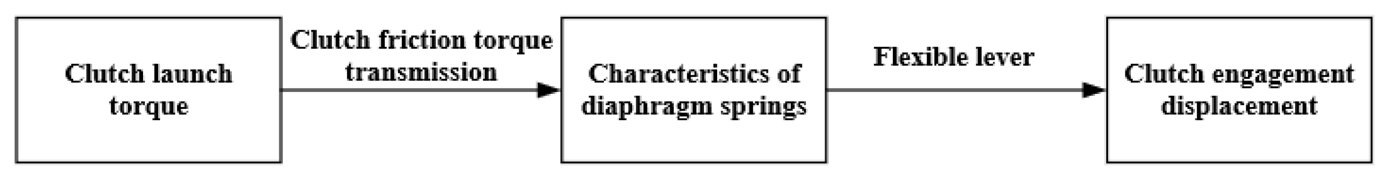
2.3. Relationship between Clutch Torque and Displacement
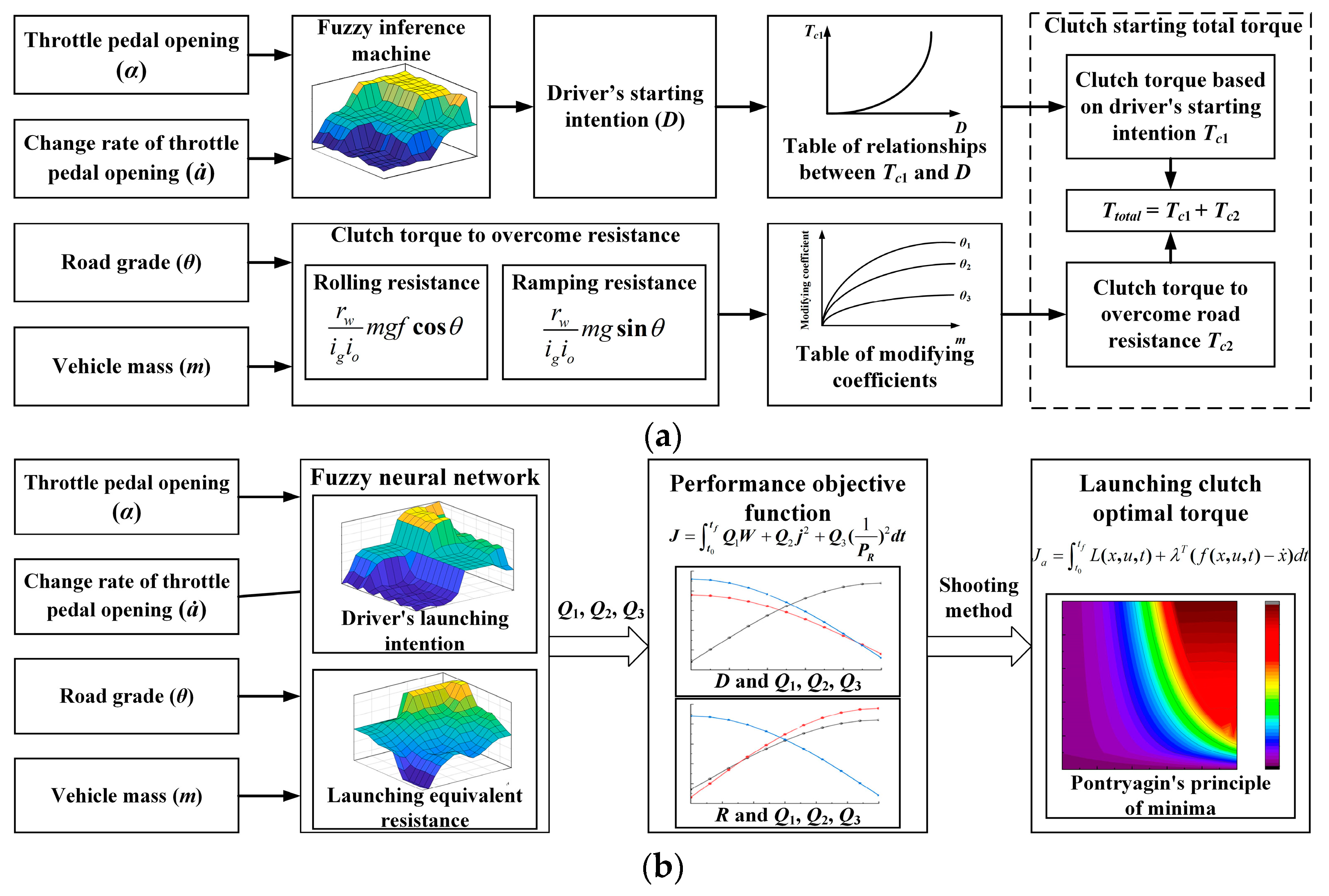
3. Launching States Recognition (LSR) for Clutch Torque
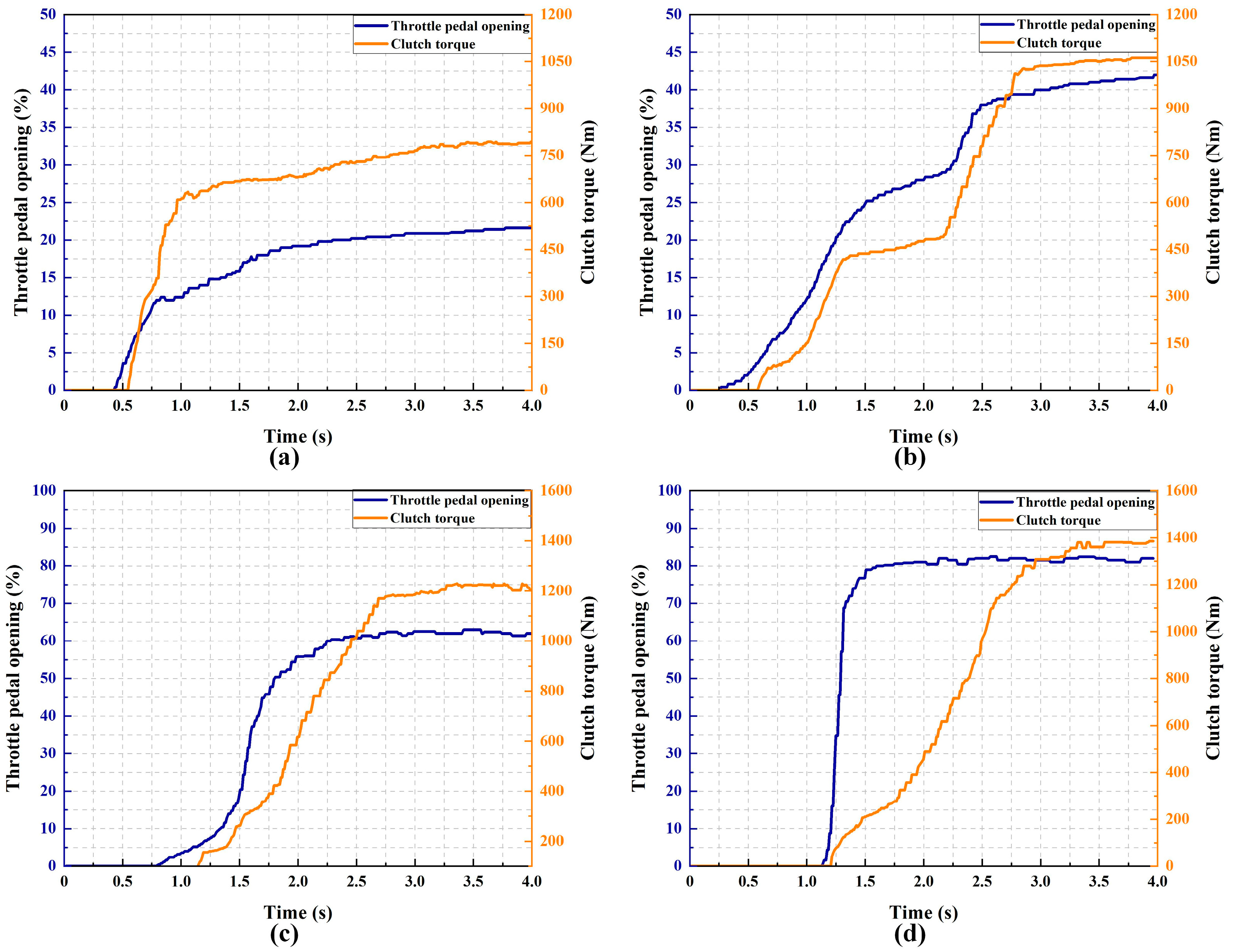
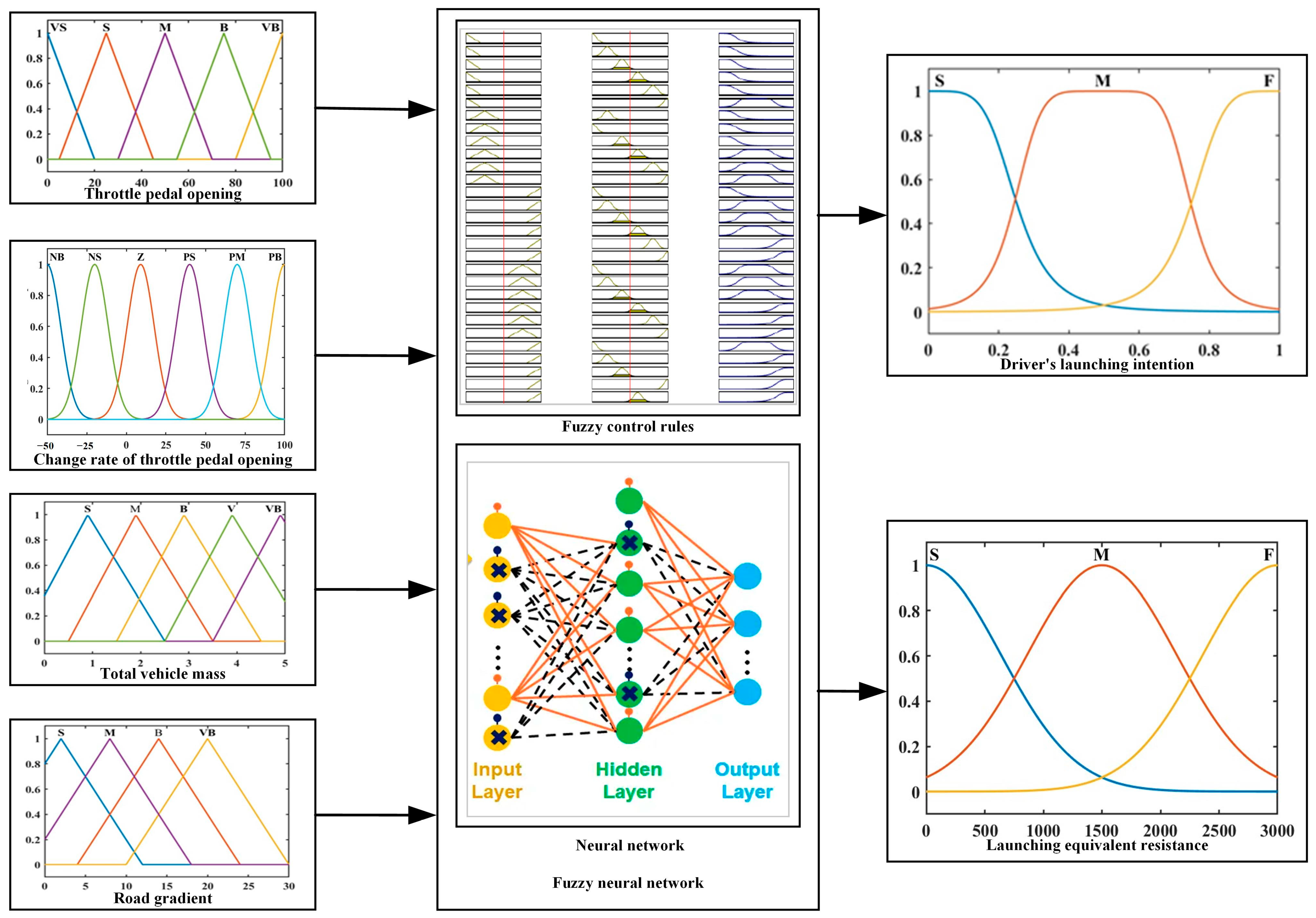
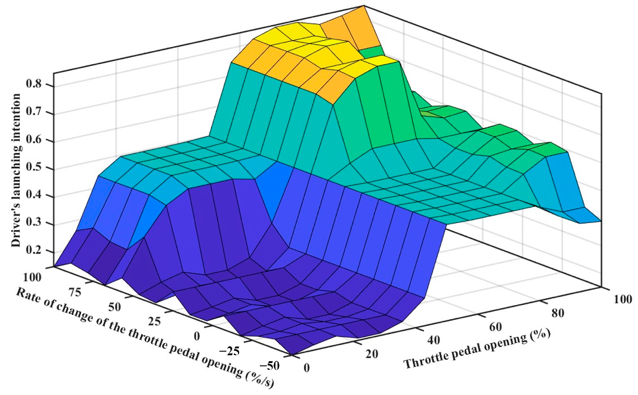
3.1. Driver’s Launching Intention Recognition
- (1)
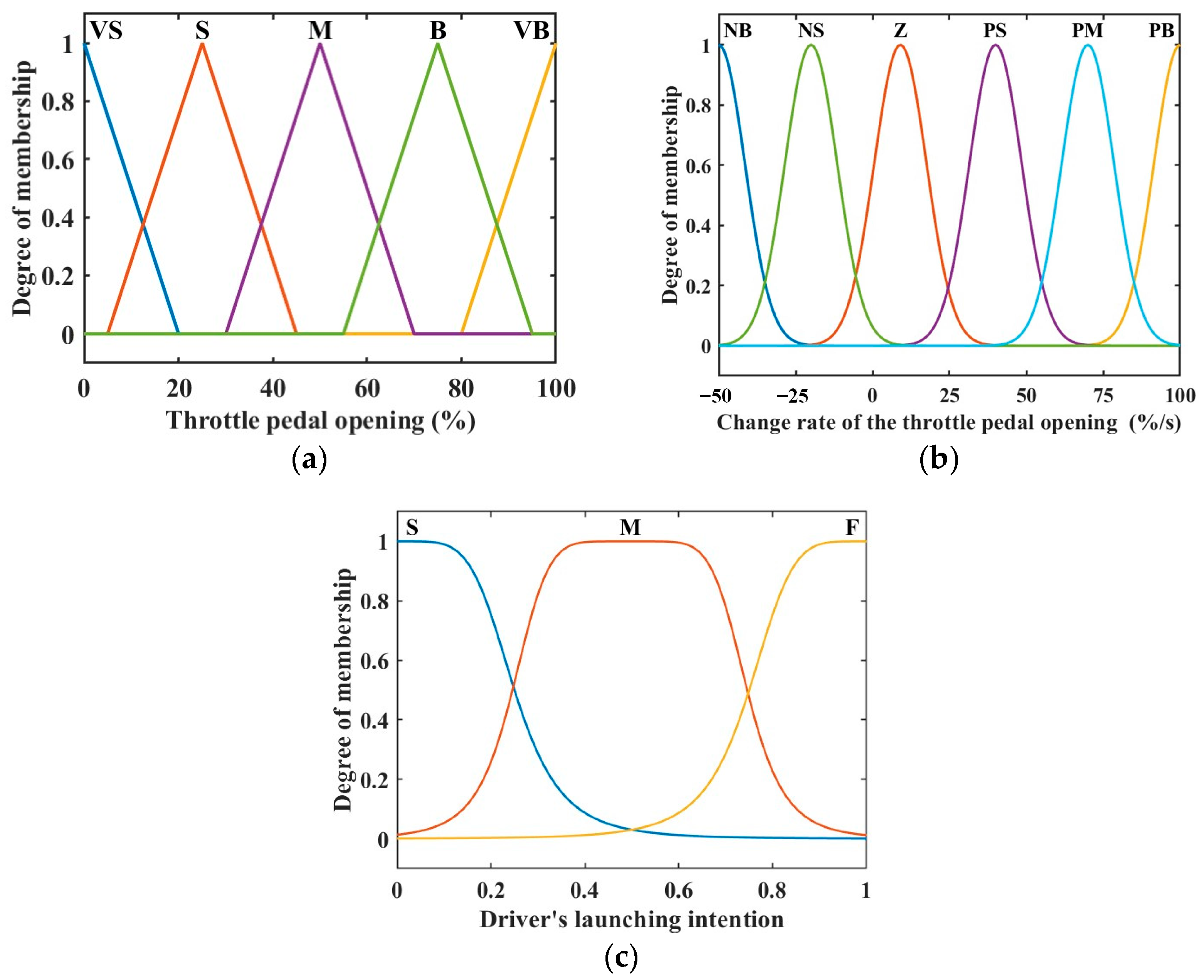
- Fuzzy domain division of throttle pedal opening and definition of fuzzy subset
- (2)
- Fuzzy domain division and fuzzy subset definition for change rate of throttle pedal opening
- (3)
- Driver’s launching intentions fuzzy domain delineation and fuzzy subset definition
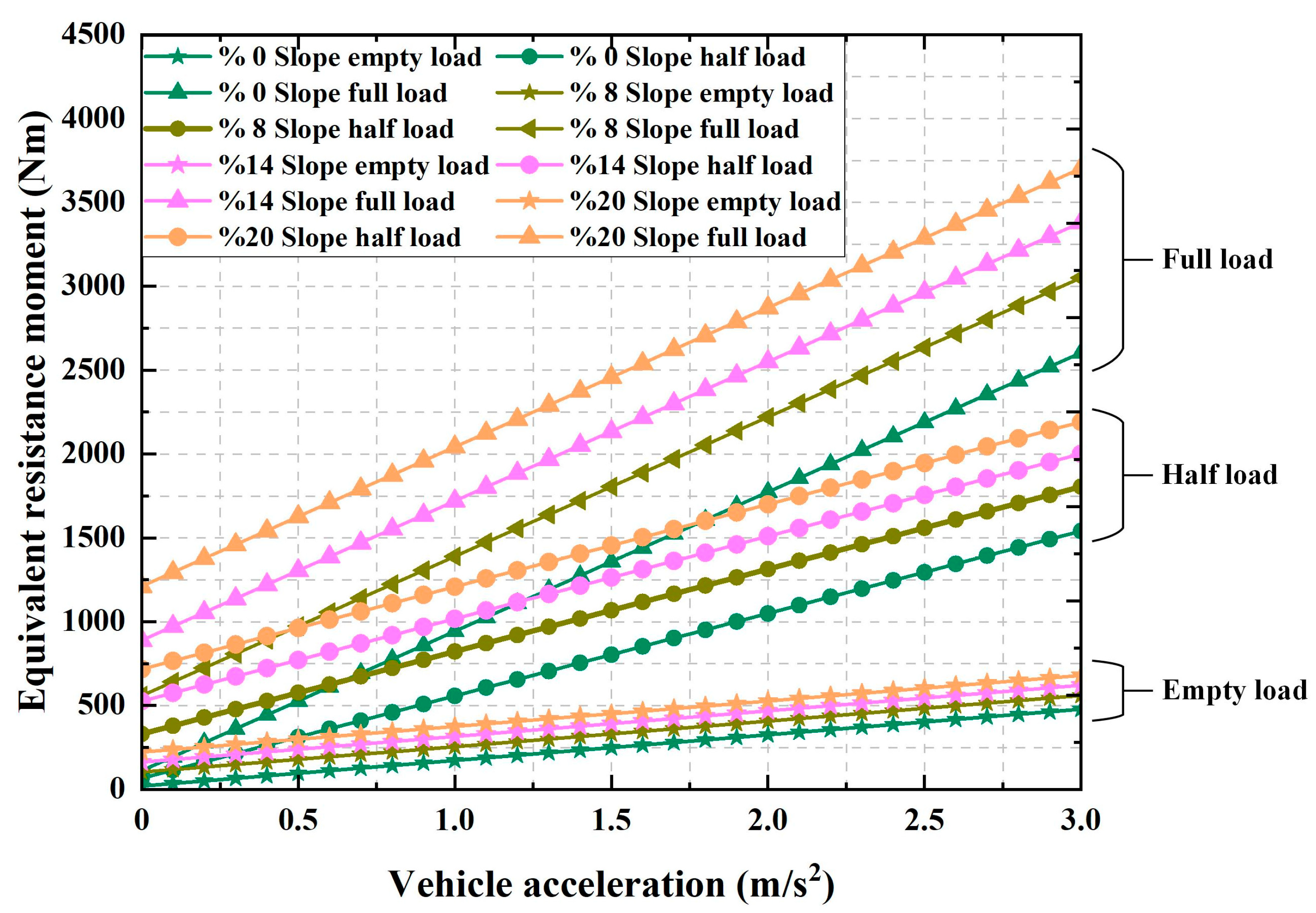
3.2. Launching Equivalent Resistance Recognition
- (1)
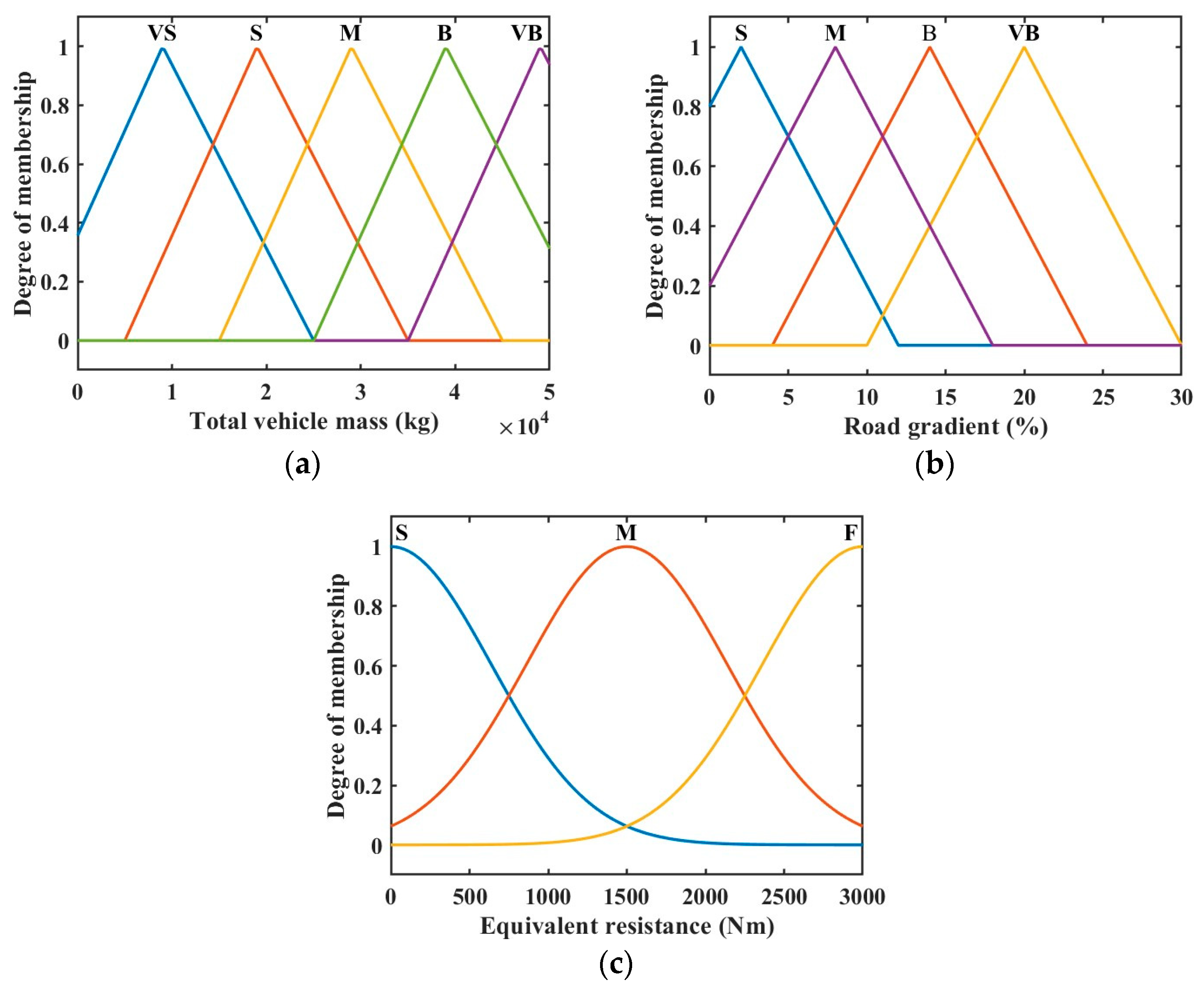
- Total vehicle mass fuzzy domain delineation and fuzzy subset definition
- (2)
- Road gradient fuzzy domain delineation and fuzzy subset definition
- (3)
- Launching equivalent resistance fuzzy domain division and fuzzy subset definition
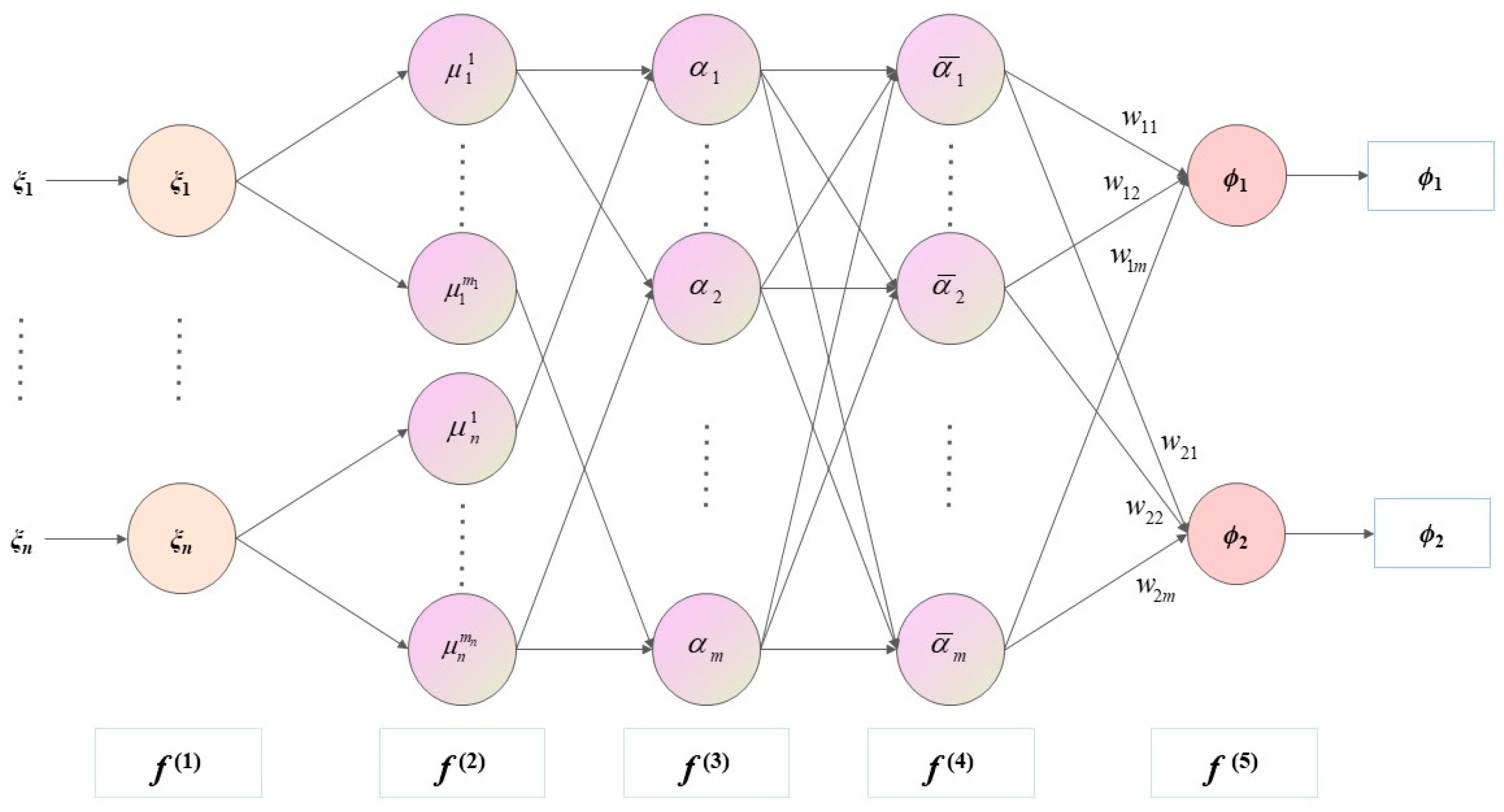
3.3. Fuzzy Neural Network-Based Launching States Recognition
4. Optimum Clutch Torque Control for Launching
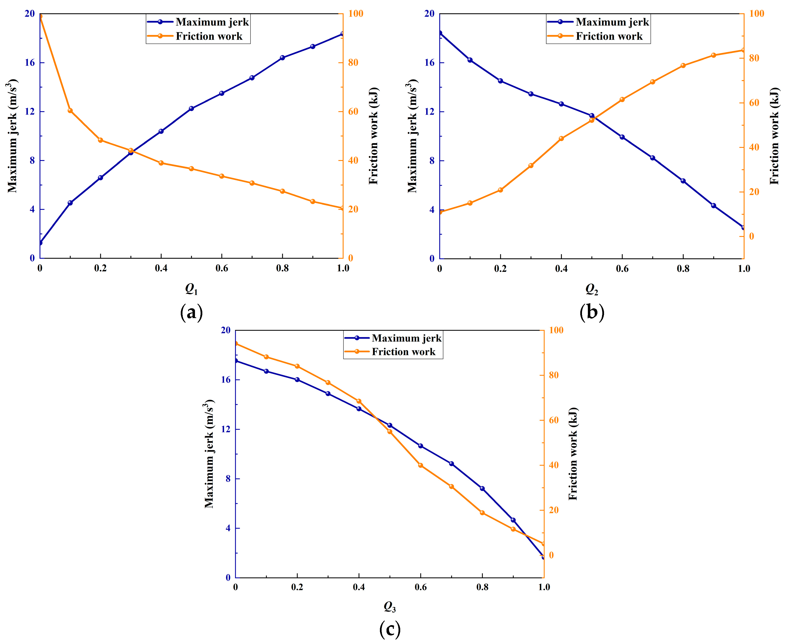
4.1. Performance Evaluation Indexes
4.2. Description of the Launching Optimal Control Problem
4.3. Shooting Method for Solving Launch Optimal Control Problems
- (1)
- State equation:
- (2)
- Co-state equation:
- (3)
- Control equation:
- (4)
- Boundary conditions:
- (5)
- Constraints:
- (6)
- Transversality condition:
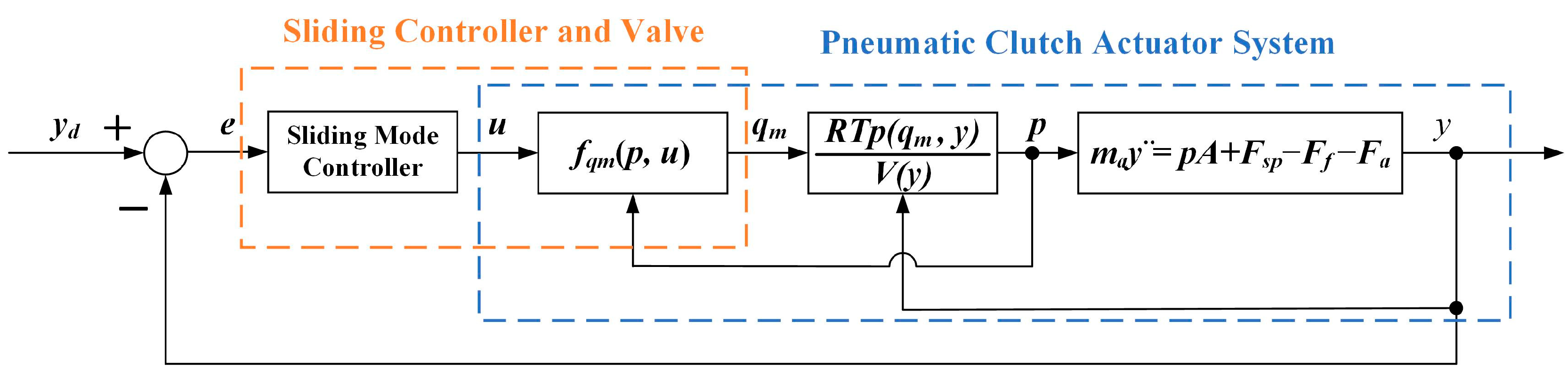
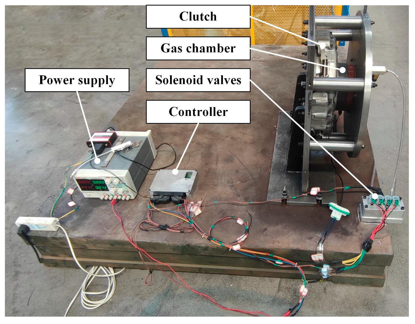
4.4. Clutch Pneumatic Actuator Control
- Mode 1 (u = 1): gas enters the working chamber;
- Mode 2 (u = −1): gas is exhausted from the working chamber;
- Mode 3 (u = 0): the working chamber is closed.
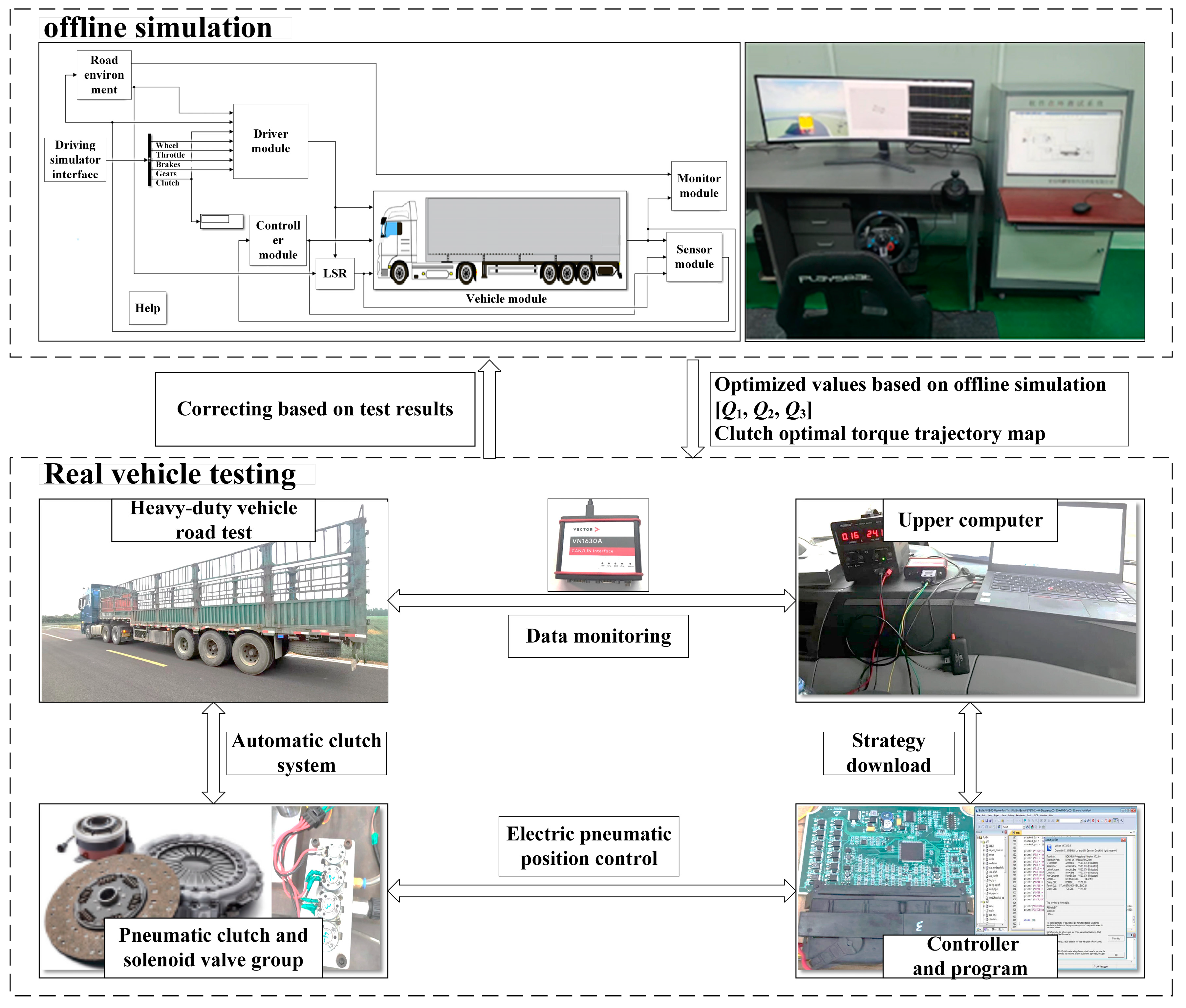
5. Simulation and Experimental Analysis
5.1. Design of Simulations and Experiments
5.2. Analysis and Discussion of Results
6. Conclusions
Author Contributions
Funding
Data Availability Statement
Conflicts of Interest
References
- Della Gatta, A.; Iannelli, L.; Pisaturo, M.; Senatore, A.; Vasca, F. A survey on modeling and engagement control for automotive dry clutch. Mechatronics 2018, 55, 63–75. [Google Scholar] [CrossRef]
- Pan, T.; Zang, H.Q. Position-based impedance torque control for automatic clutch with robust predefined-time stability guarantee. Proc. Inst. Mech. Eng. Part I J. Syst. Control. Eng. 2023, 237, 1542–1557. [Google Scholar] [CrossRef]
- Wu, J.M.; Yan, H.Z.; Liu, S.Q.; Ni, D. Study on nonlinear dynamics characteristics of dual speed dual clutch transmission system based on bond graph. Heliyon 2023, 9, e20862. [Google Scholar] [CrossRef] [PubMed]
- Zhao, Z.G.; Chen, H.J.; Zhen, Z.X.; Yang, Y.Y. Optimal torque coordinating control of the launching with twin clutches simultaneously involved for dry dual-clutch transmission. Veh. Syst. Dyn. 2014, 52, 776–801. [Google Scholar] [CrossRef]
- Yang, Y.Y.; Zhu, Z.B.; Wang, X.Y.; Chen, Z.; Ma, Z.L. Optimal launching-intention-aware control strategy for automated clutch engagement. Int. J. Automot. Technol. 2017, 18, 417–428. [Google Scholar] [CrossRef]
- Li, L.; Zhu, Z.B.; Chen, Y.; He, K.; Li, X.J.; Wang, X.Y. Engagement Control of Automated Clutch for Vehicle Launching Considering the Instantaneous Changes of Driver’s Intention. J. Dyn. Syst. Meas. Control. 2017, 139, 021011. [Google Scholar] [CrossRef]
- Zhao, G.D.; Liu, Y.G.; Zhai, K.N.; Jiang, F.Y.; Huang, Q.; Chen, Z. Research on intelligent launching control of dual clutch transmissions based on adaptive neural fuzzy inference system. J. Mech. Sci. Technol. 2022, 36, 3227–3237. [Google Scholar] [CrossRef]
- Liu, Y.G.; Zhang, J.C.; Huang, Q.; Chen, Z.; Chen, Z.H. Optimal Clutch Torque Prediction for Shifting Process of Dual Clutch Transmission Based on Support Vector Regression. Int. J. Automot. Technol. 2022, 23, 1073–1084. [Google Scholar] [CrossRef]
- Lin, X.Y.; Li, Y.L.; Xia, B. An online driver behavior adaptive shift strategy for two-speed AMT electric vehicle based on dynamic corrected factor. Sustain. Energy Technol. 2021, 48, 101598. [Google Scholar] [CrossRef]
- Liu, Y.G.; Zhao, P.; Qin, D.T.; Li, G.; Chen, Z.; Zhang, Y. Driving Intention Identification Based on Long Short-Term Memory and A Case Study in Shifting Strategy Optimization. IEEE Access 2019, 7, 128593–128605. [Google Scholar] [CrossRef]
- Wang, D.Y.; Hu, M.H.; Li, B.G.; Qin, D.T.; Sun, D.Y. Modular modeling and dynamic response analysis of a driveline system during start-up process. Mech. Mach. Theory 2021, 156, 104136. [Google Scholar] [CrossRef]
- Park, J.; Choi, S. Optimization Method of Reference Slip Speed in Clutch Slip Engagement in Vehicle Powertrain. Int. J. Automot. Technol. 2021, 22, 55–67. [Google Scholar] [CrossRef]
- Xu, Z.Y.; Liu, H.J. Research on the identification of DCT vehicle driver’s starting intention based on LSTM neural network and multi-sensor data fusion. Proc. Inst. Mech. Eng. Part D J. Automob. Eng. 2023, 237, 2928–2941. [Google Scholar] [CrossRef]
- Feng, J.H.; Qin, D.T.; Liu, Y.G.; Wang, X.; Lv, H. Pseudo-spectral optimization and data-driven control of vehicle start process with dual-clutch transmission. Mech. Mach. Theory 2022, 172, 104814. [Google Scholar] [CrossRef]
- Gao, J.; Yin, C.Q.; Jiang, C. Research on clutch position control based on backstepping method for small-sized tractors. Sci. Prog. 2023, 106. [Google Scholar] [CrossRef] [PubMed]
- Dong, G.; Wang, F.; Meng, D.L.; Chu, H.Q.; Hong, J.L.; Gao, B.Z. Modeling and control of ball-ramp electromechanical clutch actuator for in-wheel AMT of electric vehicles. Mech. Mach. Theory 2023, 180, 25–35. [Google Scholar] [CrossRef]
- Wu, P.; Qiang, P.H.; Pan, T.; Zang, H.Q. Double-Loop Control for Torque Tracking of Dry Clutch. Machines 2022, 10, 1142. [Google Scholar] [CrossRef]
- Liang, J.; Wang, F.; Feng, J.; Zhao, M.; Fang, R.; Pi, D.; Yin, G. A Hierarchical Control of Independently Driven Electric Vehicles Considering Handling Stability and Energy Conservation. IEEE Trans. Intell. Veh. 2024, 9, 738–751. [Google Scholar] [CrossRef]
- Guo, J.; Zhang, Y.Q. Adaptive Starting Control Strategy for Hybrid Electric Vehicles Equipped with a Wet Dual-Clutch Transmission. Actuators 2023, 12, 123. [Google Scholar] [CrossRef]
- Feng, J.H.; Qin, D.T.; Liu, Y.G.; Wang, X.; Lv, H. Pseudo-spectral optimization and model predictive control of vehicle shift process with dual clutch transmission. Proc. Inst. Mech. Eng. Part C J. Mech. Eng. Sci. 2023, 237, 3789–3806. [Google Scholar] [CrossRef]
- Bécsi, T. Quasi-Linear Parameter Varying Modeling and Control of an Electromechanical Clutch Actuator. Mathematic 2022, 10, 1473. [Google Scholar] [CrossRef]
- Ding, J.A.; Jiao, X.H. Observer-based adaptive dynamic sliding mode control for automatic clutch position tracking. Proc. Inst. Mech. Eng. Part E J. Process. Mech. Eng. 2023. [Google Scholar] [CrossRef]
- Yuan, R.F.; Wu, G.Q.; Shao, C.H.; Su, S.Q. Mechanism-oriented control for suppressing start-up judder of vehicle with automatic dry clutch: Experiment and simulation analysis. Proc. Inst. Mech. Eng. Part D J. Automob. Eng. 2021, 235, 744–758. [Google Scholar] [CrossRef]
- Wang, B.; Gao, B.Z.; Chen, H. Adaptive Optimal Control of Starting-up of Automated Manual Transmission. In Proceedings of the 2014 11th World Congress on Intelligent Control and Automation (Wcica), Shenyang, China, 29 June–4 July 2014; pp. 1723–1728. [Google Scholar]
- Gao, B.Z.; Hong, J.L.; Qu, T.; Yu, S.Y.; Chen, H. An Output Regulator With Rejection of Time-Varying Disturbance: Experimental Validation on Clutch Slip Control. IEEE Trans. Control. Syst. Technol. 2020, 28, 1158–1167. [Google Scholar] [CrossRef]
- Yang, Y.; Wang, M.M.; Xia, F.G.; Qin, D.T.; Feng, J.H. Modeling and Control Approach for Dual Clutch Transmission Vehicles Starting Process Based on State-Dependent Autoregressive With Exogenous Model. IEEE Access 2020, 8, 158712–158726. [Google Scholar] [CrossRef]
- Hong, J.L.; Gao, B.Z.; Yue, H.Q.; Chen, H. Dry Clutch Control of Two-Speed Electric Vehicles by Using an Optimal Control Scheme With Persistent Time-Varying Disturbance Rejection. IEEE Trans. Transp. Electrif. 2021, 7, 2034–2046. [Google Scholar] [CrossRef]
- Meng, F.; Chen, H.Y.; Zhang, T.; Zhu, X.Y. Clutch fill control of an automatic transmission for heavy-duty vehicle applications. Mech. Syst. Signal Process. 2015, 64–65, 16–28. [Google Scholar] [CrossRef]
- Kim, S.; Shin, K.; Yoo, C.; Huh, K. Development of Algorithms for Commercial Vehicle Mass and Road Grade Estimation. Int. J. Automot. Technol. 2017, 18, 1077–1083. [Google Scholar] [CrossRef]
- Cai, L.L.; Wang, H.L.; Jia, T.L.; Peng, P.; Pi, D.W.; Wang, E.L. Two-layer structure algorithm for estimation of commercial vehicle mass. Proc. Inst. Mech. Eng. Part D J. Automob. Eng. 2020, 234, 378–389. [Google Scholar] [CrossRef]
- Liu, Y.C.; Wei, L.T.; Fan, Z.X.; Wang, X.Y.; Li, L. Road slope estimation based on acceleration adaptive interactive multiple model algorithm for commercial vehicles. Mech. Syst. Signal Proc. 2023, 184, 109733. [Google Scholar] [CrossRef]
- Zheng, W.G.; Zhang, J.Z.; Wang, S.C.; Feng, G.S.; Xu, X.H.; Ma, Q.X. A Shifting Strategy for Electric Commercial Vehicles Considering Mass and Gradient Estimation. Comput. Model. Eng. Sci. 2023, 137, 489–508. [Google Scholar] [CrossRef]
- Kim, J. Real-Time Torque Estimation of Automotive Powertrain With Dual-Clutch Transmissions. IEEE Trans. Control. Syst. Technol. 2022, 30, 2269–2284. [Google Scholar] [CrossRef]
- Shi, J.L.; Li, L.; Wang, X.Y.; Liu, C.Z. Robust output feedback controller with high-gain observer for automatic clutch. Mech. Syst. Signal Proc. 2019, 132, 806–822. [Google Scholar] [CrossRef]
- Li, Y.X.; Wang, Z.C. Motion Characteristics of a Clutch Actuator for Heavy-Duty Vehicles with Automated Mechanical Transmission. Actuators 2021, 10, 179. [Google Scholar] [CrossRef]
- Guo, X.L.; Lu, H.M. Optimal Design on Diaphragm Spring of Automobile Clutch. In Proceedings of the Icicta: 2009 Second International Conference on Intelligent Computation Technology and Automation, Changsha, China, 10–11 October 2009; Volume III, pp. 206–208. [Google Scholar] [CrossRef]
- ISO 6358-3:2013; Pneumatic Fluid Power—Determination of Flow-Rate Characteristics of Components Using Compressible Fluids—Part 3: Method for Calculating Steady-State Flow-Rate Characteristics of Systems. ISO Internationale Organisation: Switzerland, Geneva, 2013.
- Qian, P.F.; Liu, L.; Pu, C.W.; Meng, D.Y.; Páez, L.M.R. Methods to improve motion servo control accuracy of pneumatic cylinders-review and prospect. Int. J. Hydromechatronics 2023, 6, 274–310. [Google Scholar] [CrossRef]
- Li, L.; Zhu, Z.B.; Wang, X.Y.; Yang, Y.Y.; Yang, C.; Song, J. Identification of a driver’s starting intention based on an artificial neural network for vehicles equipped with an automated manual transmission. Proc. Inst. Mech. Eng. Part D. J. Automob. Eng. 2016, 230, 1417–1429. [Google Scholar] [CrossRef]
- Torabi, S.; Wahde, M.; Hartono, P. Road Grade and Vehicle Mass Estimation for Heavy-duty Vehicles Using Feedforward Neural Networks. In Proceedings of the 2019 4th International Conference on Intelligent Transportation Engineering (Icite 2019), Singapore, 5–7 September 2019; pp. 316–321. [Google Scholar] [CrossRef]
- Chen, R.; Sun, D.Y. Fuzzy Neural Network Control of AMT Clutch in Starting Phase. In Proceedings of the 2008 International Symposium on Intelligent Information Technology Application, Shanghai, China, 20–22 December 2008; Volume II, pp. 712–715. [Google Scholar] [CrossRef]
- Li, A.T.; Qin, D.T. Adaptive model predictive control of dual clutch transmission shift based on dynamic friction coefficient estimation. Mech. Mach. Theory 2022, 173, 104804. [Google Scholar] [CrossRef]
- Xie, S.B.; Hu, X.S.; Lang, K.; Qi, S.W.; Liu, T. Powering Mode-Integrated Energy Management Strategy for a Plug-In Hybrid Electric Truck with an Automatic Mechanical Transmission Based on Pontryagin’s Minimum Principle. Sustainability 2018, 10, 3758. [Google Scholar] [CrossRef]
- Qian, P.F.; Ren, X.D.; Tao, G.L.; Zhang, L.R. Compound Sliding Mode Motion Trajectory Tracking Control of an Electro-Pneumatic Clutch Actuator While Maximizing Its Stiffness. J. Chin. Soc. Mech. Eng. 2016, 37, 515–524. [Google Scholar]
- Myklebust, A.; Eriksson, L. Modeling, Observability, and Estimation of Thermal Effects and Aging on Transmitted Torque in a Heavy Duty Truck With a Dry Clutch. IEEE/ASME Trans. Mechatron. 2015, 20, 61–72. [Google Scholar] [CrossRef]


| Parameter Name | Value | Parameter Name | Value |
|---|---|---|---|
| Modulus of elasticity E | 2.06 × 10⁵ Mpa | Radius of the small end rs | 141 mm |
| Poisson’s ratio μs | 0.29 | Radius of the large end Rs | 205.5 mm |
| Thickness of steel plate h | 5.3 mm | Radius of platen loading point Ls | 195 mm |
| Height of inner cut-off cone of disc spring H | 8.6 mm | Radius of support ring loading point ls | 156 mm |
| Separate bearing load point radius rf | 53 mm |
| Throttle Pedal Opening (%) | Change Rate of the Throttle Pedal Opening (%·s−1) | |||||
|---|---|---|---|---|---|---|
| NB | NS | Z | PS | PM | PB | |
| VS | S | S | S | S | S | S |
| S | S | S | S | S | M | M |
| M | S | M | M | M | M | F |
| B | M | M | M | F | F | F |
| VB | M | F | F | F | F | F |
| Total Vehicle Mass (kg) | Road Gradient (%) | |||
|---|---|---|---|---|
| S | M | B | VB | |
| S | S | S | S | M |
| M | S | S | M | F |
| B | S | M | M | F |
| V | M | M | F | F |
| VB | M | F | F | F |
| Parameter Name | Value | |
|---|---|---|
| Vehicle parameters | A heavy-duty vehicle empty/half/full load mass | 9000/29,000/49,000 kg |
| Rolling resistance coefficient | 0.015 | |
| Windward area | 9.56 m2 | |
| Wind resistance factor | 0.76 | |
| Engine parameters | Maximum output power | 413 Kw |
| Maximum output torque | 2600 Nm | |
| Rated speed | 1800 rpm | |
| Clutch and AMT parameters | Clutch torque capacity | 3000 Nm |
| Clutch friction coefficient | 0.3 | |
| AMT maximum input torque | 2600 Nm | |
| Transmission 1st/2nd/3rd gear ratio | 16.688/12.924/9.926 | |
| Driveline efficiency | 96% | |
| Main reducer ratio | 2.867 | |
| Wheel radius | 0.537 m | |
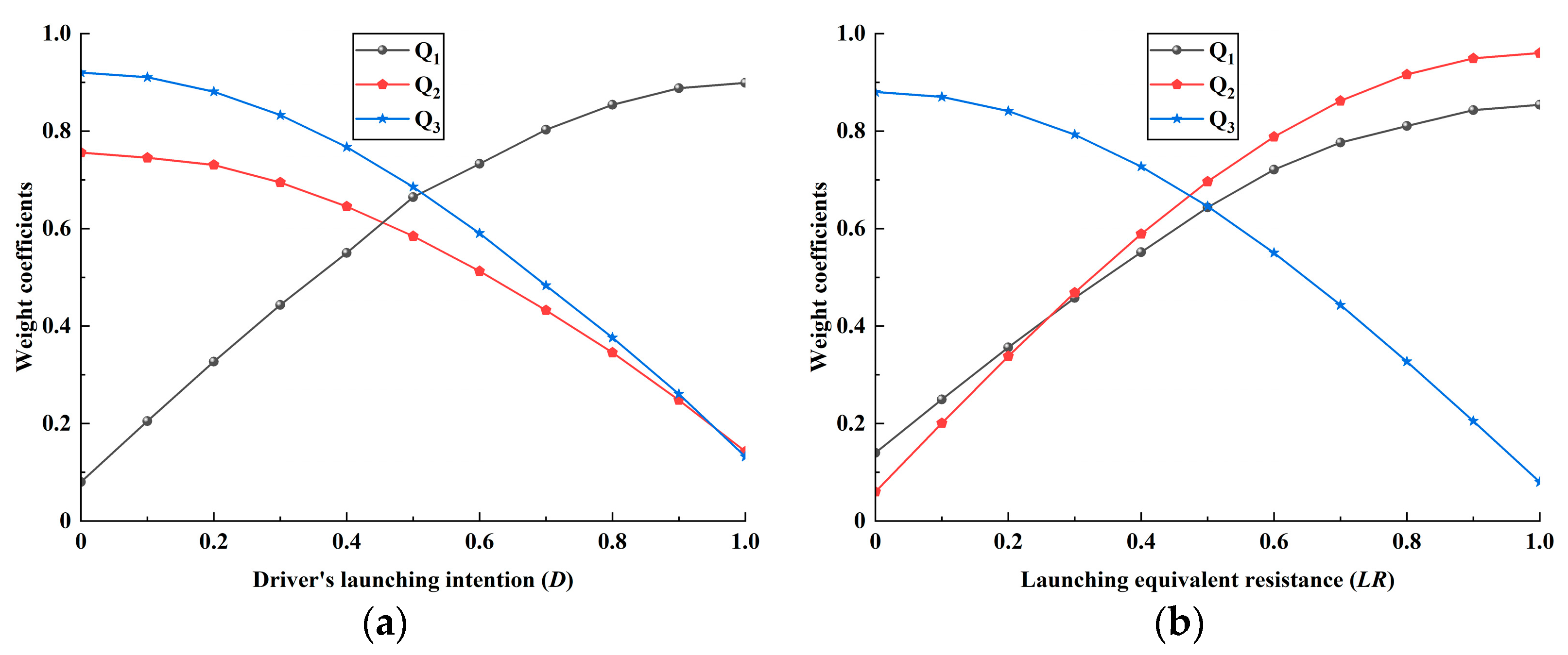
| D | Jerk (j) | Friction Work (W) | The Weighting Coefficients (Q) | LR | Jerk (j) | Friction Work (W) | The Weighting Coefficients (Q) |
|---|---|---|---|---|---|---|---|
| {S} | Small | Large | [Q1 is small, Q2 is large, Q3 is large] | {S} | Small | Small | [Q1 is small, Q2 is small, Q3 is large] |
| {M} | Middle | Middle | [Q1 is middle, Q2 is middle, Q3 is middle] | {M} | Middle | Middle | [Q1 is middle, Q2 is middle, Q3 is middle] |
| {F} | Large | Small | [Q1 is large, Q2 is small, Q3 is small] | {F} | Large | Large | [Q1 is large, Q2 is large, Q3 is small] |
| Case Type | Driver’s Launching Intentions | Launching Equivalent Resistance Torque | Torque Control Strategy | |
|---|---|---|---|---|
| Case 1-1 | α = [0%~30%], m = 9000 kg, θ = 0% | Slow speed | Small resistance | Without optimal strategy |
| Case 1-2 | Slow speed | Small resistance | Optimal control strategy | |
| Case 2-1 | α = [0%~55%], m = 29,000 kg, θ = 8% | Middle speed | Middle resistance | Without optimal strategy |
| Case 2-2 | Middle speed | Middle resistance | Optimal control strategy | |
| Case 3-1 | α = [0%~100%], m = 49,000 kg, θ = 20% | Fast speed | Large resistance | Without optimal strategy |
| Case 3-2 | Fast speed | Large resistance | Optimal control strategy | |
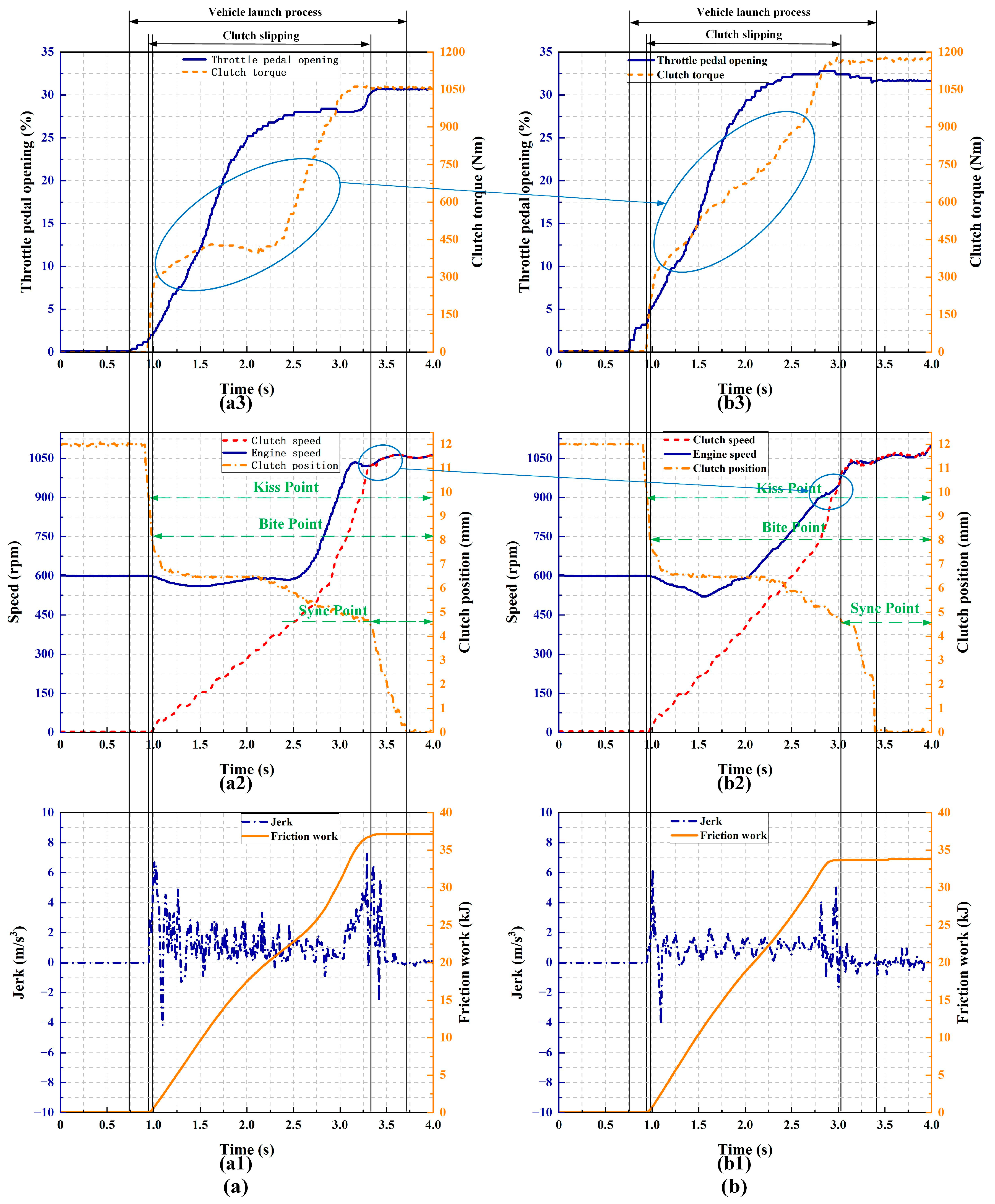
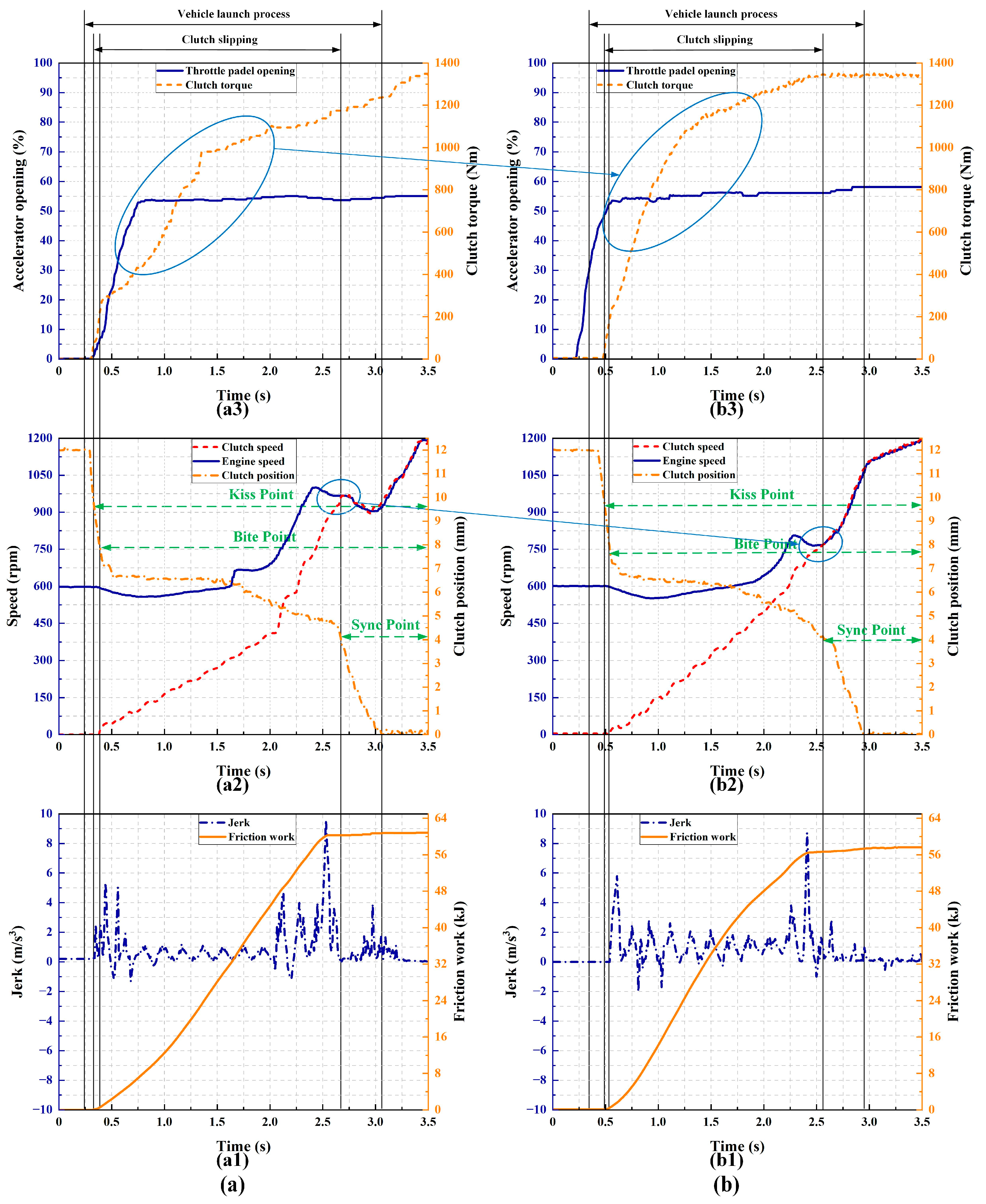
| Case Type | Maximum Jerk j (m/s3) | Friction Work W (kJ) | Speed Sync Time t (s) |
|---|---|---|---|
| Case1-1 | 7.251 | 37.146 | 2.312 |
| Case1-2 | 6.212 | 33.821 | 2.061 |
| Improvement | 14.33% | 8.95% | 10.86% |
| Case2-1 | 9.588 | 60.853 | 2.276 |
| Case2-2 | 8.726 | 57.644 | 2.101 |
| Improvement | 8.99% | 5.27% | 7.69% |
| Case3-1 | 14.713 | 75.348 | 2.234 |
| Case3-2 | 11.254 | 74.412 | 2.121 |
| Improvement | 23.51% | 1.24% | 5.06% |
| Case Type | Kiss Point (mm) | Bite Point (mm) | Sync Point (mm) |
|---|---|---|---|
| Case1-1 | 9.779 | 8.211 | 4.677 |
| Case1-2 | 9.843 | 8.106 | 4.572 |
| Case2-1 | 9.833 | 7.807 | 4.086 |
| Case2-2 | 9.779 | 7.539 | 3.891 |
| Case3-1 | 9.786 | 7.245 | 3.544 |
| Case3-2 | 9.837 | 7.058 | 3.155 |
Disclaimer/Publisher’s Note: The statements, opinions and data contained in all publications are solely those of the individual author(s) and contributor(s) and not of MDPI and/or the editor(s). MDPI and/or the editor(s) disclaim responsibility for any injury to people or property resulting from any ideas, methods, instructions or products referred to in the content. |
© 2024 by the authors. Licensee MDPI, Basel, Switzerland. This article is an open access article distributed under the terms and conditions of the Creative Commons Attribution (CC BY) license (https://creativecommons.org/licenses/by/4.0/).
Share and Cite
Geng, X.; Liu, W.; Liu, X.; Wen, G.; Xue, M.; Wang, J. Optimal Torque Control of the Launching Process with AMT Clutch for Heavy-Duty Vehicles. Machines 2024, 12, 363. https://doi.org/10.3390/machines12060363
Geng X, Liu W, Liu X, Wen G, Xue M, Wang J. Optimal Torque Control of the Launching Process with AMT Clutch for Heavy-Duty Vehicles. Machines. 2024; 12(6):363. https://doi.org/10.3390/machines12060363
Chicago/Turabian StyleGeng, Xiaohu, Weidong Liu, Xiangyu Liu, Guanzheng Wen, Maohan Xue, and Jie Wang. 2024. "Optimal Torque Control of the Launching Process with AMT Clutch for Heavy-Duty Vehicles" Machines 12, no. 6: 363. https://doi.org/10.3390/machines12060363
APA StyleGeng, X., Liu, W., Liu, X., Wen, G., Xue, M., & Wang, J. (2024). Optimal Torque Control of the Launching Process with AMT Clutch for Heavy-Duty Vehicles. Machines, 12(6), 363. https://doi.org/10.3390/machines12060363