An Integrated C⁴-Spline Interpolation and Time-Free Global Optimization Methodology Applied to High-Speed Cam Motion Design

Abstract

The optimal tuning of high-order motion parameters has emerged as a promising strategy for actively controlling the kinematics/dynamics of high-speed cam mechanisms. However, accomplishing this task remains challenging with current low-order interpolation or tuning methods. This study proposes an integrated high-order interpolation and tuning methodology for the optimal construction of high-speed motion curves. Initially, an explicit C⁴-spline interpolant (C4SI) is developed. This interpolant utilizes four-order continuous (C⁴) splines to synthesize a high-fidelity motion curve that satisfies the predefined motion constraints up to the fourth order, including dimensionless displacement, velocity, acceleration, jerk, and quirk. Concerning the reduction of motion peaks, a unique C4SI-based global kinematics optimization strategy is designed, using the definite integral of the motion curve (free of the time variable) as the objective function. This facile time-free optimization strategy could yield a simultaneous reduction in multiple motion peaks (up to five), which is currently inaccessible with conventional motion tuning strategies. Concerning the improvement of dynamic characteristics, the C4SI-based time-free global dynamics optimization of variable motion parameters is further performed. The results indicate that the optimized fourth-order motion curve offers minimal high-speed transmission error and residual vibration over the whole rise-dwell-return-dwell cycle, which outperforms the standard motion curves and other low-order counterparts.

1. Introduction

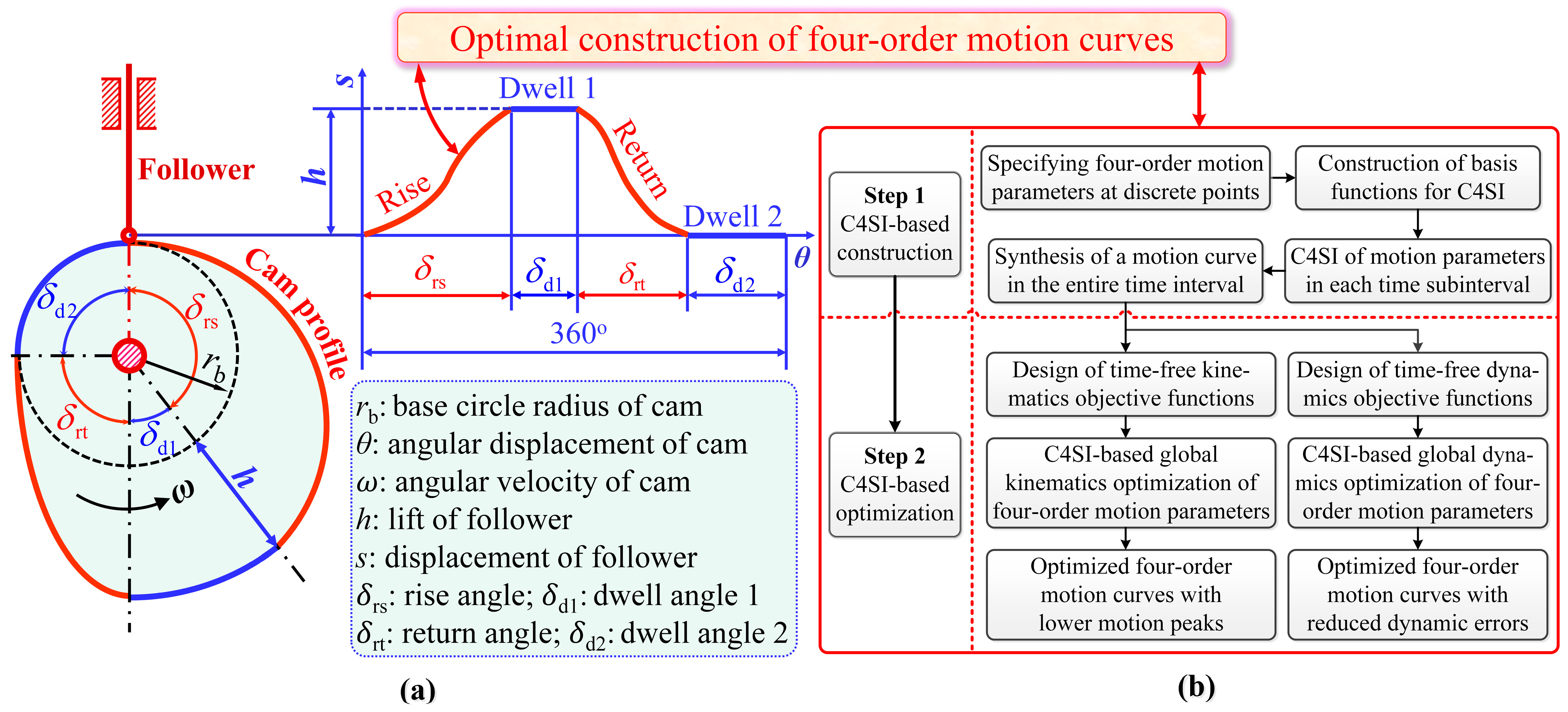
The cam mechanism, as a contact-driven motion unit, plays an integral role in many modern automation machines, such as CNC machining centers [1] and internal combustion engines [2]. The distinct feature of the cam mechanism lies in its ability to tailor the cam profile using predefined transfer functions (termed as motion curves) [3], thus allowing the active control of the follower’s motion to meet case-specific transmission requirements [4], as illustrated in Figure 1a. Hence, the mathematical construction and computational optimization of the motion curve have been long-standing focal points in the development of high-performance cam mechanisms.

In early cam mechanisms, elementary functions (e.g., sine and cosine functions) are commonly adopted as the follower’s motion curves. However, such motion curves often fail to guarantee the desired transmission accuracy or stability for high-speed applications [5]. As such, a series of standard motion curves, including power polynomials, modified sine (MS), the modified constant velocity (MCV) curve, and the modified trapezoidal (MT) curve have been developed and gained widespread acceptance in cam mechanisms [6]. However, recent studies have revealed that standard motion curves still suffer from mathematical defects, such as high-order discontinuities and excessive motion peaks. Such defects can result in unwanted transmission errors, crossover impacts, and residual vibrations, particularly in high-speed scenarios [5,7].

Motivated by the above defects, great efforts have been devoted to the optimal design of alternative motion curves [8,9]. These efforts involve optimal approximation, interpolation, and the tuning (precise manipulation) of discrete motion parameters for specific kinematics/dynamics objectives. For instance, Qiu et al. [10] utilized an enhanced simplex algorithm to optimally tune the control points of uniform B-splines, whereby cam curves with reduced motion peaks and residual vibrations were constructed. Using parameterized cubic/quintic splines, Nguyen and Kim [11] realized the optimal synthesis of flexible cam profiles, which allowed the simultaneous control of velocity and acceleration curves. In addition, piecewise linear, Hermite, and Bezier interpolants have also been adopted in the data-driven reconstruction of cam profiles [12,13]. However, it should be noted that existing cam design studies mostly focus on the basic control of low-order motion parameters, such as displacement (the zeroth derivative), velocity (the first derivative), and acceleration (the second derivative). There have been limited efforts made for the optimal control of the higher-order motion parameters (e.g., the third derivative, jerk, and the fourth derivative, quirk) that are of particular concern in high-speed scenarios. In this regard, Luo et al. [14] recently developed a novel cam design framework that encompassed piecewise high-order interpolant (PHOI), pointwise scaling, and piecewise modulation. This framework allows the free regulation of three-order motion parameters at multiple points but comes with two limitations: (i) the inability to handle higher-order motion constraints (e.g., the fourth derivative, quirk) that limit the tunability and optimization potential of the interpolated motion curve and (ii) the use of non-analytical, time-varying objective functions that result in increased computational difficulties in global kinematics optimization. These limitations can potentially hinder the engineering application of this framework. Therefore, it is of great importance to explore more powerful and efficient strategies for high-speed cam motion design.

The purpose of this study is to precisely control the high-order motion parameters (up to the fourth order), thereby constructing an optimized four-order motion curve for high-speed applications. To this end, we propose an integrated high-order interpolation and tuning methodology. The implementation of this methodology involves two key steps, as illustrated in Figure 1b. In the first step, to break the interpolation limit, an explicit C⁴-spline interpolant (C4SI) is developed using the linear combination of two sets of basis functions to create a C⁴-continuous spline in each time subinterval. Importantly, this C⁴-continuous spline and its derived curves pass through the four-order motion data at the initial and final endpoints. Thus, by sequentially stitching these C⁴-continuous splines, a piecewise motion curve satisfying the predefined four-order motion constraints in the entire time interval can be synthesized. Since this interpolated motion curve can preserve the shape integrity and essential characteristics of the original motion data, it can be described as a shape-preserved curve. In the second step, to further tune the interpolated motion curve, the nodal motion data are parameterized, in part or in whole, and two integral objective functions are designed for global kinematics and dynamics optimizations, respectively. Differing from previous studies using non-analytical, time-varying motion peaks as objective functions [7,14], the designed integral objective functions are analytical and free of dimensionless time or local scaling/modulation variables, which contribute to enhanced computational feasibility and efficiency in global optimization.

The primary contribution of this study lies in the proposed C4SI model that applies to the creation of shape-preserved and divergence-free motion curves connecting massive discrete points, which is currently inaccessible with conventional low-order interpolants (considering the nodal constraints within the first two orders). Another contribution is the design of integral objective functions (free of the time variable) for global kinematics and dynamics optimizations. These unique time-free optimization strategies allow for the facile tuning of multiorder motion parameters at arbitrary time points. These contributions hold general significance for the optimal design of high-speed cam mechanisms and many other automation machines.

2. Modelling of Four-Order Motion Curves

2.1. Development of the C4SI Model

Currently, the optimal tuning of high-order motion parameters has emerged as a promising strategy for the active kinematic/dynamic control of many high-speed transmission systems [15,16]. In terms of cam motion design, the key to the success of this tuning process lies in the accurate interpolation of multiorder motion data to construct a high-fidelity motion curve f(T) that satisfies the following:

$$f(T_i)=S_i,\hspace{0.17em}{f}^{(1)}(T_i)=V_i,\hspace{0.17em}{f}^{(2)}(T_i)=A_i,\hspace{0.17em}{f}^{(3)}(T_i)=J_i,\hspace{0.17em}{f}^{(4)}(T_i)=Q_i,\hspace{0.17em}\cdots ,$$

(1)

where i is the sequence number, T is the dimensionless time in the closed real interval [0, 1], and S_i, V_i, A_i, J_i A_i, and Q_i are, respectively, the dimensionless displacement, velocity, acceleration, jerk, and quirk at the ith time point T_i.

As indicated in Equation (1), the construction of f(T) is a complex high-order interpolation problem involving massive discrete points, which cannot be addressed by continuous interpolants [15] or conventional low-order piecewise interpolants (e.g., piecewise linear/cubic interpolants) [14]. To address the multinode high-order equality constraints (up to the fourth order) in Equation (1), this study proposes a powerful C⁴-spline interpolant (C4SI) model as follows:

$$\begin{array}{l}f(T)\hspace{0.17em}={\displaystyle \sum _{i=1}^{n-1}[S_{i,1},\hspace{0.17em}{V}_{i,1},\hspace{0.17em}{A}_{i,1},\hspace{0.17em}{J}_{i,1},\hspace{0.17em}{Q}_{i,1}]·{[{\alpha }_{i,1}(T),\hspace{0.17em}{\beta }_{i,1}(T),\hspace{0.17em}{\gamma }_{i,1}(T),\hspace{0.17em}{\delta }_{i,1}(T),\hspace{0.17em}{\vartheta }_{i,1}(T)]}^T}{\psi }_i(T)+\\ \hspace{0.17em}\hspace{0.17em}\hspace{0.17em}\hspace{0.17em}\hspace{0.17em}\hspace{0.17em}\hspace{0.17em}\hspace{0.17em}\hspace{0.17em}\hspace{0.17em}\hspace{0.17em}\hspace{0.17em}\hspace{0.17em}\hspace{0.17em}[S_{i,2},\hspace{0.17em}{V}_{i,2},\hspace{0.17em}{A}_{i,2},\hspace{0.17em}{J}_{i,2},\hspace{0.17em}{Q}_{i,2}]·{[{\alpha }_{i,2}(T),\hspace{0.17em}{\beta }_{i,2}(T),\hspace{0.17em}{\gamma }_{i,2}(T),\hspace{0.17em}{\delta }_{i,2}(T),\hspace{0.17em}{\vartheta }_{i,2}(T)]}^T{\psi }_i(T)\end{array},$$

(2)

Here, the whole time interval [0, 1] is segmented into n − 1 subintervals, such as [T_i,1, T_i,2] and [T_i+1,1, T_i+1,2], where T_i,2 = T_i+1,1 is commonly assigned to maintain the time continuity. Then, ψ_i(T) denotes the switching function in the ith subinterval [T_i,1, T_i,2]. For T_i,1 ≤ T ≤ T_i,2, ψ_i(T) = 1; otherwise, ψ_i(T) = 0. [S_i,1, V_i,₁, A_i,1, J_i,1, Q_i,1] and [S_i,2, V_i,2, A_i,2, J_i,2, Q_i,2] are, respectively, the prespecified motion parameters (either constant or variable) at the left and right points of the ith time subinterval.

To connect the discrete motion parameters across the entire time interval, two sets of piecewise basis functions are defined in each subinterval, which are, respectively, denoted as [α_i,1, β_i,1, γ_i,1, δ_i,1, ϑ_i,1] and [α_i,2, β_i,2, γ_i,2, δ_i,2, ϑ_i,2]. To meet the nodal equality (rigid) constraints in Equation (1), these piecewise basis functions must be four times differentiable and satisfy the following rules:

$$\{\begin{array}{l}{\alpha }_{i,j}(T_{u,v})=\{\begin{array}{l}1,\hspace{0.17em}\mathrm{for}\hspace{0.17em}i=u, j=v\\ 0,\hspace{0.17em}\mathrm{otherwise}\end{array};\hspace{0.17em}\hspace{0.17em}\hspace{0.17em}{\alpha }_{i,j}^{(1)}(T_{u,v})={\alpha }_{i,j}^{(2)}(T_{u,v})={\alpha }_{i,j}^{(3)}(T_{u,v})={\alpha }_{i,j}^{(4)}(T_{u,v})=0\\ {\beta }_{i,j}^{(1)}(T_{u,v})=\{\begin{array}{l}1,\hspace{0.17em}\mathrm{for}\hspace{0.17em}i=u, j=v\\ 0,\hspace{0.17em}\mathrm{otherwise}\end{array};\hspace{0.17em}\hspace{0.17em}\hspace{0.17em}{\beta }_{i,j}(T_{u,v})={\beta }_{i,j}^{(2)}(T_{u,v})={\beta }_{i,j}^{(3)}(T_{u,v})={\beta }_{i,j}^{(4)}(T_{u,v})=0\\ {\gamma }_{i,j}^{(2)}(T_{u,v})=\{\begin{array}{l}1,\hspace{0.17em}\mathrm{for}\hspace{0.17em}i=u, j=v\\ 0,\hspace{0.17em}\mathrm{otherwise}\end{array};\hspace{0.17em}\hspace{0.17em}\hspace{0.17em}{\gamma }_{i,j}(T_{u,v})={\gamma }_{i,j}^{(1)}(T_{u,v})={\gamma }_{i,j}^{(3)}(T_{u,v})={\gamma }_{i,j}^{(4)}(T_{u,v})=0\\ {\delta }_{i,j}^{(3)}(T_{u,v})=\{\begin{array}{l}1,\hspace{0.17em}\mathrm{for}\hspace{0.17em}i=u, j=v\\ 0,\hspace{0.17em}\mathrm{otherwise}\end{array};\hspace{0.17em}\hspace{0.17em}\hspace{0.17em}{\delta }_{i,j}(T_{u,v})={\delta }_{i,j}^{(1)}(T_{u,v})={\delta }_{i,j}^{(2)}(T_{u,v})={\delta }_{i,j}^{(4)}(T_{u,v})=0\\ {\vartheta }_{i,j}^{(4)}(T_{u,v})=\{\begin{array}{l}1,\hspace{0.17em}\mathrm{for}\hspace{0.17em}i=u, j=v\\ 0,\hspace{0.17em}\mathrm{otherwise}\end{array};\hspace{0.17em}\hspace{0.17em}\hspace{0.17em}{\vartheta }_{i,j}(T_{u,v})={\vartheta }_{i,j}^{(1)}(T_{u,v})={\vartheta }_{i,j}^{(2)}(T_{u,v})={\vartheta }_{i,j}^{(3)}(T_{u,v})=0\hspace{0.17em}\hspace{0.17em}\hspace{0.17em}\end{array},$$

(3)

where j = 1 or 2, v = 1 or 2, and u = 1, 2, …, n − 1 are the sequence numbers.

Given the nodal motion parameters, the interpolated spline f_i(T) in each time subinterval can be obtained. Then, by sequentially connecting these splines, a piecewise four-order motion curve f(T) accurately satisfying four-order motion constraints at all time points can be constructed.

2.2. Explicit Analytical Forms of Basis Functions

The selection of the basis function has a significant impact on the shapes and smoothness of the interpolated splines [17]. To meet the four-order motion constraints at varied time points T_i, the interpolatory basis function should be time-dependent, and its minimal degree should be no less than five (when considering commonly used power polynomials). Based on these considerations, the following Lagrange-power polynomial basis functions with undetermined coefficients (b, c, d, g, and p) are designed via the following:

$$\{\begin{array}{l}{\alpha }_{i,j}(T)=[b_{Si,j},\hspace{0.17em}{c}_{Si,j},\hspace{0.17em}{d}_{Si,j},\hspace{0.17em}{g}_{Si,j},\hspace{0.17em}{p}_{Si,j}]·{[{\lambda }_{i,j}^9(T),{\lambda }_{i,j}^8(T),\hspace{0.17em}{\lambda }_{i,j}^7(T),\hspace{0.17em}{\lambda }_{i,j}^6(T),\hspace{0.17em}{\lambda }_{i,j}^5(T)]}^T\\ {\beta }_{i,j}(T)=[b_{Vi,j},\hspace{0.17em}{c}_{Vi,j},\hspace{0.17em}{d}_{Vi,j},\hspace{0.17em}{g}_{Vi,j},\hspace{0.17em}{p}_{Vi,j}]·{[{\lambda }_{i,j}^9(T),{\lambda }_{i,j}^8(T),\hspace{0.17em}{\lambda }_{i,j}^7(T),\hspace{0.17em}{\lambda }_{i,j}^6(T),\hspace{0.17em}{\lambda }_{i,j}^5(T)]}^T\\ {\gamma }_{i,j}(T)=[b_{Ai,j},\hspace{0.17em}{c}_{Ai,j},\hspace{0.17em}{d}_{Ai,j},\hspace{0.17em}{g}_{Ai,j},\hspace{0.17em}{p}_{Ai,j}]·{[{\lambda }_{i,j}^9(T),{\lambda }_{i,j}^8(T),\hspace{0.17em}{\lambda }_{i,j}^7(T),\hspace{0.17em}{\lambda }_{i,j}^6(T),\hspace{0.17em}{\lambda }_{i,j}^5(T)]}^T\\ {\delta }_{i,j}(T)=[b_{Ji,j},\hspace{0.17em}{c}_{Ji,j},\hspace{0.17em}{d}_{Ji,j},\hspace{0.17em}{g}_{Ji,j},\hspace{0.17em}{p}_{Ji,j}]·{[{\lambda }_{i,j}^9(T),{\lambda }_{i,j}^8(T),\hspace{0.17em}{\lambda }_{i,j}^7(T),\hspace{0.17em}{\lambda }_{i,j}^6(T),\hspace{0.17em}{\lambda }_{i,j}^5(T)]}^T\\ {\vartheta }_{i,j}(T)=[b_{Qi,j},\hspace{0.17em}{c}_{Qi,j},\hspace{0.17em}{d}_{Qi,j},\hspace{0.17em}{g}_{Qi,j},\hspace{0.17em}{p}_{Qi,j}]·{[{\lambda }_{i,j}^9(T),{\lambda }_{i,j}^8(T),\hspace{0.17em}{\lambda }_{i,j}^7(T),\hspace{0.17em}{\lambda }_{i,j}^6(T),\hspace{0.17em}{\lambda }_{i,j}^5(T)]}^T\end{array},$$

(4)

where the Lagrange multipliers λ_i,j(T) are determined using the left and right points of the ith time subinterval as follows:

$${\lambda }_{i,1}(T)=\frac{T-T_{i,2}}{T_{i,1}-T_{i,2}};\hspace{0.17em}{\lambda }_{i,2}(T)=\frac{T-T_{i,1}}{T_{i,2}-T_{i,1}},$$

(5)

Clearly, λ_i,1(T_i,1) = λ_i,2(T_i,2) = 1 and λ_i,1(T_i,2) = λ_i,2(T_i,1) = 0. Thus, ten linear equation groups can be obtained in each time subinterval by substituting Equation (4) into Equation (3), whereby the undetermined coefficients in Equation (4) can all be resolved. For example, to determine the coefficient vector [b_Si,1, c_Si,1, d_Si,1, g_Si,1, p_Si,1] of the displacement basis function α_Si,1(T), the following linear equation groups can be invoked at the time point T_i,₁ as follows:

$$\{\begin{array}{l}{\alpha }_{Si,1}(T_{i,1})=[b_{Si,1},\hspace{0.17em}{c}_{Si,1},\hspace{0.17em}{d}_{Si,1},\hspace{0.17em}{g}_{Si,1},\hspace{0.17em}{p}_{Si,1}]·{[1,\hspace{0.17em}1,\hspace{0.17em}1,\hspace{0.17em}1,\hspace{0.17em}1]}^{\mathrm{T}}=b_{Si,1}\hspace{0.17em}+\hspace{0.17em}{c}_{Si,1}+d_{Si,1}+g_{Si,1}+p_{Si,1}=1\\ {\alpha }_{Si,1}^{(1)}(T_{i,1})=9b_{Si,1}+8c_{Si,1}+7d_{Si,1}+6g_{Si,1}+5p_{Si,1}=0\\ {\alpha }_{Si,1}^{(2)}(T_{i,1})=72b_{Si,1}+56c_{Si,1}+42d_{Si,1}+30g_{Si,1}+20p_{Si,1}=0\\ {\alpha }_{Si,1}^{(3)}(T_{i,1})=504b_{Si,1}+336c_{Si,1}+210d_{Si,1}+120g_{Si,1}+60p_{Si,1}=0\\ {\alpha }_{Si,1}^{(4)}(T_{i,1})=3024b_{Si,1}+1680c_{Si,1}+840d_{Si,1}+360g_{Si,1}+120p_{Si,1}=0\end{array},$$

(6)

By solving Equation (6), the associated coefficient vector can be obtained as the following:

$$[b_{Si,1},\hspace{0.17em}{c}_{Si,1},\hspace{0.17em}{d}_{Si,1},\hspace{0.17em}{g}_{Si,1},\hspace{0.17em}{p}_{Si,1}]=[70,\hspace{0.17em}-315,\hspace{0.17em}540,\hspace{0.17em}-420,\hspace{0.17em}126],$$

(7)

Hence, the explicit analytical form of α_i,1(T) can be determined as the following:

$${\alpha }_{Si,1}(T)=70{\left(\frac{T-T_{i,2}}{T_{i,1}-T_{i,2}}\right)}^9-315{\left(\frac{T-T_{i,2}}{T_{i,1}-T_{i,2}}\right)}^8+540{\left(\frac{T-T_{i,2}}{T_{i,1}-T_{i,2}}\right)}^7-420{\left(\frac{T-T_{i,2}}{T_{i,1}-T_{i,2}}\right)}^6+126{\left(\frac{T-T_{i,2}}{T_{i,1}-T_{i,2}}\right)}^5,$$

(8)

Similarly, the explicit analytical form of α_i,2(T) can be determined as the following:

$${\alpha }_{Si,2}(T)=70{\left(\frac{T-T_{i,1}}{T_{i,2}-T_{i,1}}\right)}^9-315{\left(\frac{T-T_{i,1}}{T_{i,2}-T_{i,1}}\right)}^8+540{\left(\frac{T-T_{i,1}}{T_{i,2}-T_{i,1}}\right)}^7-420{\left(\frac{T-T_{i,1}}{T_{i,2}-T_{i,1}}\right)}^6+126{\left(\frac{T-T_{i,1}}{T_{i,2}-T_{i,1}}\right)}^5,$$

(9)

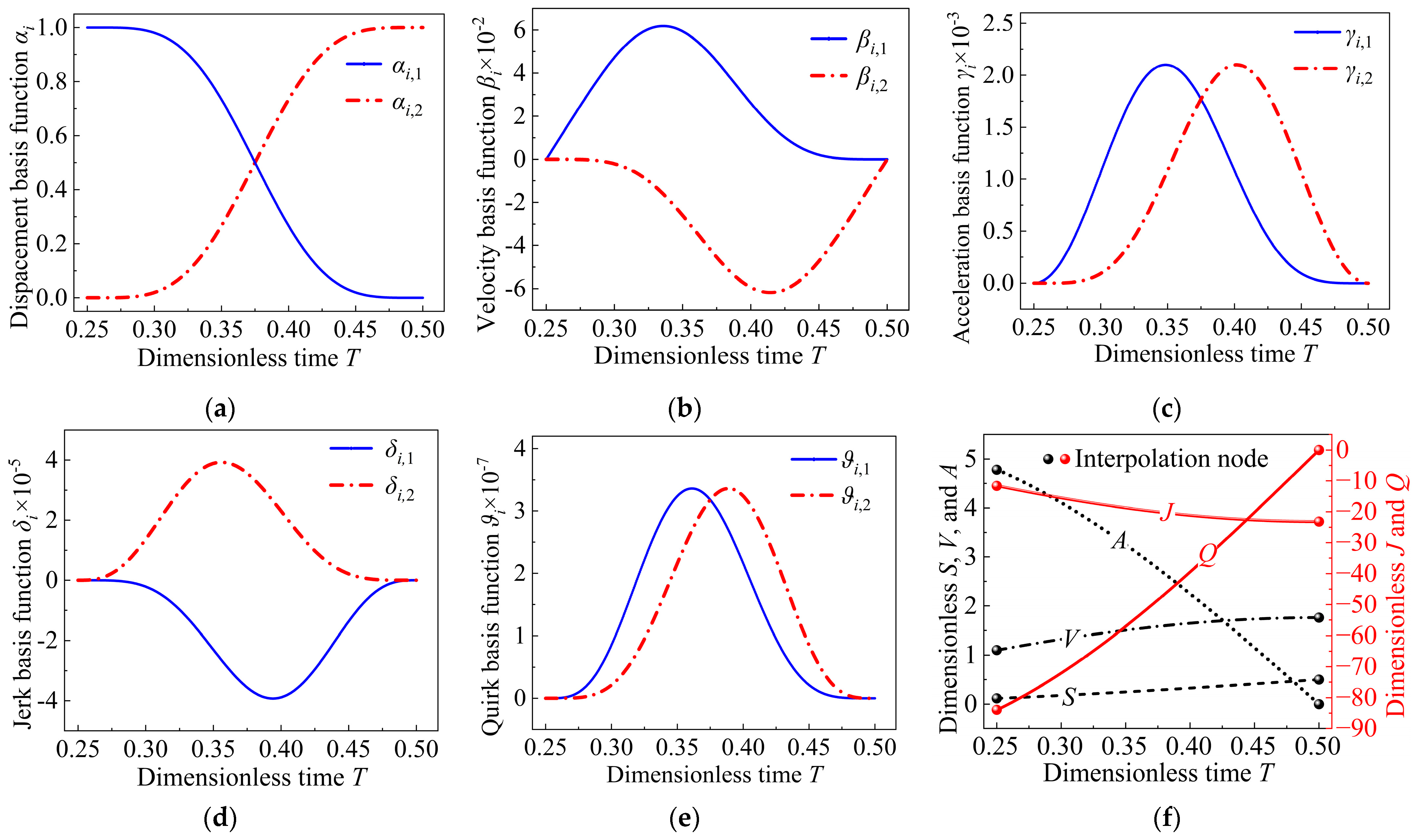
It is important to note that such explicit basis functions will contribute to enhanced interpolation efficiency as compared with previous implicit basis functions [7]. Similarly, the explicit analytical forms of basis functions in arbitrary time subintervals can be determined by solving the corresponding linear equation groups. Specifically, when provided with two sets of four-order motion data (

Table 1. Four-order motion data in the closed-time subinterval [0.25, 0.50].

T	S	V	A	J	Q
0.25	0.12	1.10	4.79	−11.58	−84.00
0.50	0.50	1.76	0	−23.16	0

) in the closed-time subinterval [0.25, 0.50], ten explicit basis functions and five interpolated splines can be determined using Equations (2)–(5), which are plotted in Figure 2.

Clearly, each basis function curve shows no abrupt changes, corners, or local oscillations, which are prerequisites for the creation of a smooth spline. Benefiting from this smooth nature, the interpolated displacement spline reaches C⁴ continuity in the closed-time subinterval [0.25, 0.50]. Furthermore, it can be inferred that when the motion data are single-valued (continuous) at each time point, a C⁴-continuous piecewise motion curve across the entire time interval can be synthesized by sequentially stitching the interpolated C⁴ spline in each subinterval.

3. Shape-Preserving Interpolation of High-Order Motion Curves

3.1. High-Order Interpolation Capability

To demonstrate the interpolation capability of the C4SI, the data-driven reconstruction of the typical MS motion curve, S_MS(T), is performed. Through the uniform sampling of the MS curve (Equation (10)) and its derived curves, four-order motion data at 81 dimensionless time points are extracted, which are taken as the raw discrete dataset for interpolation.

$$S_{\mathrm{MS}}(T)=\{\begin{array}{l}\frac{1}{\mathsf{\pi } + 4}\left(\mathsf{\pi }T-\frac{1}{4}\sin \left(4\mathsf{\pi }T\right)\right),\hspace{0.17em}\hspace{0.17em}\hspace{0.17em}\hspace{0.17em}\hspace{0.17em}\hspace{0.17em}\hspace{0.17em}\hspace{0.17em}\hspace{0.17em}\hspace{0.17em}\hspace{0.17em}\hspace{0.17em}\hspace{0.17em}T\in [0, 1/8)\\ \frac{1}{\mathsf{\pi } + 4}\left(\mathsf{\pi }T-\frac{9}{4}\sin \left(\frac{\mathsf{\pi } + 4\mathsf{\pi }T}{3}\right)+2\right),\hspace{0.17em}\hspace{0.17em}T\in [1/8, 7/8)\\ \frac{1}{\mathsf{\pi } + 4}\left(\mathsf{\pi }T-\frac{1}{4}\sin \left(4\mathsf{\pi }T\right)+4\right),\hspace{0.17em}\hspace{0.17em}\hspace{0.17em}\hspace{0.17em}\hspace{0.17em}\hspace{0.17em}\hspace{0.17em}\hspace{0.17em}T\in \left[7/8, 1\right]\hspace{0.17em}\end{array},$$

(10)

Since the continuous interpolation of multiple points is prone to high-degree oscillations (Runge’s phenomenon) [18], three different piecewise interpolants are adopted to interpolate the extracted discrete motion data, and the interpolated motion curves are plotted in Figure 3a−d. It was found that with 81 interpolation points, the piecewise linear interpolant (PLI) could reconstruct the basic S(T) curve but led to observable distortions in V(T) and severe oscillations in A(T). The piecewise Hermite interpolant (PHI) applies to the accurate reconstruction of S(T) and V(T) but suffers from pronounced oscillations in A(T). By contrast, the proposed C4SI could accurately reconstruct not only the basic S(T), V(T), and A(T) curves, but also the higher-order motion curves, including J(T) and Q(T). These results demonstrate the unique capability of the C4SI to reconstruct a shape-preserved, oscillation-free motion curve fulfilling the prespecified multiorder constraints (up to the fourth order), which cannot be achieved using conventional low-order piecewise interpolants.

3.2. Interpolation Accuracy and Error Convergence

To evaluate the accuracy of interpolation, the global root mean square error (RMSE) of displacement can be taken as a quantitative measure. This error can be calculated by comparing the interpolated motion curve f_n(T) with the reference motion curve f_ref(T) using the following equation:

$$\mathrm{RMSE}=\sqrt{\frac{1}{n_{\mathrm{R}}}{\displaystyle \sum _{i=1}^{n_{\mathrm{R}}}{\left(f_n\left[\left(i-1\right)\Delta T\right]-f_{\mathrm{ref}}\left[\left(i-1\right)\Delta T\right]\right)}^2}},$$

(11)

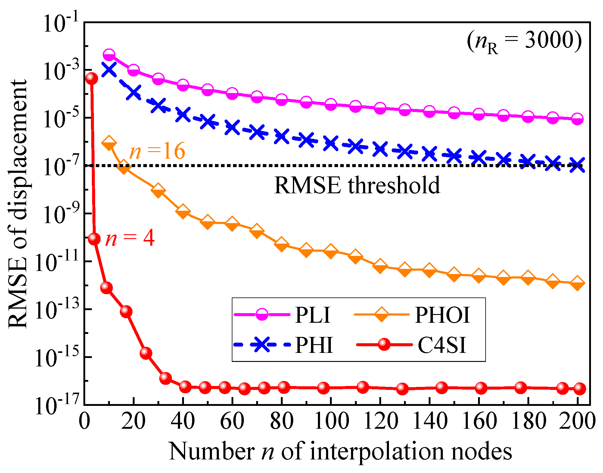
Here, the number (n_R) of the resampled points is well above the number (n) of the interpolated points. Using Equation (11), the RMSEs of four different piecewise interpolants, i.e., the conventional PLI and PHI [12], the latest PHOI [14], and the proposed C4SI in this study, are calculated, shown in Figure 4. Overall, the RMSEs of all the interpolants exhibit a common decreasing trend as the number of interpolated points increases, which is consistent with the trend in Ref. [12]. Meanwhile, the highest RMSE level is observed in the PLI (where no derivative is considered), while the lowest RMSE level is achieved using the C4SI (where four-order derivatives are considered). This result indicates that the achievable interpolation accuracy can be enhanced by increasing the order of the interpolated motion parameters.

It is also noted from Figure 3 that the C4SI achieves the specified RMSE threshold (10⁻⁷) with only four interpolated points (n = 4), whereas slightly more points (n = 16) are required for the PHOI and many more points (n > 190) are required for either the PHI or PLI. Notably, the RMSE of the C4SI rapidly converges to an ultra-low level of <10⁻¹⁶ within 41 interpolated points. These RMSE differences fully demonstrate the excellent interpolation accuracy and rapid error convergence of the C4SI.

4. Shape-Tuning for Kinematics and Dynamics Optimization

For the modification and optimization of the interpolated motion curves for high-speed applications, C4SI-based local tuning, global kinematics optimization, and global dynamics optimization strategies are proposed in this section and are validated with detailed numerical cases.

4.1. C4SI-Based Kinematics Optimization

4.1.1. Local Tuning for Improved Motion Continuity

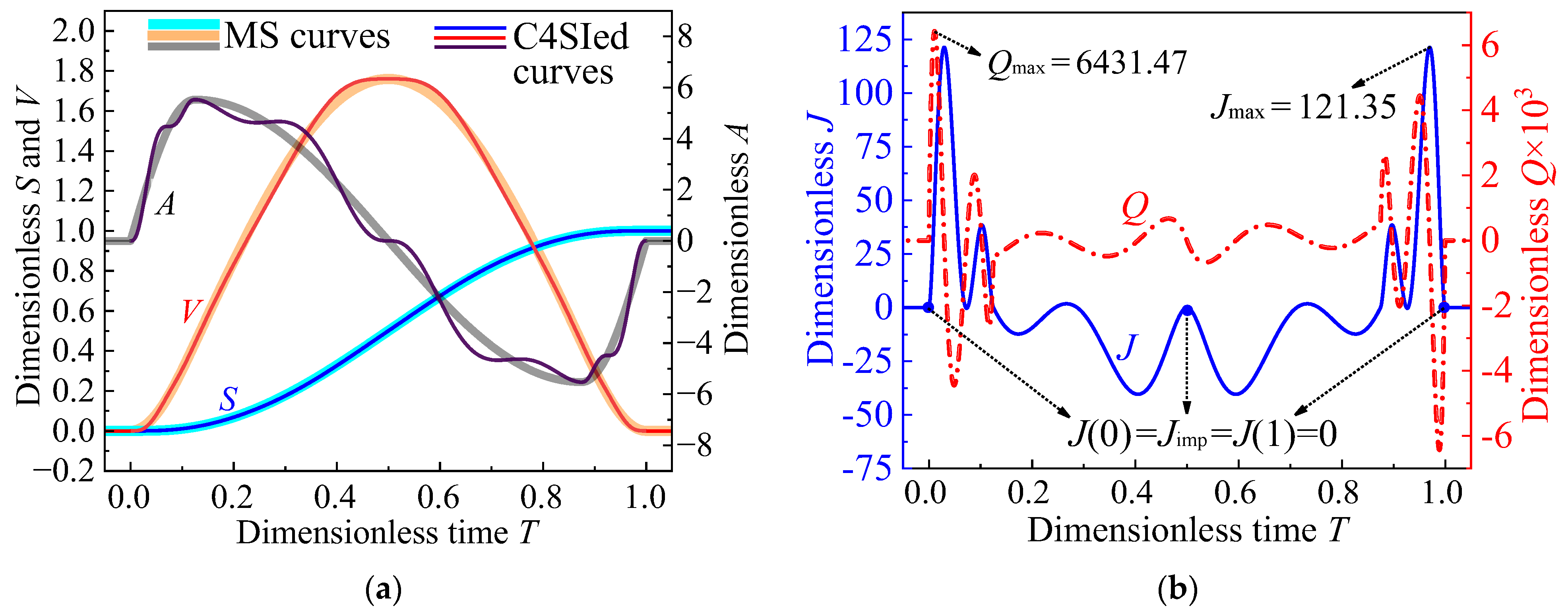
As aforementioned, there are mathematical defects in many standard motion curves. Specifically, for the typical MS curve (Figure 3), jerk jumps (J_jump = 69.47) are observed at T = 0 and 1, quirk jumps (Q_jump = 775.95) are observed at T = 0.125 and 0.875, and a large absolute jerk |J_imp| = 23.16 is observed at the crossover point T = 0.5, as listed in

Table 2. Raw motion data of the modified sine (MS) curve.

T	S	V	A	J	Q
0	0	0	0	0 (left); 69.47 (right)	0
0.125	0.02	0.44	5.53 (Amax)	0	−872.94 (left); −96.99 (right)
0.500	0.50	1.76 (Vmax)	0	−23.16 (Jimp)	0
0.875	0.98	0.44	−5.53 (−Amax)	0	96.99 (left); 872.94 (right)
1.000	1.00	0	0	69.47 (left); 0 (right)	0

. Such defects can potentially induce pronounced motion impacts to high-speed transmission systems [5,14].

Here, to improve the motion continuity, J(0) and J(1) are directly reassigned as 0, and Q(0.125) and Q(0.875) are reassigned as the mean values of the corresponding left and right limits. Meanwhile, to minimize the crossover impact (directly proportional to |J_imp|^1/3 [5]), the jerk value J_imp at T = 0.5 is reassigned as 0. Hence, the updated four-order motion data are obtained, as shown in

Table 3. Locally tuned motion data for improved motion continuity and reduced crossover impact.

T	S	V	A	J	Q
0	0	0	0	69.47 → 0	0
0.125	0.02	0.44	5.53	0	(−872.94 − 96.99)/2
0.500	0.50	1.76	0	−23.16 → 0	0
0.875	0.98	0.44	−5.53	0	(872.94 + 96.99)/2
1.000	1.00	0	0	69.47 → 0	0

. Then, through the C4SI of these locally tuned motion data, a new four-order motion curve is reconstructed, as plotted in Figure 5. As indicated, the interpolated motion curves are all continuous throughout the time interval, demonstrating the ultra-smooth feature (C⁴ continuity) of the reconstructed motion curve. Meanwhile, the absolute value of jerk |J_imp| at T = 0.5 is reduced to 0, which contributes to minimized crossover impacts in shape-locked indexing cam mechanisms [5]. Nevertheless, large jerk and quirk peaks are observed in Figure 5b, which are not desirable in high-speed scenarios. This result indicates that improving the continuity of motion does not necessarily imply better kinematic characteristics. Actually, as suggested by Ref. [19], considering high-order continuity may introduce additional equality (rigid) constraints, resulting in the decreased adaptability of the motion curves and increased motion peaks at unconstrained points. Therefore, the key to achieving better kinematic characteristics lies in the global optimal tuning of the high-order motion parameters, which will be demonstrated in the next subsection.

4.1.2. Global Kinematics Optimization for Minimized Motion Peaks

The kinematic optimization of the motion curve is a min–max problem involving the minimization of the maximum absolute motion characteristic value, where the global motion peak of primary concern is typically taken as the objective function [7,14]. However, in case-specific applications where the motion curves are complex functions involving undetermined parameters, it would be challenging to derive the analytical expression of the target motion peak, resulting in considerable difficulties in evaluating the objective function.

To address the above challenge, this study proposes a facile C4SI-based global kinematics optimization strategy based on the definite integral relations between the motion peaks and the derived motion functions. Specifically, for the typical MS curve (Figure 3), the definite integral relation between the displacement peak S_max and the velocity function V(T) can be determined as the following:

$$S_{\max }={\displaystyle {\int }_0^{1}V(T)\mathrm{d}T}=1,$$

(12)

That is, the displacement peak S_max can be determined using the area between the velocity function V(T) and the time coordinate T. Evidently, this relation applies to almost arbitrary non-dimensionalized motion curves [6], where the displacement functions increase monotonically from 0 to 1 as T rises from 0 to 1. Similarly, the definite integral relation between the velocity peak V_max and the acceleration function A(T) of the MS curve in Figure 3 can be determined as the following:

$$V_{\max }={\displaystyle {\int }_0^{T_{AE}}A(T)\mathrm{d}T,\hspace{0.17em}}(A\ge 0)\hspace{0.17em}\hspace{0.17em}\mathrm{or}\hspace{0.17em}\hspace{0.17em}{V}_{\max }={\displaystyle {\int }_{T_{AE}}^1\left|A(T)\right|\mathrm{d}T,\hspace{0.17em}}(A<0),$$

(13)

where T_AE = 0.5 is the only extreme point at which the acceleration function A(T) = 0.

Using Equation (13), the integral expression of the velocity peak V_max in the entire time interval [0, 1] can be derived as the following:

$$V_{\max }=\frac{1}{2}\left({\displaystyle {\int }_0^{T_{AE}}A(T)\mathrm{d}T\hspace{0.17em}}+{\displaystyle {\int }_{T_{AE}}^1\left|A(T)\right|\mathrm{d}T}\right)=\frac{1}{2}{\displaystyle {\int }_0^1\left|A(T)\right|\mathrm{d}T\hspace{0.17em}},$$

(14)

Notably, Equation (14) also applies to most of the motion curves (e.g., MS, MT, and MCV), with only one velocity peak in the time interval [0, 1]. Further, the definite integral relation between the acceleration peak A_max and the jerk function J(T) of the MS curve in Figure 3 can be derived as the following:

$$\begin{array}{l}{A}_{\max }={\displaystyle {\int }_0^{T_{JE1}}J(T)\mathrm{d}T=}{\displaystyle {\int }_{T_{JE1}}^{0.5}\left|J(T)\right|\mathrm{d}T}={\displaystyle {\int }_{0.5}^{T_{JE2}}\left|J(T)\right|\mathrm{d}T=}{\displaystyle {\int }_{T_{JE2}}^{1}J(T)\mathrm{d}T};\\ \Rightarrow A_{\max }=\frac{1}{4}{\displaystyle {\int }_0^1\left|J(T)\right|\mathrm{d}T}\end{array},$$

(15)

where T_JE1 = 0.125 and T_JE2 = 0.875 are the two extreme points at which the jerk function J(T) = 0. Note that in addition to the MS curve, Equation (15) also applies to typical symmetrical motion curves (e.g., MT, MCV, and standard quintic polynomials) with two opposite acceleration peaks in the entire time interval.

The applicability of the above definite integral relations in a variety of typical motion curves [20] are summarized in

Table 4. Applicability of definite integral relations in typical motion curves.

Definite Integral Relations	MS	MT	MCV	Cycloid Curve	Standard Quintic Polynomial	Asymmetrical Motion Curves
Equation (12)	✓	✓	✓	✓	✓	✓
Equation (14)	✓	✓	✓	✓	✓	✓
Equation (15)	✓	✓	✓	✓	✓	Partially applicable

. Based on its overall applicability, either Equation (14) or Equation (15) can be adopted as the candidate objective function for kinematics optimization. Furthermore, since the derived motion functions (such as A(T) and J(T)) are integrable (see Equations (2) and (3)), their definite integrals can be free of the time variable T and its power terms (e.g., T², T³, …). That is, either V_max or A_max (the candidate objective function) can be taken as the linear combination of the nodal motion parameters. These relations transform the complex time-varying non-linear kinematics optimization problem (min–max problem) into a route time-free linear programming problem, which can be handily resolved using conventional simplex or interior point methods.

To validate the proposed strategy, the global kinematics optimization of the reference motion curve (MS curve) is performed. Due to the good smoothness of the MS curve, it is difficult to achieve a simultaneous reduction in its multiple motion peaks [7]. As such, the integral expression of the acceleration peak A_max (Equation (15)), for instance, is defined as the primary objective function, which leads to the following global kinematics optimization model:

$$\mathrm{Min}:\hspace{0.17em}{A}_{\max }(S_i,\hspace{0.17em}{V}_i,\hspace{0.17em}{A}_i,\hspace{0.17em}{J}_i,\hspace{0.17em}{Q}_i)=\frac{1}{4}{\displaystyle {\int }_0^1\left|J(T;\hspace{0.17em}{S}_i,\hspace{0.17em}{V}_i,\hspace{0.17em}{A}_i,\hspace{0.17em}{J}_i,\hspace{0.17em}{Q}_i)\right|\mathrm{d}T},$$

(16)

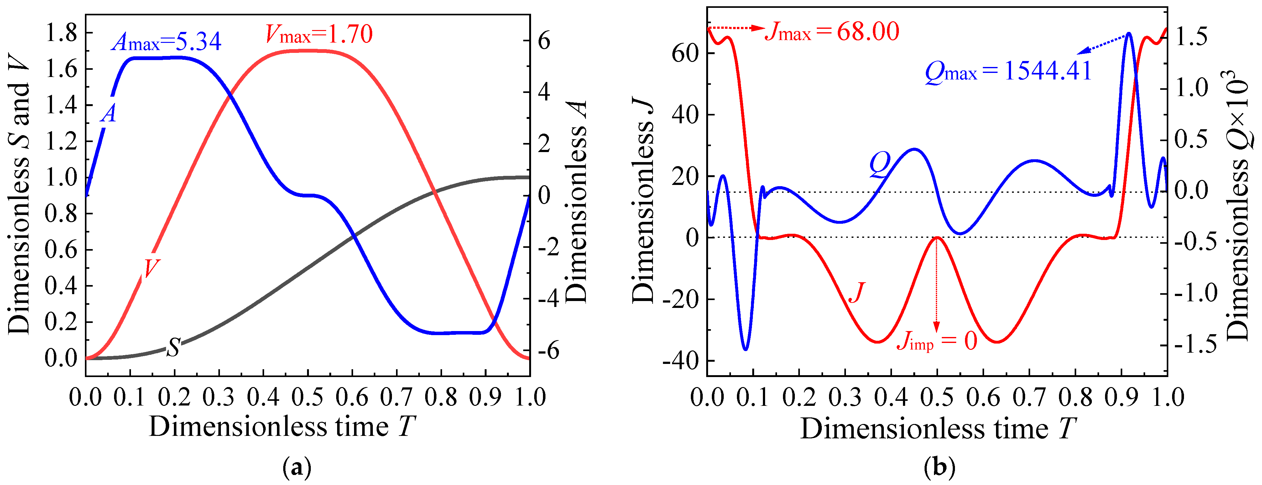
In Equation (16), the displacement parameters S_i are fixed to retain the basic positioning requirements, while the higher-order motion parameters (V_i, A_i, J_i, and Q_i) are allowed to be adjusted, in whole or in part, for kinematics optimization. The raw four-order motion parameters for global kinematics optimization are listed in

Table 5. Four-order motion parameters for global kinematics optimization.

T	S	V	A	J	Q
0	0	0	0	69.47 (Jmax) → 68.00	0
0.125	0.02	0.44	5.53 (Amax) → A2	0	Q2
0.500	0.50	1.76 (Vmax) → 1.70	0	−23.16 (Jimp) → 0	0
0.875	0.98	0.44	−5.53 (−Amax) → −A2	0	−Q2
1.000	1.00	0	0	69.47 (Jmax) → 68.00	0

. Note that the velocity and jerk peaks are, respectively, specified as V_max = 1.70 and J_max = 68.00, both of which are smaller than the original peaks.

Through the C4SI of the motion parameters (including both variables and constants) in Table 5, a flexible four-order motion curve can be created. Then, through the global kinematics optimization of the flexible motion curve using Equation (16), the optimal motion parameters can be determined. Finally, through the re-C4SI of the optimized motion parameters, an optimal four-order motion curve is obtained, shown in Figure 6. As indicated, the motion characteristic values of the optimized motion curve are V_max = 1.70, A_max = 5.33, J_max = J_jump = 68.00, |J_imp| = 0, and Q_jump = 0, which are all smaller than those of the original MS curve (

Table 6. Motion characteristic values of the reference and optimized motion curves (where “↓” signifies a decrease).

Motion Curves	Vmax	Amax	Jmax (Jjump)	|Jimp|	Qjump
Original MS curve (reference)	1.76	5.53	69.47	23.16	775.95
After C4SI-based global kinematics optimization	1.70 ↓	5.34 ↓	68.00 ↓	0 ↓	0 ↓

). This simultaneous reduction in five motion characteristic values represents a significant kinematics improvement in the MS curve, which is a challenging task for conventional kinematics optimization methods [7,14]. Based on these optimization outcomes, the feasibility and effectiveness of the proposed global kinematics optimization strategy were confirmed.

4.2. C4SI-Based Dynamics Optimization

4.2.1. Global Dynamics Optimization Model

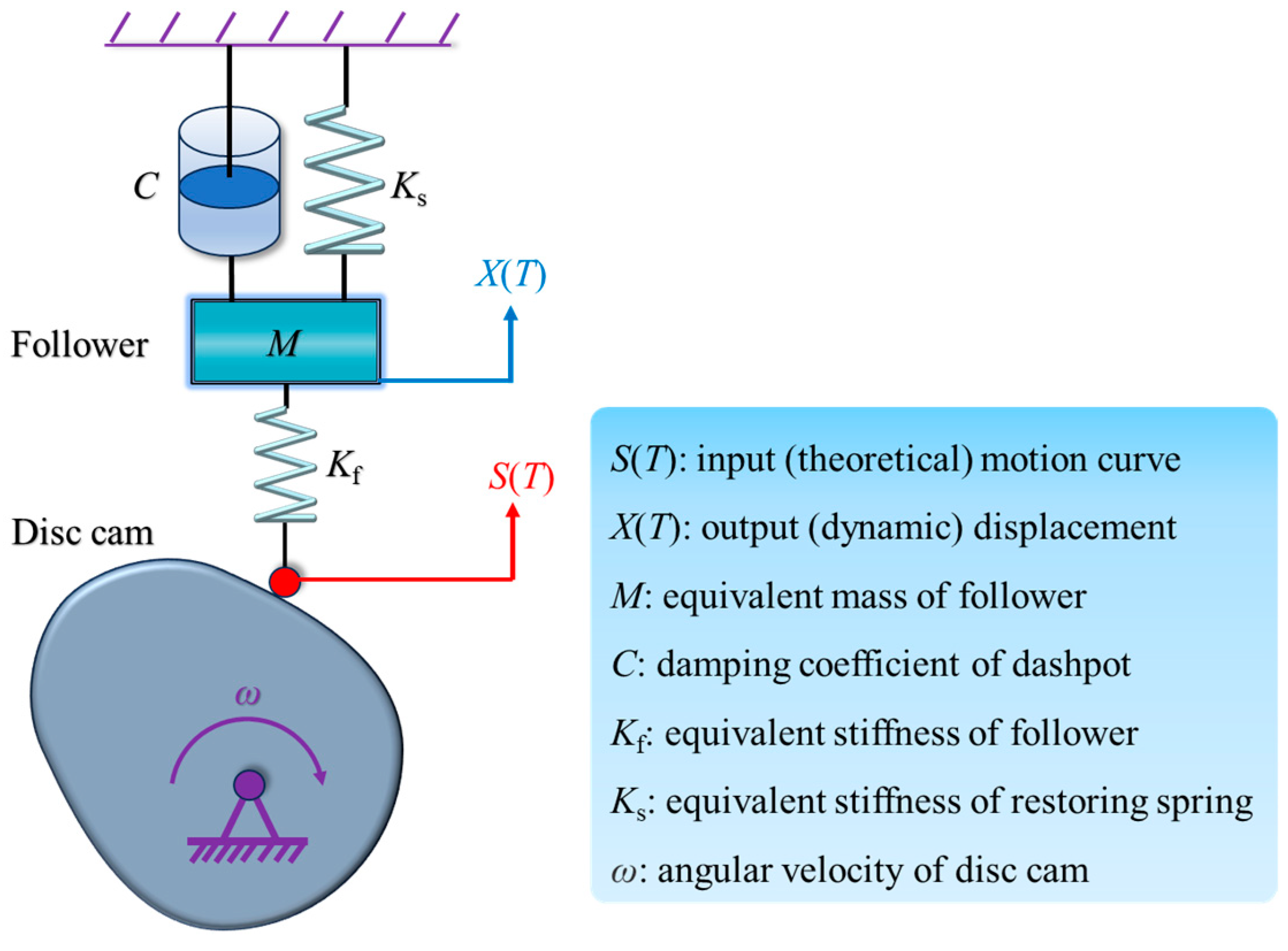
Dynamics characteristics are of major concern in cam-driven mechanical systems [21], particularly in high-speed scenarios [22]. Concerning the dynamics optimization of the motion curve, a typical disk cam-translating follower transmission system with a single degree of freedom (SDOF) is considered, as illustrated in Figure 7. To evaluate the theoretical contribution of the input motion curve (displacement excitation) independently, external disturbances such as force excitation or interface friction are not taken into consideration. This kind of SDOF model (Figure 7) has demonstrated its applicability in the dynamics representation of many high-speed industrial cam mechanisms [22,23].

The differential equation of motion of this SDOF model can be described as the following [24]:

$$\begin{array}{l}\frac{{\mathrm{d}}^{2}X(T)}{\mathrm{d}{T}^2}+4\mathsf{\pi }\xi \tau \frac{\mathrm{d}X(T)}{\mathrm{d}T}+{(2\mathsf{\pi }\tau )}^{2}X(T)={(2\mathsf{\pi }\tau )}^{2}S(T)\\ \mathrm{where} \xi =\frac{C}{2\sqrt{M(K_1 + K_2)}}\hspace{0.17em},\hspace{0.17em}\hspace{0.17em}\tau =\frac{\sqrt{(K_1 + K_2)/M}}{2\mathsf{\pi }/t_h}\hspace{0.17em}\end{array},$$

(17)

where t_h is the total rising time.

Considering an undamped dynamics system, a low level of damping ratio, ζ = 0.05, is specified for all optimization cases, while the period ratio τ, as a key indicator of the system’s running speed, varies from case to case. For high-speed cases, 0 < τ ≤ 6 is generally considered [14].

Here, the primary task is to minimize the absolute dynamic error |ε_d(T)| = |X(T) − S(T)| between the input motion curve S(T) and the output displacement X(T). However, in engineering practice where the input motion curve S(T) is a complex function, it is rather difficult to obtain the analytical solution X(T) of Equation (17) [14], let alone the analytical form of the dynamics objective function |ε_d(T)|. To circumvent this difficulty, the following integral objection function F with four weighting factors is suggested for global dynamics optimization:

$$\mathrm{Min}:F(S_i,\hspace{0.17em}{V}_i,A_i,\hspace{0.17em}{J}_i,\hspace{0.17em}{Q}_i)=w_V{\displaystyle {\int }_0^{1}V{(T)}^2\mathrm{d}T + }{w}_A{\displaystyle {\int }_0^{1}A{(T)}^2\mathrm{d}T + }{w}_J{\displaystyle {\int }_0^{1}J{(T)}^2\mathrm{d}T}+w_Q{\displaystyle {\int }_0^{1}Q{(T)}^2\mathrm{d}T},$$

(18)

where w_V, w_A, w_J, and w_Q are the velocity, acceleration, jerk, and quirk weighting factors, respectively.

The applicability of this kind of integral objection function in global dynamics optimization has been validated in previous studies [14,15]. However, differing from previous studies, the contribution of the fourth-order motion parameter (Q) is incorporated for the first time into the integral objective function F for better control of global dynamics characteristics. To balance the contribution of each integral term in Equation (18), the weighting factors are herein scaled by the squared motion peaks (see Table 2) of the reference curve (MS curve), i.e., w_V = $1/V_{\max }^2$, w_A = $1/A_{\max }^2$, w_J = $1/J_{\max }^2$, and w_Q = $1/Q_{\max }^2$. It is important to note that as with Equation (16), the integral objective function F in Equation (18) excludes the time variable T and its power terms, which contributes to enhanced computational feasibility and efficiency.

4.2.2. Effects of the Interpolation Point Number and Interpolation Order

As indicated in Equation (18), global dynamics optimization involves the optimal tuning of multiorder motion parameters at multiple time points. It is thus important to investigate the effects of the number of interpolated points and the highest order of interpolated motion parameters on the global dynamics optimization results.

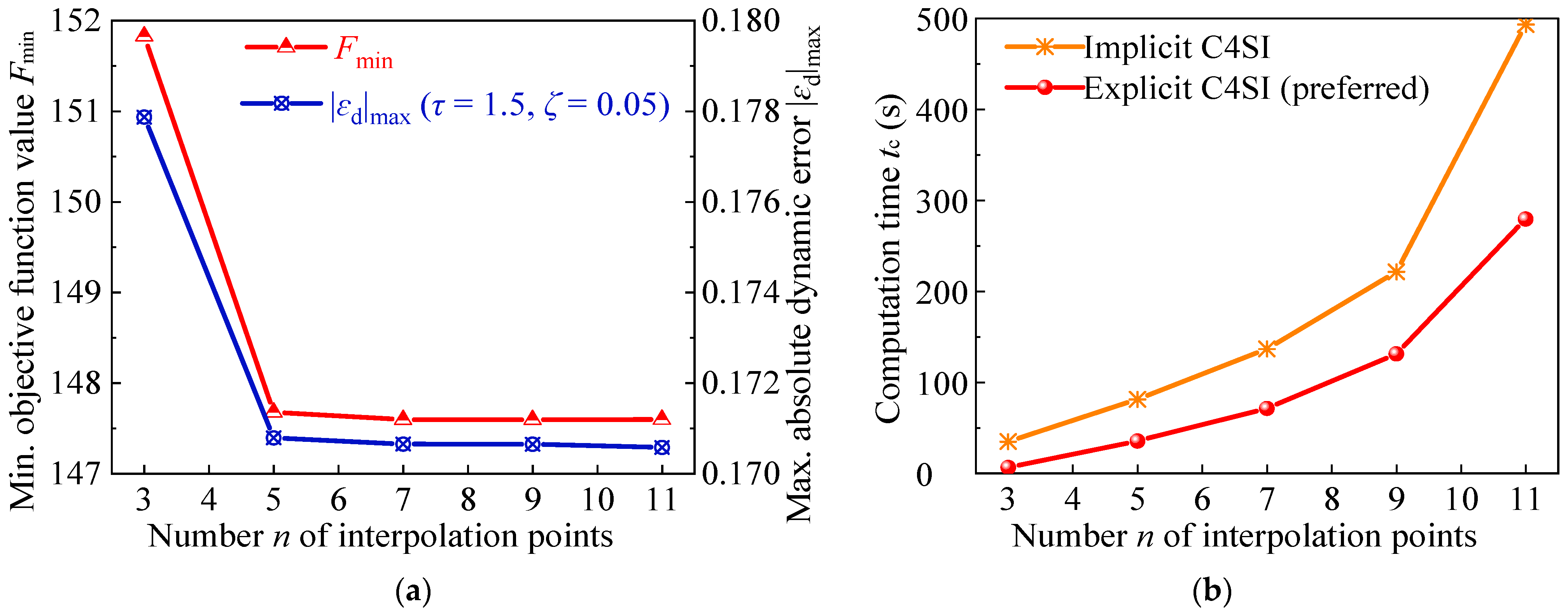
To address the first issue, the number n of interpolation points is specified as 3 to 11, while the order of motion parameters is fixed as C = 4. As illustrative examples, the specified four-order motion parameters in the cases of n = 3 and 5 are, respectively, listed in

Table 7. Four-order motion parameters in the case of three interpolation points (n = 3).

T	S	V	A	J	Q
0	0	0	0	J1	0
0.5	S2	V2	A2	J2	Q2
1.0	1.0	0	0	J3	0

and

Table 8. Four-order motion parameters in the case of five interpolation points (n = 5).

T	S	V	A	J	Q
0	0	0	0	J1	0
0.25	S2	V2	A2	J2	Q2
0.50	S3	V3	A3	J3	Q3
0.75	S4	V4	A4	J4	Q4
1.00	1.0	0	0	J5	0

. Through the C4SI combined with global dynamics optimization (Equation (18)), the minimum objective function value F_min and the optimal motion parameters in each case can be determined, which leads to the optimal high-speed motion curve S(T). Then, by utilizing the standard fourth-fifth order Runge-Kutta solver [14], Equation (17) can be solved numerically to obtain the numerical solution X(T_i), and hence the maximum absolute dynamic error |ε_d|_max. Figure 8a shows the calculated F_min in the cases of n = 3 to 11 and the associated |ε_d|_max of an undamped high-speed dynamics system (e.g., τ = 1.3, ζ = 0.05). Overall, both F_min and |ε_d|_max exhibit a decreasing trend as n rises, but the rate of decrease slows down as n > 5. Meanwhile, the computation time shows a pronounced increase as n rises (Figure 8b). In this regard, the preferred number of interpolated points for global dynamics optimization is determined as n = 5. It is important to note that compared with the implicit C4SI, the preferred explicit C4SI in Section 2.2 offers a significant reduction in computation time (Figure 8b), which demonstrates the good application potential of the proposed global dynamics optimization strategy.

To address the second issue, the highest order C of the considered motion parameters is specified as 2 to 4, while the number of interpolation points is fixed as n = 5. Through the C4SI combined with global dynamics optimization, the minimum objective function value F_min in each case and the associated maximum dynamic error |ε_d|_max are obtained, listed in

Table 9. Global dynamics optimization results in the cases of varied interpolation orders (where n = 5, τ = 1.3, ζ = 0.05).

Highest Order of Interpolated Motion Parameters C	Minimum Objective Function Value Fmin	Computation Time tc (s)	Optimized Motion Curve	Maximum Absolute Dynamic Error |εd|max
2	181.504	15.556	SII (T)	0.219
3	163.336	23.510	SIII (T)	0.200
4	147.677	35.567	SIV (T)	0.171

. Clearly, both F_min and |ε_d|_max decrease as the highest order of the interpolated motion parameter increases. This trend suggests that in comparison to merely controlling the low-order motion parameters, implementing full control of four-order motion parameters can yield more desirable dynamics characteristics. It can be further inferred that controlling higher-order (e.g., the fifth order) motion parameters may contribute to even lower dynamic error. Nevertheless, considering the pronounced increase in computational costs and the unclear physical significance of the fifth-order derivative, the preferred interpolation order is herein determined as C = 4.

Based on the above analyses, the optimized four-order motion curve in the case of n = 5 and C = 4, i.e., the S_IV(T) in Table 9, is selected as the target motion curve (displacement excitation) for the dynamics analyses. Using Equation (17), the dynamic displacements X(T) and dynamic errors ε_d(T) of the disc cam-translating follower system (Figure 7) within the high-speed range (τ ≤ 6) are calculated, shown in Figure 9. It can be found that within the considered period ratios, the system’s dynamic (output) displacements X(T) are in general consistency with the input motion curve S_IV(T) (Figure 9a), except when τ = 1, at which unwanted structural resonance occurs [14]. Notably, as τ ≥ 2, the transmission errors during the rise and return stages as well as the residual vibrations during the two dwell stages fall within 0.07 (Figure 9b), indicating a minor global dynamic error of <7%. These results suggest that the optimized four-order motion curve S_IV(T) in Table 9 can guarantee the desired dynamics characteristics and running stability across a wide range of high speeds.

4.2.3. Comparison of the Dynamics Responses

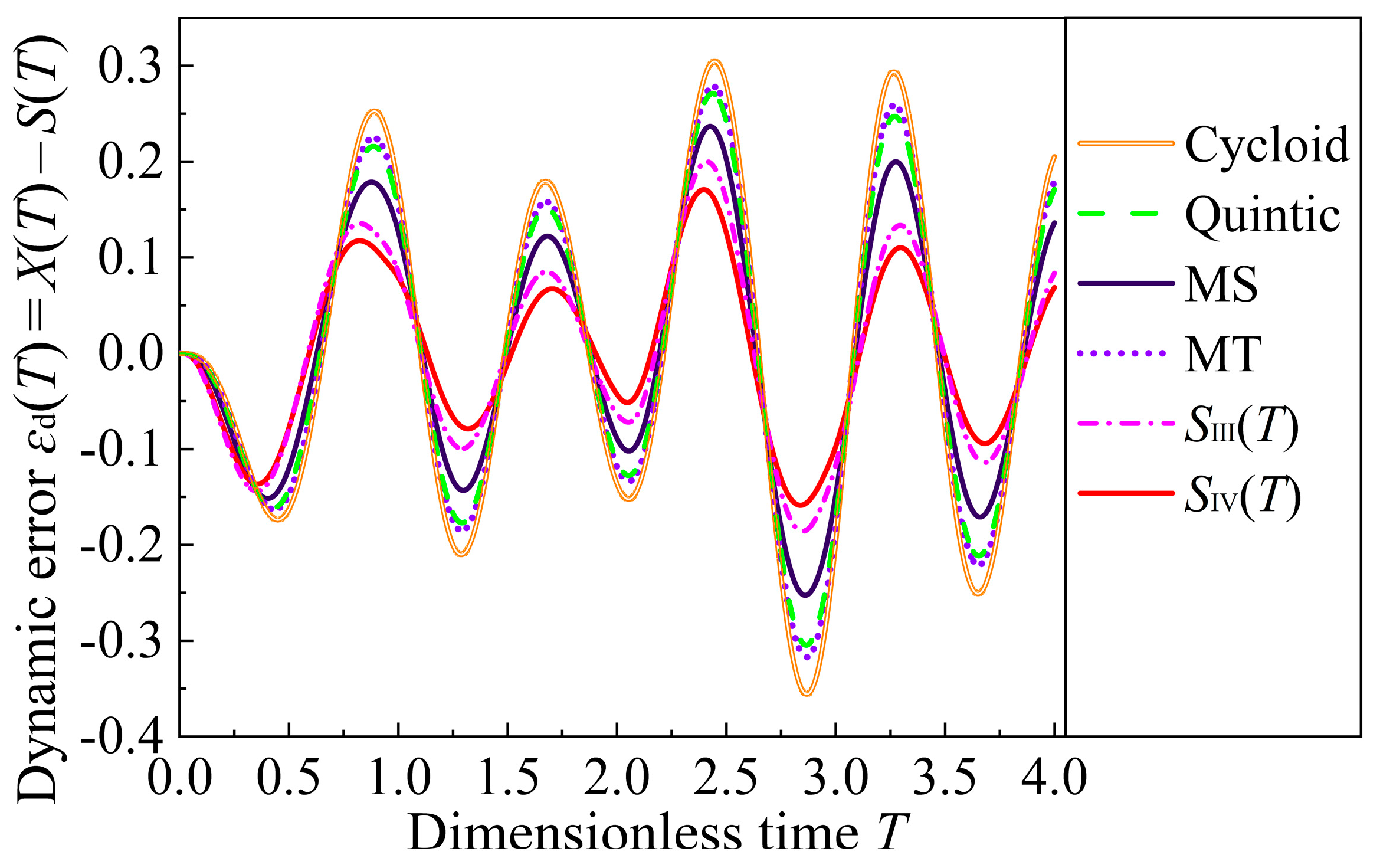
To comparatively evaluate the effectiveness of the C4SI-based global dynamics optimization strategy, the dynamic characteristics of the high-speed disc cam-translating follower system (τ = 1.3, ζ = 0.05) in response to different motion curves are calculated, as shown in Figure 10. Overall, compared with the standard motion curves (cycloid, quintic, MS, and MT) and the three-order motion curve S_III(T) in Table 9, the optimized four-order motion curve S_IV(T) yields the minimal high-speed transmission error and residual vibration over the whole rise-dwell-return-dwell cycle. This result, in combination with those in Figure 9, collectively demonstrate that C4SI-based global dynamics optimization offers an effective and general strategy for the optimal construction of four-order high-speed motion curves.

5. Discussions

This methodological study focuses on the mathematical modeling and computational optimization of the input motion curve, with the aim of achieving the active control of the output performance of a high-speed cam-follower system at the design level. To facilitate the implementation of the proposed C4SI and tuning strategies, it would be instructive to consider the following issues and discuss the potential solutions.

(1) Concurrent optimization: In the current study, kinematics optimization and dynamics optimization are conducted independently. For practical considerations, the concurrent optimal design of the motion curve considering both kinematic and dynamic characteristics is an important issue [25]. However, the kinematics and dynamics objective functions are often contradictory, particularly for high-speed cam mechanisms. Thus, to achieve the concurrent optimization of the follower’s motion curves, it is necessary to strike a balance between the kinematic and dynamic objectives.

(2) Model adaptability: As an interpolation-based model, the proposed C4SI is sensitive to the initial conditions and parameter variations. For cam motion design where the initial motion parameters are well-defined and vary within a limited range, this sensitivity is beneficial to capture the essential characteristics of the raw data. However, in some data-driven inverse design cases involving noise or outliers, the interpolated high-order curves may encounter overfitting or abnormal fluctuations. Thus, for extended applications such as inverse design, it is advisable to filter the raw dataset before proceeding with the C4SI and optimization.

(3) Computational efficiency: As the orders of the considered derivatives increase, it is natural that the number and highest degree of the basis functions will also increase, thereby leading to higher computational costs in the C4SI. For the offline optimal design of motion curves, this limitation is acceptable. Nevertheless, for online optimal design, the computational efficiency and robustness of the C4SI need to be further enhanced. In this regard, exploring more efficient and robust alternative basis functions for the C4SI, such as exponential or radial basis functions, is of particular interest. Meanwhile, since the interpolation splines within each subinterval are computed independently, parallel computing is highly recommended to enhance the interpolation efficiency.

(4) Cam manufacturing: Despite the detailed numerical demonstrations, the practical implementation of the proposed interpolation-tuning methodology still relies on the geometrical accuracy of the manufactured cam profile. In this regard, ultra-precision machine tools incorporating appropriate curve discretization strategies are essential for manufacturing an ideal cam that precisely conforms to the optimized motion curve.

6. Conclusions

The study introduces a powerful C⁴-spline interpolant (C4SI) and combines it with unique time-free global kinematics/dynamics optimization strategies for the optimal construction of advanced four-order motion curves for high-speed scenarios. The design and optimization of high-speed cam profiles are adopted as application cases utilized to validate the feasibility and effectiveness of the proposed interpolation and tuning strategies. The observations and implications of this study are outlined as follows:

(1)

Through utilizing the C4SI with the provided four-order motion data, a high-fidelity, divergence-free motion curve can be constructed. The global displacement error of the constructed motion curve falls below the specified threshold (10⁻⁷) with only four interpolation points and then rapidly converges to a minimal level (10⁻¹⁶). Such excellent interpolation accuracy and fast error convergence highlight the promising potential of the C4SI in reverse engineering applications involving high-order derivative constraints at massive discrete points.

(2)

Employing the C4SI for variable motion parameters facilitates the creation of a flexible and tunable motion curve with undetermined parameters. Through time-free global kinematics optimization, a simultaneous reduction in five motion characteristic values (V_max, A_max, J_max, |J_imp|, and Q_jump) is achieved. This reduction signifies significant kinematic enhancements for high-speed motion systems compared to the reference motion curves.

(3)

Through the C4SI-based global dynamics optimization of the motion parameters, an optimized four-order high-speed motion curve S_IV(T) can be achieved. Notably, S_IV(T) offers minimal high-speed transmission error and residual vibration throughout the whole motion cycle, which outperforms the standard motion curves and the three-order motion curve.

Beyond high-speed cam design, the proposed interpolation and tuning methodology may also be applicable to the computer-aided design of ultra-smooth surfaces [26], motion control of manipulators and robots [27], and high-order discretizations for finite element calculations [28]. These promising applications await exploration and implementation by researchers from various fields.

References

1. Zhang, Y.; Ji, S.; Zhao, J.; Xiang, L. Tolerance analysis and allocation of special machine tool for manufacturing globoidal cams. Int. J. Adv. Manuf. Technol. 2016, 87, 1597–1607. [Google Scholar] [CrossRef]
2. Shi, X.; Wang, K.; Li, G.; Lyu, C.; Zhao, L.; Chen, J.; Sun, L.; Wu, H. Study on temperature field uniformity of dynamic induction heating for camshaft of marine diesel engine. Machines 2024, 12, 215. [Google Scholar] [CrossRef]
3. Bäsel, U. Using the incomplete beta function as transfer function for dwell–rise–dwell motions. Mech. Mach. Theory 2023, 188, 105387. [Google Scholar] [CrossRef]
4. Flores, P. A computational approach for cam size optimization of disc cam-follower mechanisms with translating roller followers. J. Mech. Robot. 2013, 5, 041010. [Google Scholar] [CrossRef]
5. Zhou, C.J.; Hu, B.; Chen, S.Y.; Ma, L. Design and analysis of high-speed cam mechanism using Fourier series. Mech. Mach. Theory 2016, 104, 118–129. [Google Scholar] [CrossRef]
6. Norton, R.L. Cam Design and Manufacturing Handbook, 2nd ed.; Industrial Press Inc.: New York, NY, USA, 2002. [Google Scholar]
7. Yu, J.W.; Luo, H.; Hu, J.Z.; Nguyen, T.V.; Lu, Y.T. Reconstruction of high-speed cam curve based on high-order differential interpolation and shape adjustment. Appl. Math. Comput. 2019, 356, 272–281. [Google Scholar] [CrossRef]
8. Abderazek, H.; Yildiz, A.R.; Mirjalili, S. Comparison of recent optimization algorithms for design optimization of a cam-follower mechanism. Knowl.-Based Syst. 2020, 191, 105237. [Google Scholar] [CrossRef]
9. Nguyen, T.T.N.; Kurtenbach, S.; Husing, M.; Corves, B. A general framework for motion design of the follower in cam mechanisms by using non-uniform rational B-spline. Mech. Mach. Theory 2019, 137, 374–385. [Google Scholar] [CrossRef]
10. Qiu, H.; Lin, C.; Li, Z.; Ozaki, H.; Wang, J.; Yue, Y. A universal optimal approach to cam curve design and its applications. Mech. Mach. Theory 2005, 40, 669–692. [Google Scholar] [CrossRef]
11. Nguyen, V.; Kim, D. Flexible cam profile synthesis method using smoothing spline curves. Mech. Mach. Theory 2007, 42, 825–838. [Google Scholar] [CrossRef]
12. Borboni, A.; Aggogeri, F.; Elamvazuthi, I.; Incerti, G.; Magnani, P.L. Effects of profile interpolation in cam mechanisms. Mech. Mach. Theory 2020, 144, 103652. [Google Scholar] [CrossRef]
13. Jiang, J.K.; Iwai, Y.R.; Su, H. Minimizing and restricting vibrations in high-speed cam-follower systems over a range of speeds. J. Appl. Mech. 2007, 74, 1157–1164. [Google Scholar] [CrossRef]
14. Luo, H.; Yu, J.W.; Li, L.J.; Huang, K.F.; Zhang, Y.M.; Liao, K. A novel framework for high-speed cam curve synthesis: Piecewise high-order interpolation, pointwise scaling and piecewise modulation. Mech. Mach. Theory 2022, 167, 104477. [Google Scholar] [CrossRef]
15. Yu, J.W.; Huang, K.F.; Luo, H.; Wu, Y.; Long, X.B. Manipulate optimal high-order motion parameters to construct high-speed cam curve with optimized dynamic performance. Appl. Math. Comput. 2020, 371, 124953. [Google Scholar] [CrossRef]
16. Lu, Y.-S.; Lin, Y.-Y. Smooth motion control of rigid robotic manipulators with constraints on high-order kinematic variables. Mechatronics 2018, 49, 11–25. [Google Scholar] [CrossRef]
17. Han, X. Shape-preserving piecewise rational interpolation with higher order continuity. Appl. Math. Comput. 2018, 337, 1–13. [Google Scholar] [CrossRef]
18. Zhang, R.-J.; Ma, W. An efficient scheme for curve and surface construction based on a set of interpolatory basis functions. ACM Trans. Graph. 2011, 30, 1–11. [Google Scholar] [CrossRef]
19. Sun, Z.; Zhang, B.; Cheng, L.; Zhang, W. Application of the redundant servomotor approach to design of path generator with dynamic performance improvement. Mech. Mach. Theory 2011, 46, 1784–1795. [Google Scholar] [CrossRef]
20. Rothbart, H.A. Cam Design Handbook, 1st ed.; McGraw-Hill Professional: New York, NY, USA, 2004. [Google Scholar]
21. Merticaru, E.; Merticaru, V.; Nagîț, G.; Mihalache, A.M.; Tăbăcaru, L.L.; Rîpanu, M.I. Analytical, numerical and experimental analysis of a positive displacement cam mechanism—A case study. Machines 2023, 11, 770. [Google Scholar] [CrossRef]
22. Kaplan, H. Mathematical modeling and simulation of high-speed cam mechanisms to minimize residual vibrations. Proc. Inst. Mech. Eng. Part C J. Mech. Eng. Sci. 2014, 228, 2402–2415. [Google Scholar] [CrossRef]
23. Yousuf, L.S. Experimental and simulation investigation of nonlinear dynamic behavior of a polydyne cam and roller follower mechanism. Mech. Syst. Sig. Process. 2019, 116, 293–309. [Google Scholar] [CrossRef]
24. Chew, M.; Chuang, C.H. Minimizing residual vibrations in high-speed cam-follower systems over a range of speeds. J. Mech. Des. 1995, 117, 166–172. [Google Scholar] [CrossRef]
25. Bi, Z.M.; Zhang, W.-J. Concurrent optimal design of modular robotic configuration. J. Robot. Syst. 2001, 18, 77–87. [Google Scholar] [CrossRef]
26. Li, Y.; Zhao, X.; Ray, N.; Jiao, X. Compact feature-aware Hermite-style high-order surface reconstruction. Eng. Comput. 2021, 37, 187–210. [Google Scholar] [CrossRef]
27. Feng, M.; Dai, J.; Zhou, W.; Xu, H.; Wang, Z. Kinematics analysis and trajectory planning of 6-DOF hydraulic robotic arm in driving side pile. Machines 2024, 12, 191. [Google Scholar] [CrossRef]
28. Gravenkamp, H.; Saputra, A.A.; Duczek, S. High-order shape functions in the scaled boundary finite element method revisited. Arch. Comput. Methods Eng. 2021, 28, 473–494. [Google Scholar] [CrossRef]
Figure 1. (a) Schematic illustration of a typical disc cam-translating follower system, and (b) process steps for the optimal construction of four-order motion curves.
Machines 12 00283 g001
Figure 2. Representative basis functions for (a) displacement αi(T), (b) velocity βi(T), (c) acceleration γi(T), (d) jerk δi(T), and (e) quirk ϑi(T), and (f) the interpolated splines in the closed-time subinterval [0.25, 0.50].
Machines 12 00283 g002
Figure 3. (a) PLI, (b) PHI, and (c) C4SI reconstructed S(T), V(T), and A(T) curves. (d) C4SI-reconstructed J(T) and Q(T) curves. PLI: piecewise linear interpolant (PLI); PHI: piecewise Hermite interpolant; C4SI: C4-spline interpolant.
Machines 12 00283 g003
Figure 4. Root mean square errors (RMSEs) of the interpolated displacement curves using different piecewise interpolants.
Machines 12 00283 g004
Figure 5. Interpolated four-order motion curve using the C4SI of locally tuned motion data in Table 3: (a) displacement curve S(T), velocity curve V(T), and acceleration curve A(T), and (b) jerk curve J(T) and quirk curve Q(T).
Machines 12 00283 g005
Figure 6. Reconstructed motion curves after global kinematics optimization: (a) displacement S(T), velocity V(T), and acceleration A(T) curves, and (b) jerk J(T) and quirk Q(T) curves.
Machines 12 00283 g006
Figure 7. Typical high-speed disc cam-translating follower system with a single degree of freedom.
Machines 12 00283 g007
Figure 8. Global dynamics optimization results in cases with different numbers of interpolated points: (a) minimum objective function value Fmin and maximum absolute dynamic error |εd|max; (b) computation costs in cases using the implicit and explicit C4SI.
Machines 12 00283 g008
Figure 9. High-speed dynamics responses of the disc cam-translating follower system: (a) dynamic (output) displacement X(T) and (b) dynamic error εd(T) = X(T) − S(T).
Machines 12 00283 g009
Figure 10. Comparison of high-speed dynamics responses to different motion curves.
Machines 12 00283 g010