Graph Convolutional Network Based on CQT Spectrogram for Bearing Fault Diagnosis

Abstract

In this paper, a graph convolutional network is constructed and applied for bearing fault diagnosis. Specifically, the constant-Q transform (CQT) is first adopted for spectral analysis of vibration signals, where the frequencies are distributed in the logarithmic scale. Varied frequency resolutions can be obtained to satisfy the spectral resolution requirement and reduce signal dimension. Afterwards, the CQT spectrum is modeled by a graph, where nodes are frequency bins and edges reflect the inner relationship of different bins. There are edges between the fundamental and harmonic components. Then, a two-layer graph convolutional network (GCN) is utilized to assess the significance of vibration sources within the mixed signals. Finally, the bearing faults are determined according to the output of the GCN. To the best of our knowledge, this is the first work to model the vibration signal in this graph structure. The advantage of this approach lies in the simplification of edge definitions, facilitating shared connectivity relationships between the fundamental frequency and harmonics. Its performance was compared with another state-of-the-art fault diagnosis model. Experimental results demonstrate that the proposed model obtains higher accuracy, and it is more effective in extracting discriminative features.

1. Introduction

Rolling bearings play a crucial role in modern industry [1]. Bearing failures, predominantly attributed to wear [2] and fatigue cracking [3,4], significantly compromise equipment reliability and safety. Such malfunctions may precipitate grave accidents and operational halts. Hence, conducting regular inspections to detect early signs of bearing anomalies is pivotal for ensuring the steady and secure functioning of machinery.

Traditionally, fast Fourier transform (FFT) has been the foundation of vibration signal analysis in bearing fault diagnosis. Despite its widespread application, FFT is hampered by some limitations, such as its fixed frequency resolution, which may not capture the details of complex vibration signals, especially when fault characteristics are obscured by noise [5]. Additionally, conventional spectral analysis methods, with their linear frequency scales, may fall short in pinpointing the fundamental frequencies essential for accurate fault identification [6]. Moreover, there is a lot of redundant information in the higher-frequency range due to its constant frequency resolution.

To address the intricacies of fault diagnosis, a variety of advanced methodologies have been explored, enriching the diagnostic landscape. Among these, techniques such as the short-time Fourier transform (STFT), autogram, encurgram, IESFOgram, infogram, and curtogram stand out [7,8,9,10,11,12]. The autogram, for instance, is renowned for its adeptness in selecting optimal demodulation bands, showcasing remarkable efficacy in noisy environments and thus outperforming traditional kurtosis-based methods. In a similar vein, the encurgram presents an innovative multi-band demodulation strategy, which has proven its worth in both simulated and practical settings, effectively overcoming the challenges associated with narrowband methods in the face of wideband carrier signals prevalent in machinery.

Expanding on this mix of different methods, more sophisticated and adaptive diagnostic techniques have been developed, offering precise and flexible time–frequency analysis capabilities. Notably, the CQT and the STFT have been integrated within convolutional neural network (CNN)-based frameworks, enhancing sound classification and fault detection. Research, such as that conducted by Huzaifah [13], illustrates that while mel-scale STFT may exhibit marginal superiority in certain scenarios, a thorough evaluation indicates that techniques like CQT can attain higher classification accuracy. This is accomplished through a more precise detection of signal complexities, a critical aspect in situations where these fine details are crucial for identifying faults accurately.

Parallel advancements in bearing fault diagnosis have seen the successful incorporation of deep learning techniques, with studies by Zhang et al. [14], Neupane and Seok [15], and Hoang and Kang [16] highlighting the efficacy of convolutional neural networks, recurrent neural networks (RNNs), and support vector machines (SVMs), among others. Recently, an attention-embedded quadratic network was proposed, which intrinsically incorporates an attention mechanism in the network [17]. These approaches have shown promise in addressing the complex pattern recognition challenges inherent in bearing fault detection and classification.

Graph convolutional networks offer significant advantages in bearing fault diagnosis and classification due to their ability to process complex relational data. By leveraging the inherent structure of machinery data [18], GCNs excel in identifying complex patterns and relationships that traditional methods might miss [19]. This advanced analytical capability results in higher accuracy and efficiency in fault detection, making GCNs a powerful tool for maintaining the reliability and safety of industrial systems, thus revolutionizing the approach to bearing fault diagnostics.

Inspired by the advancements in the control of high-order uncertain nonlinear systems [20,21], a GCN is introduced in this work. Different from the previous ones, the graph is constructed according to the inner connection relationship of fundamental and harmonic components of vibration signals. To construct an adjacent matrix effectively and streamline the spectrum by eliminating extraneous details, CQT [22] is adopted for spectral analysis. Therefore, a graph is constructed in this work based on CQT spectral analysis for bearing fault diagnosis. The main contributions of this work include the following.

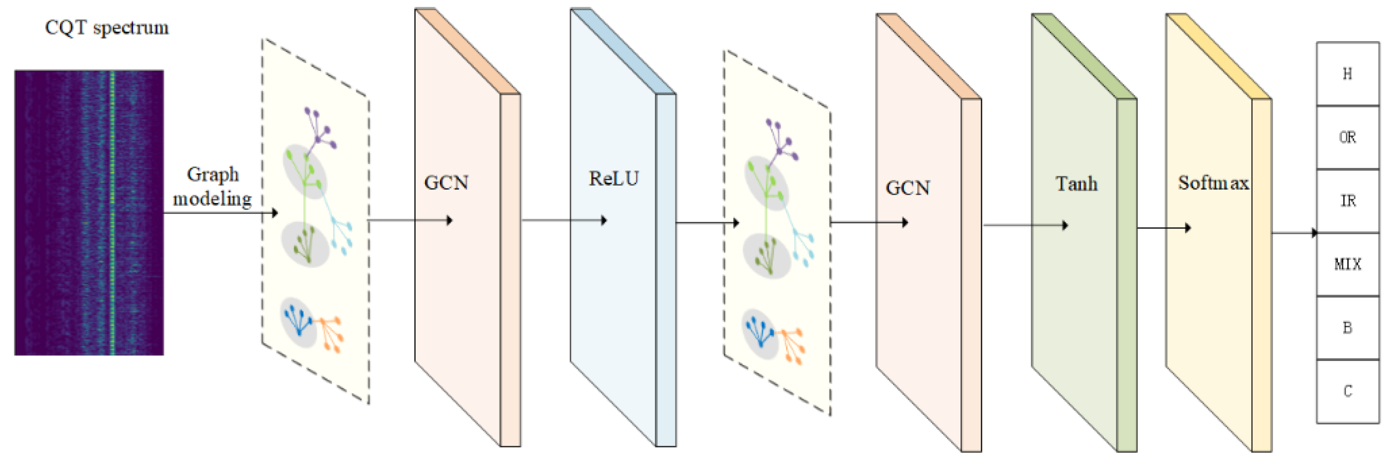
• Utilize CQT for spectral analysis: The paper applies CQT for spectral analysis of vibration signals into a logarithmic frequency scale. This transformation provides a variable frequency resolution for facilitating the graph modeling and remove redundant information.
• Innovatively model vibration signals as a graph structure: Unlike traditional methods that treat vibration signals linearly, this paper models these signals as graphs in the frequency domain. In this graph-based representation, nodes represent different frequency bins, while edges depict the harmonic relationships between these frequencies.
• Develop a GCN-based model for bearing fault diagnosis: A GCN is utilized to automatically learn the complex mapping function from CQT spectrum to fault categories. Experimental results demonstrate that the proposed approach is very effective.

The paper is organized as follows. Constant-Q transform and the graph convolutional network are introduced in Section 2. The proposed approach is elaborated upon in Section 3. The experimental results and discussions are provided in Section 4. Finally, the conclusions are drawn in Section 5.

2. Preliminary

2.1. Constant-Q Transform

CQT was introduced with a primary focus on its applications in music signal processing [22]. Originally designed for that purpose, the CQT provides a more precise representation of pitch information within audio signals. While conventional spectral representations may overlook harmonic structures associated with pitch, the CQT adeptly captures these features, resulting in more accurate pitch information.

Benefiting from its efficiency in capturing subtle frequency variations, CQT surpasses short-time Fourier transform (STFT) in extracting features related to signal frequency. Consequently, in various applications, CQT serves as a more effective and reliable analytical tool.

Given a signal $x(n)$, constant-Q transformation is defined as per [22]:

$${\mathrm{X}}^{cqt}(k)=\frac{1}{N_k}{\displaystyle \sum _{n=0}^{N_k-1}x}(n)w_{N_{\dot{k}}}(n)e^{-j2\pi nQ/N_{\dot{k}}}$$

(1)

where $k$ is the frequency index, $Nk$ is the length of the window function $w_{N_{\dot{k}}}(n)$ is the window function, and the quality factor (Q) is defined as per [22]:

$$Q=\frac{f_k}{{\delta }_{f_k}}$$

(2)

where $f_k$ represents the center frequency and ${\delta }_{f_k}$ represents the bandwidth at frequency $f_k$.

As illustrated in Equation (1), CQT differs from the traditional Fourier transform by adopting a constant Q (quality factor) frequency spacing. In CQT, the width of each frequency bin remains constant relative to frequency, unlike the evenly spaced bins in the Fourier transform. As a result, CQT exhibits nonlinear frequency resolution and high-resolution properties. This suggests that CQT can more precisely capture the frequency characteristics of signals.

2.2. Graph Convolutional Network

The GCN is widely used for processing non-Euclidean data by utilizing topological connections in a graph structure [23]. A GCN is essentially a neural network that performs matrix transformations to aggregate node information using edge information. This allows for automatic learning of node features and correlation information between nodes.

Existing models can be divided into two categories: spectral-based and spatial-based methods, depending on the type of graph. In the spectral-based method, the eigenvectors of the Laplace matrix undergo a Fourier transform to obtain a spectral filter shape. On the other hand, the spatial-based method directly convolves the nodes of the graph and their neighbors, isolating the rest of the graph and avoiding the negative effects of feature decomposition. This approach is easier to achieve and extend by simplifying the local node neighborhood.

This work follows the idea of the spatial-based perspective. Therefore, the GCN is considered from a spatial perspective. The input to the GCN consists of the feature vector associated with each node, which can be viewed as graph signals. The adjacent matrix $\mathbf{A}$ defines the total edges between the nodes. Finally, the output layer makes predictions based on the learned node embeddings, such as node classification or symbol labels. In summary, the GCN learns representations by aggregating and transforming node features across the graph environment.

An undirected connected graph $\mathcal{G}=(\mathcal{V},\mathcal{E},A)$ consists of a set of nodes $\mathcal{V}$ and a set of edges $\mathcal{E}$ that connect them. If there is an edge between node $i$ and node $j$ in a weight graph, the adjacent matrix $\tilde{A}$ is equal to the weight of this edge. Otherwise, $A(i,j)=0$. In an unweighted graph, if there is an edge between node $i$ and node $j$, then the adjacent matrix $A(i,j)=1$. The degree matrix $\tilde{D}$ of $\tilde{A}$ is diagonal with $\mathbf{D}(i,i)={\displaystyle \sum _{j=1}^N}\mathbf{A}(i,j)$ . The Laplacian matrix of $A$ is represented as $L=D-A$. Accordingly, the normalized graph Laplacian matrix $\tilde{L}$ is defined as per [23]:

$$\tilde{L}=I_N-D^{-\frac{1}{2}}A{D}^{-\frac{1}{2}}$$

(3)

A signal, depicted by a graph, can be succinctly captured as an M-dimensional vector $Y\in {ℝ}^{N\times M}$, where $Y(i)\in {ℝ}^M$ signifies the input feature at node $i$. A multi-layer GCN can be defined by the following layer-wise propagation rule [23]:

$$H^{(l+1)}=\sigma ({\tilde{D}}^{-\frac{1}{2}}\tilde{A}{\tilde{D}}^{-\frac{1}{2}}{H}^{(l)}{W}^{(l)})$$

(4)

where $\tilde{A}=A+I_N$ is an adjacent matrix with an added self-connected undirected graph that is equivalent to adding a self-loop to the original graph. The entire connection relations of the nodes are defined by an adjacent matrix $A\in {ℝ}^{N\times N}$, $I_N$ is the identity matrix of size $N\times N$, $W^{(l)}$ is a layer-specific trainable weight matrix, and $\sigma (\cdot )$ denotes an activation function, such as the $\mathrm{ReLU}(\cdot )=\max (0, \cdot )$. $H^{(l)}\in {ℝ}^{N\times D}$ is the matrix of activations in the $l\text{-}\mathrm{th}$ layer, and $H^{(0)}$ represents the input $Y$.

3. Proposed Approach

This paper proposes a fault diagnosis approach employing a GCN for the analysis of vibration signals, as illustrated in Figure 1. This approach incorporates CQT to represent spectral features of the vibration signals. Subsequently, the CQT spectrum is transformed into a graph structure to facilitate feature learning through the GCN. A two-layer GCN model is utilized to extract high-level features from the signals and identify the fault type. The study specifically addresses six common types of bearing faults: normal, inner race fault, outer race fault, ball fault, cage fault, and mixed faults. The proposed approach will be elaborated upon in detail in the following subsections.

3.1. Spectrum Modeling Using Graph

Benefit from GCNs’ efficiency in extracting features from non-Euclidean structured data with a reduced number of nodes, this paper leverages a GCN to realize effective bearing fault diagnosis. The input data is first transformed into a CQT spectrogram. Subsequently, the constructed GCN is employed to extract the inherent connections between the fundamental frequency and various harmonics. This subsection will offer a comprehensive presentation of the spectral modeling using graphs.

We represent the spectrum of vibration signal as the structure of a graph, where each frequency bin in the spectrum is considered a node in the graph. Assume that the fundamental frequency is $f_0$, then the frequency of the $h$-th harmonic component is given as per [23]:

$$f_h=h{f}_0$$

(5)

Therefore, the $h\text{-}th$ harmonic component of a harmonic signal with a fundamental frequency is located at the frequency bin of [23]:

$$\mathrm{g}(f_h)=[B{\log }_2(h)]+g(f_0)$$

(6)

where $B$ is the frequency resolution with bins/octave, $[\cdot ]$ denotes the rounding operation, and $g(f_0)$ represents the frequency index of frequency $f_0$.

According to the above definition, the fundamental and harmonic frequencies of one harmonic signal are quantized into discretized frequency bins, which are denoted as nodes. The edges in this graph represent the underlying connections between nodes (frequency bins). In this paper, there are edges between the fundamental frequency and its integer multiples. Therefore, if the frequency corresponding to bin $i$ is exactly an integer multiple of that of bin $j$, the corresponding element in the adjacent matrix $A(i,j)$ is set to 1, indicating that these frequencies come from the same vibration source; otherwise, the matrix element $A(i,j)$ is set to 0. Through this definition, a graph model for the spectrum of vibration signal is constructed.

The relationships between different nodes are defined by the adjacent matrix. In this paper, (2M+1)-frame CQT spectra are concentrated together as input features. Therefore, the adjacent matrix is defined as per [23]:

$$A(i,j)=\left\{\begin{array}{ll}1,\hfill & i=kL+j+[B{\log }_2(h)]\hfill \\ 1,\hfill & j=kL+i+[B{\log }_2(h)]\hfill \\ 0,\hfill & otherwise\hfill \end{array}\right.$$

(7)

where $k=0,1,\mathrm{2...2}M$, $h$ represents the number of harmonics. $L$ denotes the frequency bin within each frame, and $[\cdot ]$ represents rounding to the nearest integer.

3.2. GCN Feature Learning

In a single-layer GCN, each node is limited to acquiring finite information from its neighbors and itself, and subsequent operations are restricted to extracting features from this finite information. Thus, the information derived from the representation of an individual node is inherently constrained.

Contrastingly, in the context of a multi-layer GCN, each node not only encompasses direct neighbor information and self-information but also indirectly incorporates high-order information when aggregating features from these direct neighbors. With the increase in GCN layers, the aggregated information exhibits a more abstract nature, and the radius of information aggregation for nodes expands. However, this expansion introduces a trade-off, i.e., local network diversity among nodes diminishes and the distinctiveness between nodes decreases, resulting in challenges such as over-smoothing and gradient vanishing.

In this paper, we adopt a two-layer GCN for classifying the fault types of bearings. The output dimension of the first GCN layer determines the number of features input to the second GCN layer. Additionally, the information matrix between nodes for both layers is shared. The two-layer GCN model can be defined based on the node features $X$ and the normalized adjacent matrix $\widehat{A}$ as per [19]:

$$Z=f(X,A;\theta )=\widehat{A}\mathrm{ReLU}(\widehat{A}X{W}^{(0)})W^{(1)}$$

(8)

In this model, $\theta =\left\{W^{(0)},W^{(1)}\right\}$ represents parameters that can be trained to minimize the cross-entropy loss. $W^{(0)}\in {ℝ}^{C\times N}$ is an input-to-hidden weight matrix for a hidden layer with $N$ feature maps, and $W^{(1)}\in {ℝ}^{N\times F}$ is a hidden-to-output weight matrix.

3.3. Fault Classification

The model predicts probabilities by utilizing a combination of the tanh function and softmax function for the output. The model’s output is a vector comprising six elements (z1, z2, z3, z4, z5, z6), which represent scores for different bearing fault types: normal, inner race fault, outer race fault, ball fault, cage fault, and mixed fault, respectively. Each element undergoes transformation using the tanh function, mapping the scores to the range of [−1, 1] as per [19]:

$$\tanh \left(z_i\right)=\frac{e^{z_i}-e^{-z_i}}{e^{z_i}+e^{-z_i}},i=1,2,\dots 6.$$

(9)

Following the transformation with the tanh function, the softmax function is then applied to convert the transformed scores into category probabilities [15]:

$$P\left(y_i\right)=\frac{e^{\tanh \left(z_i\right)}}{{\displaystyle {\sum }_{j=1}^6{e}^{\tanh \left(z_j\right)}}},i=1,2,\dots 6.$$

(10)

where $P\left(y_i\right)$ represents the probability for each category. The category with the highest probability is the result of classification. The combined use of tanh and softmax enables obtaining a probability distribution for each category in the bearing fault classification task.

4. Experimental Results and Discussion

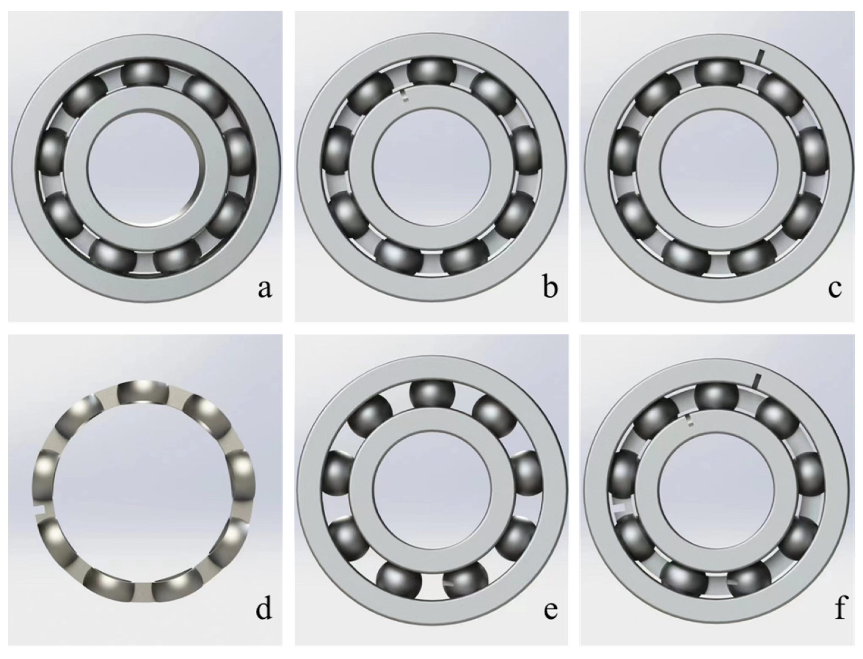
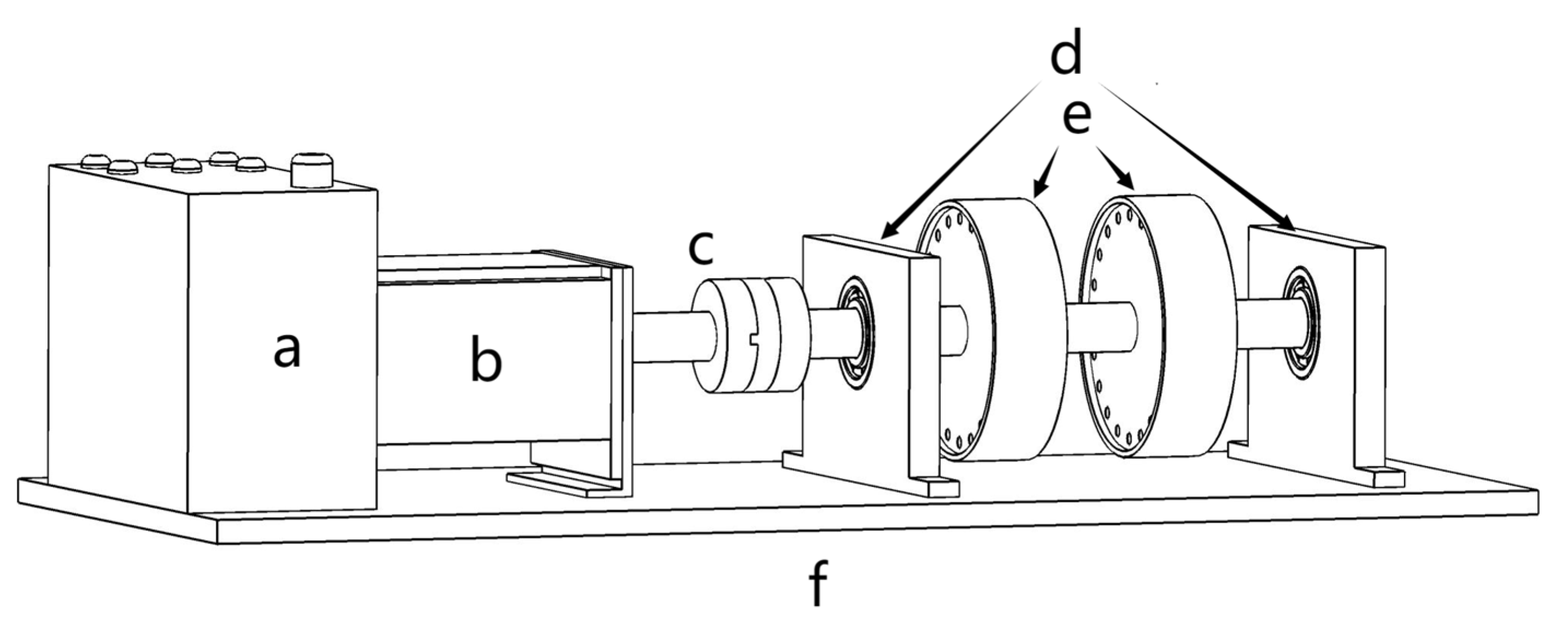
4.1. Dataset Description

In this study, bearing faults were meticulously fabricated using electrical discharge machining (EDM) technology to simulate various types of failures commonly encountered in industrial settings. Figure 2 illustrates the different conditions under which the bearings were examined. Figure 2a represents a healthy bearing, serving as the control specimen. Figure 2b depicts a bearing with an inner race defect, Figure 2c shows a bearing with an outer race defect, and Figure 2d presents a bearing with a cage defect. Figure 2e is indicative of a ball defect bearing, and Figure 2f illustrates a complex scenario of a mixed fault bearing, which incorporates defects in the inner race, outer race, cage, and balls, representing a comprehensive failure mode. The dimensions of the artificially induced defects were precisely controlled, with each fault characterized by a width of 0.3 mm and a depth of 0.15 mm.

The bearing test rig is shown in Figure 3. The core part of the rig’s control system is the controller (Part a in Figure 3), featuring an adjustment knob for fine-tuning the speed and the ability to reverse the direction of the motor to suit various testing scenarios. The controller is compatible with standard electrical systems, with a power specification of single-phase 220 V, 50 Hz. Powering the rig is a 100-W direct current (DC) brushless motor (Part b in Figure 3), reaching up to 3000 rpm, regulated by a DC controller to ensure steady speeds during operation.

Mechanical linkage within the rig is facilitated by membrane coupling (Part c in Figure 3), incorporating a membrane cushion for vibration damping. This coupling is designed to accommodate shafts ranging from 8 mm to 14 mm in diameter. The rig’s structure comprises front and rear bearing housings (Part d in Figure 3) constructed from premium aluminum alloy, featuring surfaces that are sandblasted and anodized for enhanced durability. The rotors (Part e in Figure 3), also constructed from similar materials and treated similarly, have dimensions of 80 mm in diameter and 20 mm in thickness. The rig’s base (Part f in Figure 3), made of aluminum alloy with anodic oxidation, measures 356 mm in length, 130 mm in width, and 14 mm in height, providing a robust platform for the entire setup. This meticulously engineered test rig, with its detailed specifications and adaptive control capabilities, serves as a critical instrument for bearing failure analysis, enabling extensive and controlled experimentation. The bore diameter measures 12 mm, the outside diameter is 28 mm, and the width of the bearing is quantified at 8 mm.

The physical photo of the experimental platform is shown in Figure 4. To capture bearing fault signals, a comprehensive set of equipment is utilized, including a single-axis accelerometer (model 333B30 was sourced from PCB Piezotronics, Inc., located in Depew, NY, USA) with a sensitivity of 10.11 mV/(m/s²) for precise vibration measurements. Data processing is facilitated by a robust PC, a notebook workstation from Dell (DELL Precision M3800, was manufactured by Dell Inc., located in Round Rock, TX, USA), chosen for its reliability and performance. The DAQ system, LMS SCADAS by Siemens (LMS SCADAS equipment is manufactured by Siemens Digital Industries Software, headquartered in Leuven, Belgium), ensures accurate data acquisition and signal analysis. Additionally, Siemens’s Testlab software (Version Testlab 2016) is employed for advanced analysis and interpretation of the captured signals. Bearing fault detection equipment is outlined in

Table 1. Bearing fault detection equipment.

Apparatus	Version	Producer	Sensitivity
Single-axis accelerometer	333B30	PCB	10.11 mV/(m/s2)
PC	Notebook workstation	Dell	-
DAQ system	LMS SCADAS	Siemens	-
Software	Testlab	Siemens	-

.

Figure 5 illustrates the experimental arrangement utilized for the detection of bearing faults, featuring the specific equipment outlined in Table 1. The experimental protocol necessitated the replacement of the bearing within the right-side bearing seat (Part a in Figure 5) with six uniquely conditioned bearings. This substitution protocol was vital for an exhaustive investigation into various bearing conditions, which included a standard bearing, and bearings with faults located in the inner race, outer race, cage, and balls, as well as a bearing manifesting combined faults.

The bearings were tested under a series of rotational speeds, namely, 1000, 1500, and 2000 rpm. Concurrently, vibration acceleration signals were rigorously recorded, with the placement and orientation of the PCB single-axis accelerometer, model 333B30, being situated as depicted in Part b in Figure 5. The data acquisition (DAQ) system employed was a Siemens LMS SCADAS (Part c in Figure 5), with a high-resolution sampling rate of 20,480 Hz. This sampling configuration was maintained throughout the experiment, with each bearing condition being sampled for a duration of five minutes. This comprehensive data collection methodology facilitated a detailed assessment of the vibrational attributes unique to each bearing fault category across the variable operational speeds.

For the data processing phase, Siemens’s Testlab software (Part d in Figure 5) was employed. This sophisticated analytical tool enabled the precise analysis and interpretation of the vibration data, contributing significantly to the study’s overall data analysis efficacy.

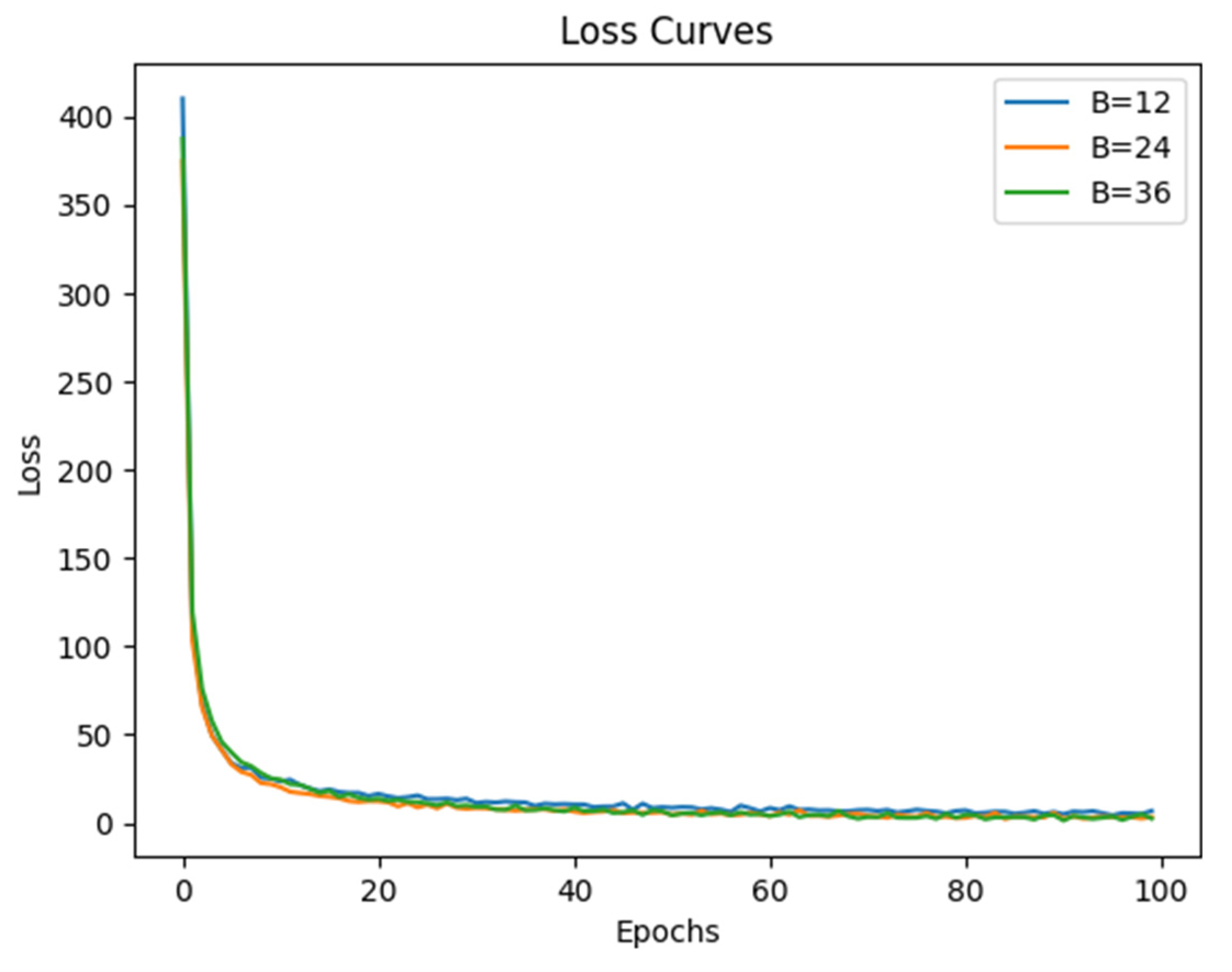
4.2. Parameter Setting

The rotation speeds of the data in the experiments are 1000, 1500 and 2000 rpm. One-hot labels are assigned corresponding to each sample. There are 197,328 samples in the training set, and there are 32,288 and 6450 samples in the test and validation sets, respectively.

The CQT spectral range is within 36 and 4608 Hz. The recordings are chopped into frames with 30 ms intervals. There are 90 frequency points per frame. There are six types of bearing faults, so the output dimension of the second GCN layer is set to 6. The first GCN layer produces a 450-dimensional output, and this output has the same dimensions as the input of the second GCN layer. Five consecutive frames of CQT spectra are concentrated together as the input feature, so M = 2. Cross-entropy is chosen as the loss function, and the Adam optimizer is employed for network optimization. The learning rate is set at 0.001, with training conducted for 1000 epochs.

All experiments were conducted on Windows 11(which is developed and maintained by Microsoft Corporation, headquartered in Redmond, Washington, DC, USA), utilizing an Intel i7 11800H CPU(Which is manufactured by Intel Corporation, headquartered in Santa Clara, CA, USA) running at 2.30 GHz and an NVIDIA RTX 3060 6 GB GPU (Which is manufactured by NVIDIA Corporation, headquartered in Santa Clara, CA, USA). The code, developed in the PyTorch framework, is written in Python 3.8.

4.3. Evaluation Metrics

We adopted five metrics, namely, accuracy, precision, F1 score, micro-average area under the ROC curve (AUC), and macro-average AUC, to comprehensively evaluate the model’s performance. Accuracy, the most intuitive performance metric, reflects the proportion of correctly classified samples by the model. It is defined as per [19]:

$$Accuracy=\frac{TP+TN}{TP+TN+FP+FN}$$

(11)

where TP represents the true positive instances, i.e., the number of samples correctly predicted as positive by the model. TN corresponds to the true negative instances, indicating the number of samples correctly predicted as negative. FP represents false-positive instances, denoting the number of samples incorrectly predicted as positive when they are actually negative. FN is associated with false-negative instances, representing the number of samples incorrectly predicted as negative when they are actually positive.

Precision emphasizes the accuracy of this model in predicting positive instances, measuring the proportion of true-positive instances among the samples predicted as positive by the model. It is defined as per [19]:

$$Precision=\frac{TP}{TP+FP}$$

(12)

Recall measures how many positive instances the model successfully captures among all actual positive samples. Specifically, it is the ratio of true positive instances to all actual positive instances, defined as per [19]:

$$Recall=\frac{TP}{TP+FN}$$

(13)

F1 score is a comprehensive performance metric that combines precision and recall, aiming to balance the trade-off between these two. It is the harmonic mean of these two metrics, and its calculation formula is as per [19]:

$$F1\text{-}score=\frac{2\cdot Precision\cdot Recall}{Precision+Recall}$$

(14)

Micro_AUC refers to micro-average AUC. Assume that TP_i represents the true-positive instances for the $i\text{-}\mathrm{th}$ category, FN_i represents the false-negative instances for the $i\text{-}\mathrm{th}$ category, and N is the total number of categories. Micro_AUC considers the overall performance across all bearing fault categories, providing a comprehensive measure of global performance. The formula is as per [24]:

$$Micro\_AUC=\frac{{\displaystyle \sum _{i=1}^{N}T}{P}_i}{{\displaystyle \sum _{i=1}^N(T{P}_i+F{N}_i)}}$$

(15)

Macro_AUC refers to macro-average AUC, which is a metric used to assess the performance of a model in multi-class classification tasks. In macro-average AUC, AUC is calculated for each class, and then these AUC values are averaged. Each class’s AUC is treated equally, without considering class imbalances. It is defined as per [24]:

$$Macro\_AUC=\frac{1}{N}{\displaystyle \sum _{i=1}^{N}A}U{C}_i$$

(16)

where N is the total number of categories, and $AU{C}_i$ represents the area under the curve (AUC) for the $i\text{-}\mathrm{th}$ category, defined as per [24]:

$$AU{C}_i\approx {\displaystyle \sum _{i=1}^n\frac{(TP{R}_i+TP{R}_{i-1})\cdot (FP{R}_i-FP{R}_{i-1})}{2}}$$

(17)

where $TP{R}_i$ represents the true-positive rate at the $i$-th threshold and $FP{R}_i$ represents the false-positive rate at the $i$-th threshold. The variable n corresponds to the number of selected thresholds. Assigning equal weights to the performance of the six fault categories helps alleviate the impact of class imbalance.

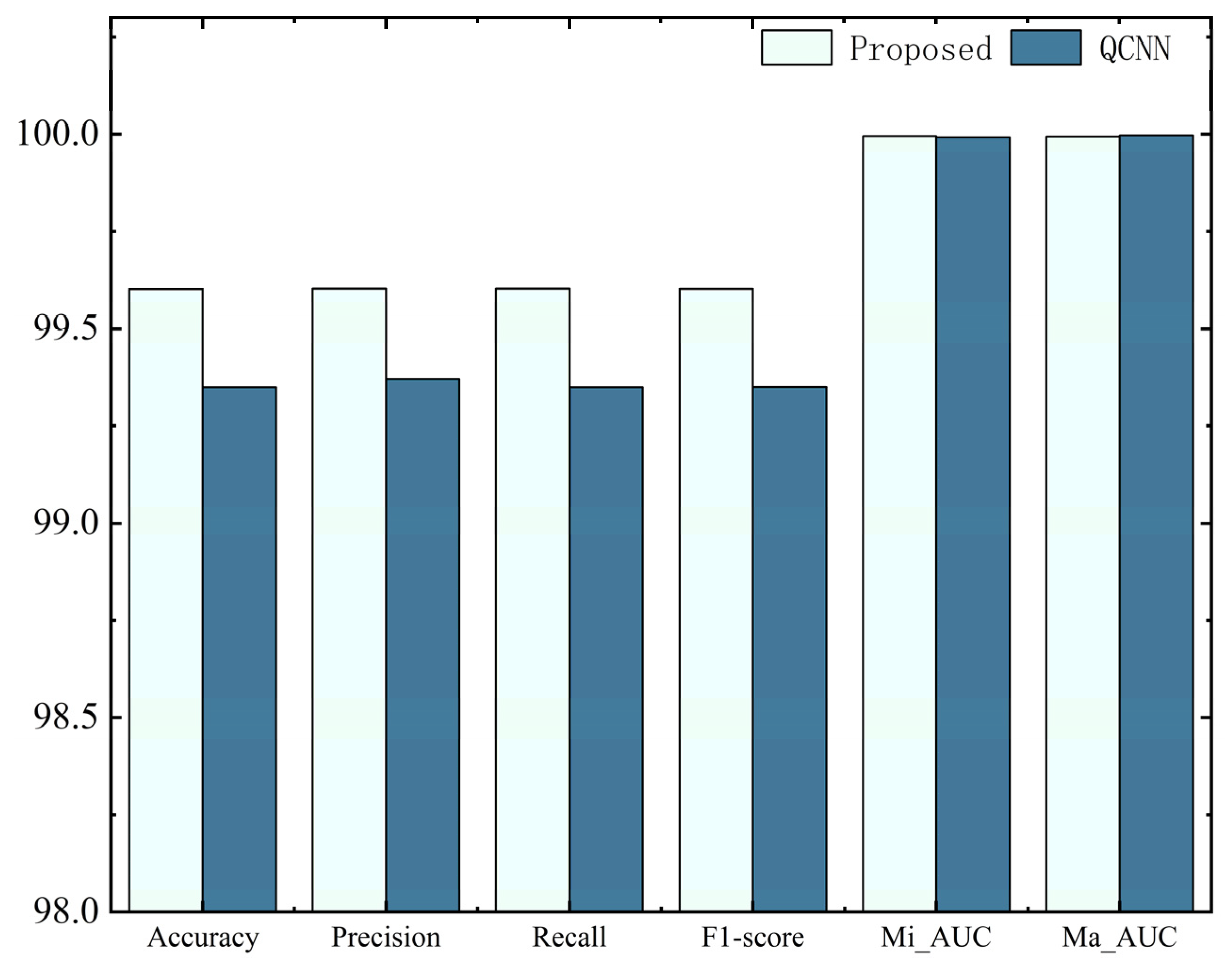
4.4. Experimental Results and Discussion

To investigate the impact of different CQT resolutions on the performance of our method, we selected three different values for B in the experiments, i.e., 12, 24, and 36. The loss curves are shown in Figure 6, where the horizontal axis represents the number of training iterations and the vertical axis represents the loss values. Preliminary observations indicate that the choice of B seems to have little influence on the overall change in loss.

To comprehensively assess the impact of B, we conducted further experiments. We evaluated the performance of the proposed model on validation set under three B values. As depicted in Figure 7, the model performs notably well when B is set to 12, outperforming the other two cases, though the differences are marginal. Therefore, B is set to 12 for lower computational costs while ensuring overall model performance.

The accuracy of the test set is shown in Figure 8. It can be seen from this figure that the proposed model performs slightly better than QCNN [17], and they both perform well on these five metrics. Furthermore, Mi_AUC and Ma_AUC accuracy is about 99.99%, indicating that the proposed model is robust to different fault types. Overall, our proposed bearing fault detection model demonstrates excellent performance in bearing fault diagnosis.

The confusion matrices are depicted in Figure 9. There are totally six types of bearing faults: “H” signifies normal bearing, “OR” denotes outer race fault, “IR” represents inner race fault, “MIX” corresponds to mixed fault, “B” indicates ball fault, and “C” represents cage fault. Each row in the figure represents the true labels, and each column signifies the predicted labels. The dark portions along the diagonal indicate the number of correctly predicted instances for each category. The numbers along the diagonal in the figure reveal that the majority of faults are accurately predicted. In addition, there are also some misclassifications. It can be seen from this figure that QCNN does not perform well for the cage fault since there are 177 samples misclassified as normal bearing, but it works well for the normal and ball faults. The proposed approach performs similar among different category samples, indicating the robustness of the proposed approach. However, the errors are still marginal, as illustrated in Figure 8 and Figure 9.

For intuitive observation of classification, we employed t-distributed stochastic neighbor embedding (t-SNE) to visualize the output features of the final convolutional layer, as presented in Figure 10. In this figure, different colors represent bearings of different fault categories. Upon observation, it is evident that the proposed model is effective in bearing fault diagnosis. It is noteworthy that in the figure, the points in green (denoting outer race fault bearings) are somewhat confused with purple points (denoting ball fault bearings). This indicates that a small proportion of outer race fault bearings are misidentified as ball fault bearings. In addition, the same type of fault with different rotation speeds is depicted in the same color. The points in red and purple are concentrated into three clusters, indicating that the fault features are also related with speed, so we focus on eliminating the influence of rotating speed in the future work. Compared with the proposed model, the t-SNE graph of QCNN is more complicated, indicating that features of QCNN are more diverse. Its intra-cluster distance is larger and inter-cluster distance is smaller than the proposed model.

5. Conclusions

This paper introduces a fault diagnosis approach for analyzing vibration signals using a GCN. The CQT spectrum of the vibration signal is first calculated. Subsequently, the CQT spectrum is transformed into a graph structure, where the frequency bins are modeled as nodes and their harmonic relationships are represented by edges. Finally, a two-layer GCN is employed to extract high-level features from the vibration signal and determine the fault type. The proposed approach effectively handles bearing fault diagnosis under different rotation speeds, showcasing robust generalization property. We have also compared its performance with one state-of-the-art bearing fault diagnosis model. Experimental results demonstrate that the proposed model achieves better performance across five evaluation metrics. According to t-SNE visualization, the proposed model is more effective in distinguishing features of different fault types.

References

1. Zhu, W.; Ni, G.; Cao, Y.; Wang, H. Research on a rolling bearing health monitoring algorithm oriented to industrial big data. Measurement 2021, 185, 110044. [Google Scholar] [CrossRef]
2. Liu, Y.; Chen, Z.; Wang, K.; Zhai, W. Surface wear evolution of traction motor bearings in vibration environment of a locomotive during operation. Sci. China Technol. Sci. 2022, 65, 920–931. [Google Scholar] [CrossRef]
3. Manieri, F.; Stadler, K.; Morales-Espejel, G.E.; Kadiric, A. The origins of white etching cracks and their significance to rolling bearing failures. Int. J. Fatigue 2019, 120, 107–133. [Google Scholar] [CrossRef]
4. Vasić, M.; Stojanović, B.; Blagojević, M. Failure analysis of idler roller bearings in belt conveyors. Eng. Fail. Anal. 2020, 117, 104898. [Google Scholar] [CrossRef]
5. Hasan, M.J.; Islam, M.M.; Kim, J.M. Acoustic spectral imaging and transfer learning for reliable bearing fault diagnosis under variable speed conditions. Measurement 2019, 138, 620–631. [Google Scholar] [CrossRef]
6. Gupta, P.; Pradhan, M.K. Fault detection analysis in rolling element bearing: A review. Mater. Today Proc. 2017, 4, 2085–2094. [Google Scholar] [CrossRef]
7. Zhang, Q.; Deng, L. An intelligent fault diagnosis method of rolling bearings based on short-time Fourier transform and convolutional neural network. J. Fail. Anal. Prev. 2023, 23, 795–811. [Google Scholar] [CrossRef]
8. Moshrefzadeh, A.; Fasana, A. The Autogram: An effective approach for selecting the optimal demodulation band in rolling element bearings diagnosis. Mech. Syst. Signal Process. 2018, 105, 294–318. [Google Scholar] [CrossRef]
9. Wu, K.; Chu, N.; Wu, D.; Antoni, J. The Enkurgram: A characteristic frequency extraction method for fluid machinery based on multi-band demodulation strategy. Mech. Syst. Signal Process. 2021, 155, 107564. [Google Scholar] [CrossRef]
10. Chen, X.; Guo, Y.; Na, J. Improvement on IESFOgram for demodulation band determination in the rolling element bearings diagnosis. Mech. Syst. Signal Process. 2022, 168, 108683. [Google Scholar] [CrossRef]
11. Hebda-Sobkowicz, J.; Zimroz, R.; Wyłomańska, A.; Antoni, J. Infogram performance analysis and its enhancement for bearings diagnostics in presence of non-Gaussian noise. Mech. Syst. Signal Process. 2022, 170, 108764. [Google Scholar] [CrossRef]
12. Alonso-González, M.; Díaz, V.G.; Pérez, B.L.; G-Bustelo, B.C.P.; Anzola, J.P. Bearing fault diagnosis with envelope analysis and machine learning approaches using CWRU dataset. IEEE Access 2023, 11, 57796–57805. [Google Scholar] [CrossRef]
13. Huzaifah, M. Comparison of time-frequency representations for environmental sound classification using convolutional neural networks. arXiv 2017, arXiv:1706.07156. [Google Scholar]
14. Zhang, S.; Zhang, S.; Wang, B.; Habetler, T.G. Deep learning algorithms for bearing fault diagnostics—A comprehensive review. IEEE Access 2020, 8, 29857–29881. [Google Scholar] [CrossRef]
15. Neupane, D.; Seok, J. Bearing fault detection and diagnosis using case western reserve university dataset with deep learning approaches: A review. IEEE Access 2020, 8, 93155–93178. [Google Scholar] [CrossRef]
16. Hoang, D.T.; Kang, H.J. A survey on deep learning based bearing fault diagnosis. Neurocomputing 2019, 335, 327–335. [Google Scholar] [CrossRef]
17. Liao, J.X.; Dong, H.C.; Sun, Z.Q.; Sun, J.; Zhang, S.; Fan, F. Attention-embedded quadratic network (qttention) for effective and interpretable bear-ing fault diagnosis. IEEE Trans. Instrum. Meassurement 2023, 72, 1–13. [Google Scholar] [CrossRef]
18. Qi-Yu, T.A.N.; Ping, M.A.; Hong-Li, Z.H.A.N.G. Fault Diagnosis of Rolling Bearings Based on Graph Convolutional Networks. Noise Vib. Control 2023, 43, 101. [Google Scholar]
19. Zhang, F.; Jin, Q.; Li, D.; Zhang, Y.; Zhu, Q. Physical Graph-Based Spatiotemporal Fusion Approach for Process Fault Diagnosis. ACS Omega 2024, 9, 9486–9502. [Google Scholar] [CrossRef]
20. Yang, G.; Yao, J. Multilayer neurocontrol of high-order uncertain nonlinear systems with active disturbance rejection. Int. J. Robust Nonlinear Control 2024, 34, 2972–2987. [Google Scholar] [CrossRef]
21. Yang, G. Asymptotic tracking with novel integral robust schemes for mismatched uncertain nonlinear systems. Int. J. Robust Nonlinear Control 2023, 33, 1988–2002. [Google Scholar] [CrossRef]
22. Schörkhuber, C.; Klapuri, A. Constant-Q transform toolbox for music processing. In Proceedings of the 7th Sound and Music Computing Conference, Barcelona, Spain, 21–24 July 2010; pp. 3–64. [Google Scholar]
23. Zhang, W.; Yan, L.; Zhang, Q.; Gao, J. Graph modeling for vocal melody extraction from polyphonic music. Appl. Acoust. 2023, 211, 109491. [Google Scholar] [CrossRef]
24. Yang, Y. An evaluation of statistical approaches to text categorization. Inf. Retr. 1999, 1, 69–90. [Google Scholar] [CrossRef]
Figure 1. Proposed approach. Different colors are utilized to represent different layers.
Machines 12 00179 g001
Figure 2. Bearing fault types. (a) A healthy bearing. (b) Bearing with inner race defect. (c) Bearing with outer race defect. (d) Bearing with cage defect. (e) Bearing with ball defect. (f) Bearing with mixed faults.
Machines 12 00179 g002
Figure 3. Bearing test rig.
Machines 12 00179 g003
Figure 4. Experimental platform.
Machines 12 00179 g004
Figure 5. Bearing fault detection equipment.
Machines 12 00179 g005
Figure 6. Loss curves of the training set.
Machines 12 00179 g006
Figure 7. The evaluation results with respect to different metrics on validation set.
Machines 12 00179 g007
Figure 8. Evaluation results with respect to different metrics on test set.
Machines 12 00179 g008
Figure 9. Confusion matrices.
Machines 12 00179 g009
Figure 10. t-SNE results of features produced by the last convolutional layer.
Machines 12 00179 g010