Tool Wear Monitoring System Using Seq2Seq

Abstract

The advancement of smart factories has brought about small quantity batch production. In multi-variety production, both materials and processing methods change constantly, resulting in irregular changes in the progression of tool wear, which is often affected by processing methods. This leads to changes in the timing of tool replacement, and failure to correctly determine this timing may result in substantial damage and financial loss. In this study, we sought to address the issue of incorrect timing for tool replacement by using a Seq2Seq model to predict tool wear. We also trained LSTM and GRU models to compare performance by using ${\mathrm{R}}^2$, mean absolute error (MAE), and mean squared error (MSE). The Seq2Seq model outperformed LSTM and GRU with an ${\mathrm{R}}^2$ of approximately 0.03~0.037 in step drill data, 0.540.57 in top metal data, and 0.16~0.45 in low metal data. Confirming that Seq2Seq exhibited the best performance, we established a real-time monitoring system to verify the prediction results obtained using the Seq2Seq model. It is anticipated that this monitoring system will help prevent accidents in advance.

1. Introduction

In the past, customers’ needs were satisfied mainly with products supplied to the market by manufacturers or distributors. However, with technological advancements, most industrial fields have undergone segmentation, diversification, and specialization, which have contributed to fostering an atmosphere that respects individual diversity [1]. As a result, consumer demands have become more diverse, requiring specific forms and types of consumption to meet each person’s unique preferences. This has highlighted the importance of customized production, giving rise to the demand for multi-variety production [2]. Furthermore, in factories, as there are tasks requiring skilled expertise, many people are involved in the manufacturing process. However, the decreasing workforce due to social issues such as low birth rates and aging populations around the world is leading to a reduction in the number of people able to work in factories [3].

For these reasons, smart factories are gaining attention in the manufacturing sector. Smart factories not only enable mass production of multiple products but they are also equipped with sensors to collect and analyze data on equipment and machines within the factory, and to allow for autonomous control according to a given purpose. This offers the advantage of allowing less skilled workers to address issues even in situations where the subjective judgment of experienced workers is required. As factory equipment continues to operate, damage may occur due to wear and tear, cracks, etc. This can lead to catastrophic accidents or operational shutdowns, resulting in significant damage and financial losses [4]. Therefore, tools should be replaced in a timely manner according to their predetermined lifecycle. However, as their lifecycle varies depending on the processing method, there is a risk of incorrectly determining the lifecycle during multi-variety production. This issue adversely affects the productivity and economic efficiency of the factory. To address this challenge, research is currently underway to predict tool wear by utilizing data acquired through sensors, which could help prevent accidents by forecasting the lifespan of tools.

Jang et al. [3] obtained vibration data by using an accelerometer and compared the data before and after tool wear by applying Fast Fourier Transform (FFT) and a Butterworth filter to the data. They then trained a convolutional neural network (CNN) using both the Butterworth filter preprocessed data and raw data. The results showed that the CNN model trained with raw data achieved performance exceeding 95% accuracy, outperforming the model trained with the Butterworth filter preprocessed data. Lee et al. [5] classified the tool wear condition using the Xgboost, random forest (RF), and support vector machine (SVM) by utilizing data such as power, current, feed rate, and coordinate values of the X, Y, and Z axes and the spindle used in CNC machines. RF was found to demonstrate the most outstanding performance considering both time consumption and accuracy. Choi et al. [6] utilized vibration data obtained from vibration sensors in core multi-processing, and acceleration and current data collected from accelerometers to calculate the maximum, average, and standard deviation per unit time. Prediction was then performed using four different kernels for support vector regression (SVR). The resulting prediction performance was compared by using root mean square error (RMSE), mean absolute error (MAE), and mean absolute percentage error (MAPE). It was found that the best performance was achieved when the Gaussian kernel was used. Oh et al. [7] measured cutting forces using voltage and predicted tool wear by training an autoassociative neural network (AANN) with the average, effective value, and feed rate, which are sensitive to wear types and degrees. Because these studies train models with feature points extracted from obtained data to predict the current state or degree of tool wear, they may encounter difficulty in responding to sudden changes, such as changes in processing methods.

In this paper, we aimed to predict future, rather than current, tool wear using Seq2Seq, a model that takes sequence data as input and produces sequence data as output, without extracting feature points from the data obtained from a factory. To evaluate the performance after prediction, we compared it with existing recurrent neural network models using ${\mathrm{R}}^2$, MAE, and mean squared error (MSE). In addition, we developed a monitoring system to check the prediction results on a real-time basis.

The content of this paper is as follows: Section 2 explores existing studies on tool wear prediction. Section 3 explains the models used to predict tool wear. Section 4 describes the experimental setup and results, and Section 5 provides conclusions of this study.

2. Related Works

Research on tool wear prediction has been vigorously carried out at home and abroad, with many studies applying deep learning and machine learning methods. Tools used in machining equipment such as drills, milling machines, and CNC machines require replacement according to a specified replacement cycle. Failure to replace tools in a timely manner according to this cycle can lead to wear and errors during the product manufacturing process, resulting in a deterioration of product quality. Therefore, the replacement of worn tools is essential to ensure product quality. The key aspect of tool replacement lies in not exceeding a certain level of wear. Typically, on-site tool replacement follows a fixed cycle recommended by machine/tool manufacturers. However, using a fixed cycle for tool replacement poses challenges as it may not align with the wear cycles based on combinations of products, raw materials, and processing methods. Hence, the universally recommended replacement cycle from manufacturers is less likely to correspond to conditions in actual manufacturing settings. In other words, replacing tools too early can lead to increased replacement costs, while delayed replacements may result in an increase in defective products. To address this challenge, data analysis techniques involve a model that defines the factor variable by measuring the wear state of tools with sensors such as resistance, vibration, current, acoustic emission, and temperature while also defining the degree of tool wear as the target variable. This model for predicting tool wear is constructed by using methods such as an artificial neural network (ANN) and support vector machine (SVM) [8,9].

Most methodologies for analyzing unstructured manufacturing data are fundamentally rooted in information and communication technology (ICT). In ICT, sensors are often utilized to acquire sensor data, and algorithms and prediction models suitable for this data are developed. For the prediction and analysis of manufacturing data, most basic models such as SVM, ANN, RF, DT, etc., are commonly used to build well-generalized models [10].

Researchers overseas have extensively investigated the prediction of machining errors caused by the tool surface and frictional forces during the machining process. Aghazadeh et al. [11] utilized vibration, signal, and press data of sensors along with a convolutional neural network (CNN) model to develop a tool conditioning monitoring (TCM) system. Kong et al. [12] addressed tool wear and cutting load issues by predicting the extent of wear using radial basis functions (RBF), principal component analysis (PCA), and Gaussian process regression (GPR) models. Furthermore, to apply these findings industrially, they employed autoregressive (AR) models, moving average (MA) models, or autoregressive moving average (ARMA) hybrid models. Zhou et al. [13] also utilized multiple sensors to acquire data, and then tracked the efficient tool state using artificial intelligence (AI) models and efficiently predicted replacement timing [14,15].

Hassan et al. [16] analyzed correlations between the machined surface and the tool in the turning process to correct the detachment degree, and they predicted tool errors and wear degrees. Rech et al. [17] used contact pressure and sliding speed to calculate friction conditions related to the degree of tool wear for each tool during turning, and performed post-prediction using the calculated settings. Scheffer et al. [18] employed an AI model to monitor tool wear during hard turning. They used data such as cutting forces, vibrations, and temperature, and utilized a self-organizing map (SOM) model for training. Ozel et al. [19] used a neural network model to predict tool wear and surface roughness. This model enabled an improvement in the tool wear trend and machining efficiency.

3. Tool Wear Prediction Model

The system structure for predicting the wear of the rotary index machine in this paper is shown in Figure 1. As shown in Figure 1, EOCR is installed at the rotary index to acquire step drill, upper metal, and lower metal data, respectively. These data refer to the tool for machining the rotary index. First, there is the preprocessing of the acquired data, and second, a methodology for accurately predicting current data, which are important for predicting wear, is introduced using an AI model. And finally, it shows the results of testing by applying it to an actual system.

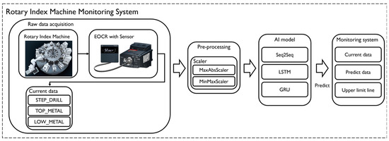
Figure 1. System overview.

3.1. Data Composition and Preprocessing

Current data were obtained from the tool using EOCR and sensors on a rotary indexing machine from Hyeopseong Tech, Changwon, Korea. In this study, current data from step drills, top metal, and low metal were used. For each tool, three types of current data were collected and experiments were conducted by applying each datum to the model for training.

Data for step drills and top metals were collected every 100 ms over a period of one month, resulting in approximately 25 million pieces of data. Null or zero values in the data are removed through preprocessing because they indicate that the machine is not working. To be able to use it for model learning, a sliding window method is applied, as shown in Figure 2. This method uses 100 pieces of current state data and preprocesses them to predict the 100 next state data. A total of 2526 pieces of data were created in this way, of which 80% were used for learning and 10% for testing.

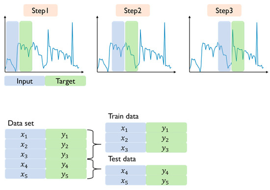
Figure 2. Data to convert.

To prepare the data created through the above process for training, various scalers from sklearn, including StandardScaler, MinMaxScaler, MaxAbsScaler, RobustScaler, and Normalizer, were applied to each dataset. After experimenting with different scalers, it was found that MinMaxScaler yielded the best results for step drills, whereas MaxAbsScaler was the most effective for top metal and low metal. Therefore, MinMaxScaler and MaxAbsScaler were used for scaling before training. Figure 3 shows the data before and after scaling.

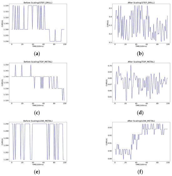
Figure 3. Comparison of data distribution with and without scaling: (a) STEP_DRILL raw data; (b) STEP_DRILL after using MaxAbsScaler; (c) TOP_METAL raw data; (d) TOP_METAL after using MinMaxScaler; (e) LOW_METAL raw data; (f) LOW_METAL after using MinMaxScaler.

3.2. Long Short-Term Memory (LSTM)

LSTM passes the Hidden State and Cell State to the next cell, and the Hidden State and Cell State are then updated through forget, input, and output gates. Figure 4 illustrates the LSTM architecture. The current input ${\mathrm{x}}_{\mathrm{t}}$ passes through a sigmoid function, resulting in values ${\mathrm{f}}_{\mathrm{t}}$, ${\mathrm{i}}_{\mathrm{t}}$, and ${\mathrm{o}}_{\mathrm{t}}$ between 0 and 1, which are then used for the forget, input, and output gates, respectively. The forget gate, referencing ${\mathrm{x}}_{\mathrm{t}}$ and the previous state ${\mathrm{h}}_{\mathrm{t}-1}$, determines how much information to forget. If ${\mathrm{f}}_{\mathrm{t}}$ is 0, everything is forgotten, and if it is 1, no information is forgotten, determining the amount of information the Cell State will take. The input gate, determining how much information to utilize, applies ${\mathrm{i}}_{\mathrm{t}}$ and ${\mathrm{x}}_{\mathrm{t}}$ to the tangent function, adding the resulting $\widetilde{{\mathrm{C}}_{\mathrm{t}}}$ to the Cell State. After passing through the forget gate and input gate, the Cell State is completed as ${\mathrm{C}}_{\mathrm{t}}$, which is then passed to the next cell. The output gate multiplies the value to which the tangent function was applied by the completed Cell State, with ${\mathrm{o}}_{\mathrm{t}}$, resulting in the Hidden State ${\mathrm{h}}_{\mathrm{t}}$ that is passed to the next cell. This process repeats for subsequent cells.

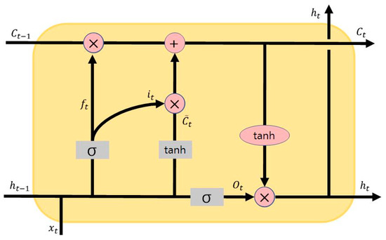
Figure 4. LSTM architecture.

3.3. Gated Recurrent Unit (GRU)

Figure 5 depicts the GRU architecture. Unlike LSTM, GRU does not have a Cell State, but the Hidden State plays the role of both the Hidden State and the Cell State. Whereas LSTM has three gates, GRU has two gates: the reset gate and the update gate. The reset gate determines how much of the past information to forget. It applies a sigmoid function to the input value ${\mathrm{x}}_{\mathrm{t}}$ and the previous state ${\mathrm{h}}_{\mathrm{t}-1}$, resulting in ${\mathrm{r}}_{\mathrm{t}}$, which is then multiplied by ${\mathrm{x}}_{\mathrm{t}}$ and ${\mathrm{h}}_{\mathrm{t}-1}$, resetting the information based on the values between 0 and 1. The update gate decides which information, between the past and present, to update further. It forgets 1 − ${\mathrm{z}}_{\mathrm{t}}$ amount of information from the Hidden State, then applies the tangent function to ${\mathrm{x}}_{\mathrm{t}}$, which has just passed the reset gate, multiplying the resulting value $\widetilde{{\mathrm{h}}_{\mathrm{t}}}$ by ${\mathrm{r}}_{\mathrm{t}}$ and adding it to the Hidden State before passing it to the next cell. This process plays the same role as LSTM’s input and forget gates combined. Therefore, GRU has the advantage of faster processing speed due to fewer gates compared to LSTM.

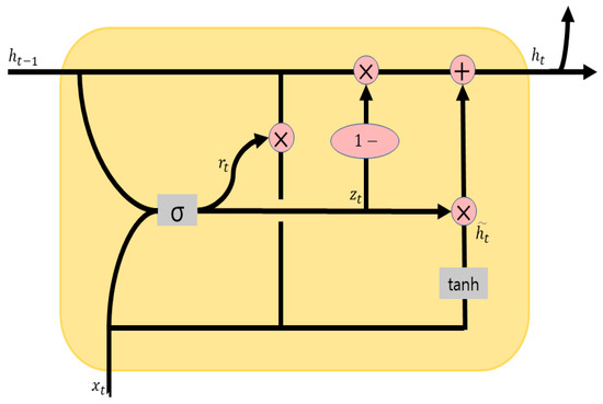
Figure 5. GRU architecture.

3.4. Sequence-to-Sequence (Seq2Seq)

Seq2Seq plays a role in converting sequence data from one domain to sequence data in another domain. Figure 6 illustrates the overall architecture of Seq2Seq. As shown in Figure 6, it consists of an encoder and a decoder, both consisting of models based on recurrent neural networks. The encoder compresses input sequence data in a Many-to-One fashion, creating a fixed-size vector called the context vector, which refers to the Hidden State of the encoder’s final state. The decoder operates in a Many-to-Many fashion, receiving this context vector as the initial state and predicting sequence data. The role of the encoder can be expressed by Equations (1) and (2). Here, m is the size of the input time step, ${\mathrm{x}}_{\mathrm{t}}$ is the input, and ${{\mathrm{h}}_{\mathrm{t}}}^{\mathrm{enc}}$ represents the state at time step t, where t is an integer from 1 to m. The encoder, like a traditional recurrent neural network, iteratively updates the current state ${{\mathrm{h}}_{\mathrm{t}}}^{\mathrm{enc}}$ using ${\mathrm{x}}_{\mathrm{t}}$ and the previous state ${{\mathrm{h}}_{\mathrm{t}-1}}^{\mathrm{enc}}$. After repeating this process, the concatenated ${{\mathrm{h}}_{1:\mathrm{m}}}^{\mathrm{enc}}$ becomes the context vector.

$${{\mathrm{h}}_{\mathrm{t}}}^{\mathrm{enc}}={\mathrm{RNN}}_{\mathrm{enc}}\left({\mathrm{x}}_{\mathrm{t}},{{\mathrm{h}}_{\mathrm{t}-1}}^{\mathrm{enc}}\right),\mathrm{where} {{\mathrm{h}}_0}^{\mathrm{enc}}$$

(1)

$${{\mathrm{h}}_{1:\mathrm{m}}}^{\mathrm{enc}}=\left[{{\mathrm{h}}_1}^{\mathrm{enc}};{{\mathrm{h}}_2}^{\mathrm{enc}};\dots ;{{\mathrm{h}}_{\mathrm{m}}}^{\mathrm{enc}}\right]$$

(2)

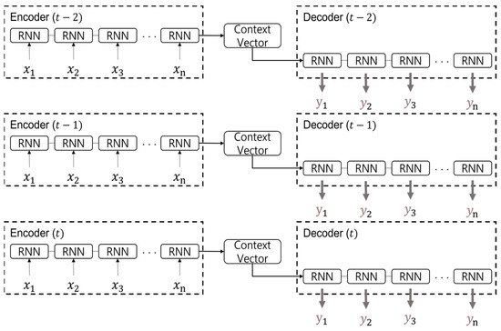
Figure 6. Seq2Seq architecture.

The role of the decoder can be expressed by Equations (3) and (4). Here, n is the size of the output time step, ${{\mathrm{h}}_{\mathrm{t}}}^{\mathrm{dec}}$ represents the state at time step t, where t is an integer from 1 to n, and ${{\mathrm{h}}_{\mathrm{m}}}^{\mathrm{enc}}$ is the context vector. In the first time step, as ${{\mathrm{h}}_{\mathrm{t}-1}}^{\mathrm{dec}}$ is ${{\mathrm{h}}_0}^{\mathrm{dec}}$, ${{\mathrm{h}}_{\mathrm{m}}}^{\mathrm{enc}}$ is used as the initial state. Then, in the subsequent RNN cell, ${{\mathrm{h}}_{\mathrm{m}}}^{\mathrm{enc}}$ and ${{\mathrm{h}}_{\mathrm{t}-1}}^{\mathrm{dec}}$ are used to calculate the output and the next ${{\mathrm{h}}_{\mathrm{t}}}^{\mathrm{dec}}$ to be passed to the next time step. When the length of the time step is n, the completed ${{\mathrm{h}}_1}^{\mathrm{dec}}$ to ${{\mathrm{h}}_{\mathrm{t}}}^{\mathrm{dec}}$ obtained through the above process is connected, and the concatenated ${{\mathrm{h}}_{1:\mathrm{n}}}^{\mathrm{dec}}$ is the final output.

$${{\mathrm{h}}_{\mathrm{t}}}^{\mathrm{dec}} = {\mathrm{RNN}}_{\mathrm{dec}}\left({{\mathrm{h}}_{\mathrm{m}}}^{\mathrm{enc}},{{\mathrm{h}}_{\mathrm{t}-1}}^{\mathrm{dec}}\right),\mathrm{where} {{\mathrm{h}}_0}^{\mathrm{dec}}={{\mathrm{h}}_{\mathrm{m}}}^{\mathrm{enc}}$$

(3)

$${{\mathrm{h}}_{1:\mathrm{n}}}^{\mathrm{dec}} = \left[{{\mathrm{h}}_1}^{\mathrm{dec}};\dots ;{{\mathrm{h}}_{\mathrm{n}}}^{\mathrm{dec}}\right]$$

(4)

3.5. Visualization and Prediction System

In this paper, a real-time monitoring system was established to verify the data predicted by using existing data. In Figure 7, from left to right, the data for step drills, top metal, and low metal are plotted. The top part represents the current values, while the bottom part represents the predicted values. The numerical values are indicated by blue lines, and the threshold is represented by a red line.

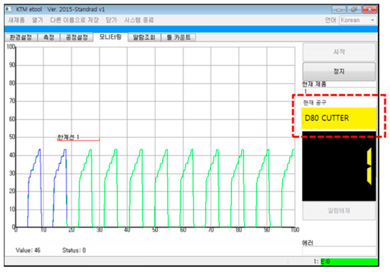
Figure 7. Real-time monitoring system overview.

4. Experimental Setup and Results

4.1. Experimental Setup

For the experiment in this study, Linux 18.04 was used as the operating system and Xeon Silver 4214 CPU was used, along with 256 GB of memory and RTX 3090 as the GPU. The deep learning framework used was Tensorflow 2.4.0.

We considered three models to find the optimal model to be used in the rotary index. First, the models used for training were Seq2Seq, LSTM, and GRU. The hyperparameters used in the model were set as follows. SGD was used as the optimization function and the initial learning rate was 0.01. Then, polynomial scheduling was used to transform the learning rate from 0.01 to 0.0001, and training was performed with RELU as the activation function and MSE as the loss function. And the cell size used in Seq2Seq, LSTM, and GRU was fixed to 64. There was a problem with decreased accuracy when the cell size was adjusted to be larger or smaller.

4.2. Experimental Results

The performance evaluation metrics ${\mathrm{R}}^2$, MAE, and MSE were used for comparison, where ${\mathrm{R}}^2$ is better when closer to 1, while MAE and MSE are better when closer to 0. The recurrent neural network model used as the encoder–decoder for Seq2Seq consisted of LSTM and GRU. When training only on the step drill data and comparing the performance using the ${\mathrm{R}}^2$ metric, the LSTM-based model achieved a score of 0.874913, while the GRU-based model scored 0.876063, showing similar performance. Therefore, only the Seq2Seq model composed of LSTM was used in this study.

Table 1 shows the results of each model for the step drill tool data. In Table 1, Seq2Seq exhibits a performance improvement of approximately 0.03~0.037 in ${\mathrm{R}}^2$ compared to LSTM and GRU. Meanwhile, MAE shows a difference of approximately 0.0028~0.0035, and MSE shows a difference of around 0.00033~0.00041. Table 2 presents the results for the top metal tool data. In Table 2, Seq2Seq demonstrates a performance improvement of about 0.54~0.57 in ${\mathrm{R}}^2$ compared to LSTM and GRU. Meanwhile, MAE shows a difference of approximately 0.018~0.019, and MSE shows a difference of around 0.001508~0.00152. Table 3 displays the results for the low metal tool data. In Table 3, Seq2Seq exhibits a performance improvement of approximately 0.16~0.45 in ${\mathrm{R}}^2$ compared to LSTM and GRU. Meanwhile, MAE shows a difference of approximately 0.0034~0.0014, and MSE shows a difference of around 0.00009~0.00013.

Table 1. Comparison of STEP_DRILL data results by model (cell size 64).

	${\mathbf{R}}^2$	MAE	MSE
Seq2Seq	0.874913	0.0231	0.001275
LSTM	0.837303	0.026649	0.001681
GRU	0.844892	0.025988	0.001602

Table 2. Comparison of TOP_METAL data results by model (cell size 64).

	${\mathbf{R}}^2$	MAE	MSE
Seq2Seq	0.894669	0.010283	0.000297
LSTM	0.353403	0.028393	0.001817
GRU	0.32174	0.02907	0.001805

Table 3. LOW_METAL results by model (cell size 64).

	${\mathbf{R}}^2$	MAE	MSE
Seq2Seq	0.764504	0.005457	0.000007
LSTM	0.314495	0.008868	0.00014
GRU	0.605802	0.006888	0.000101

Therefore, it can be said that the Seq2Seq model, with ${\mathrm{R}}^2$ being the closest to 1 and MAE/MSE approaching 0 in all tool data, demonstrated the most outstanding performance.

Figure 8 shows the experimental results in graphs, where the blue solid line represents the actual values, and the red dotted line represents the predicted values. The closer the red line is to the blue line, or even matches it, the better the prediction is. Figure 8 shows three graphs for each dataset for easy comparison of the experimental results, with the blue line representing the actual values, the red dotted line denoting the predicted values of the GRU model, the purple dotted line representing the predicted values of the LSTM model, and the green dotted line denoting the predicted values of the Seq2Seq model.

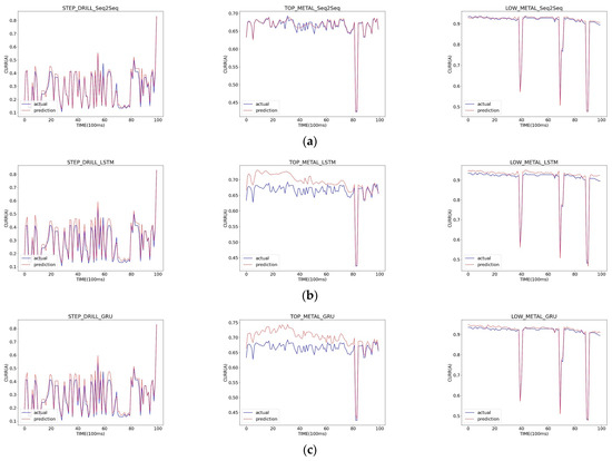
Figure 8. STEP_DRILL (left), TOP_METAL (center), and LOW_METAL (Right) prediction results by model: (a) Seq2Seq; (b) LSTM; (c) GRU.

When looking at graphs in Figure 8 and Figure 9 together, it can be observed that the step drill data are predicted similarly in all models and that for the top metal data, Seq2Seq outperforms LSTM and GRU in terms of prediction. However, for the low metal data, although there is a significant difference in ${\mathrm{R}}^2$, MAE and MSE show only marginal differences compared to the other datasets, making the difference less noticeable in the graphs. As a result of analyzing the results of these experiments, we were able to confirm that Seq2Seq was the model to be used in the field with the best performance.

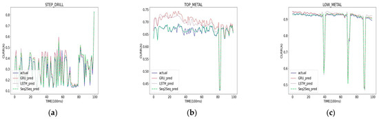
Figure 9. Comparison of prediction results by model: (a) STEP_DRILL; (b) TOP_METAL; (c) LOW_METAL.

Through previous experiments, we have confirmed that Seq2Seq has the best performance. Therefore, we performed further experiments by resizing the context vector. As a result of the experiments, while adjusting the size of the context vector, it was confirmed that the highest performance was achieved when the size was set to 64 (Table 4). Therefore, we are going to use Seq2Seq with a cell size of 64 for our system.

Table 4. Comparison of Seq2Seq measurements by cell size.

Vector Size	${\mathbf{R}}^2$	MAE	MSE
32	0.759504	0.005057	0.000005
64	0.764504	0.005457	0.000007
128	0.705802	0.006088	0.000011

5. Conclusions

In this paper, we addressed the failure to replace tools at the correct time due to multi-variety production in factories and the decreased problem-solving capability due to the reduction in skilled workers. To tackle these problems, we developed a monitoring system that can predict tool wear using the Seq2Seq model, which consists of an encoder and decoder based on a recurrent neural network.

We created data using the sliding window method to predict wear, trained the model, tested it, and evaluated its performance using R², MAE, and MSE metrics. As a result, the Seq2Seq model was found to improve R² from approximately 0.03 to 0.037 for step drill, from approximately 0.54 to 0.57 for top metal, and from approximately 0.16 to 0.45 for low metal. Additionally, as a result of testing while adjusting the size of the context vector, it was confirmed that the best performance was achieved with a cell size of 64.

Our future research is focused on improving the preprocessing methodology or model to improve its wear prediction accuracy. In addition, we plan to develop a model by adding EOCR and sensors to conduct an overall analysis to determine under what circumstances the tool wear of the rotary index machine is affected.

References

- Various Forms of Recent Consumption and Its Meaning. 2021. Available online: http://gspress.cauon.net/news/articleView.html?idxno=22284 (accessed on 30 January 2023).
- Kim, J.H.; Kim, D.C.; Je, S.H.; Lee, J.S.; Kim, D.H.; Ji, S.H. A Study on the Establishment of Prediction Conservation System for Smart Factory Facilities. In Proceedings of the Fall Conference of Korea Institute of Information Technology, Gyeongju, Republic of Korea, 16–18 November 2022; pp. 703–706. [Google Scholar]
- Jhang, S.S.; Song, Y.H.; Kwon, J.Y.; Lee, H.J.; Song, M.C.; Lee, J.S. Research on CNN-based learning, cutting tool condition analysis. In Proceedings of the Fall Conference of Korean Institute of Information Technology, Gyeongju, Republic of Korea, 16–18 November 2022; pp. 55–58. [Google Scholar]
- Lee, Y.H.; Kim, K.J.; Lee, S.I.; Kim, D.J. Seq2Seq model-based Prognostics and Health Management of Robot Arm. J. Korea Inst. Inf. Electron. Commun. Technol. 2019, 12, 242–250. [Google Scholar]
- Lee, K.B.; Park, S.H.; Sung, S.H.; Park, D.M. A Study on the Prediction of CNC Tool Wear Using Machine Learning Technique. J. Korea Converg. Soc. 2019, 10, 15–21. [Google Scholar]
- Choi, S.J.; Lee, S.J.; Hwang, S.G. Machine Learning Data Analysis for Tool Wear Prediction in Core Multi Process Machining. J. Korean Soc. Manuf. Process Eng. 2021, 20, 90–96. [Google Scholar] [CrossRef]
- Oh, D.J.; Sim, B.S.; Lee, W.K. Tool Wear Monitoring during Milling Using an Autoassociative Neural Network. J. Korean Soc. Mech. Eng. 2021, 45, 285–291. [Google Scholar] [CrossRef]
- Li, B. A Review of Tool Wear Estimation Using Theoretical Analysis and Numerical Simulation Technologies. Int. J. Refract. Met. Hard Mater. 2012, 35, 143–151. [Google Scholar] [CrossRef]
- Siddhpura, A.; Paurobally, R. A Review of Flank Wear Prediction Methods for Tool Condition Monitoring in a Turning Process. Int. J. Adv. Manuf. Technol. 2013, 65, 371–393. [Google Scholar] [CrossRef]
- Murphy, K.P. Machine Learning: A Probabilistic Perspective; The MIT Press: Cambridge, MA, USA, 2012. [Google Scholar]
- Aghazadeh, F.; Tahan, A.; Thomas, M. Tool Condition Monitoring Using Spectral Subtraction Algorithm and Artificial Intelligence Methods in Milling Process. Int. J. Mech. Eng. Robot. Res. 2018, 7, 30–34. [Google Scholar] [CrossRef]
- Kong, D.; Chen, Y.; Li, N. Gaussian process regression for tool wear prediction. Mech. Syst. Signal Process. 2018, 104, 556–574. [Google Scholar] [CrossRef]
- Zhou, Y.; Xue, W. Review of tool condition monitoring methods in milling processes. Int. J. Adv. Manuf. Technol. 2018, 96, 2509–2523. [Google Scholar] [CrossRef]
- Khorasani, A.; Yazdi, M.R.S. Development of a dynamic surface roughness monitoring system based on artificial neural networks (ANN) in milling operation. Int. J. Adv. Manuf. Technol. 2017, 93, 141–151. [Google Scholar] [CrossRef]
- Kong, D.; Chen, Y.; Li, N. Hidden semi-Markov model-based method for tool wear estimation in milling process. Int. J. Adv. Manuf. Technol. 2017, 92, 3647–3657. [Google Scholar] [CrossRef]
- Hassan, M.; Sadek, A.; Damir, A.; Attia, M.H.; Thomson, V. A novel approach for real-time prediction and prevention of tool chipping in intermittent turning machining. Manuf. Technol. 2018, 67, 41–44. [Google Scholar] [CrossRef]
- Rech, J.; Giovenco, A.; Courbon, C.; Cabanettes, F. Toward a new tribological approach to predict cutting tool wear. CIRP Ann. Manuf. Technol. 2018, 67, 65–68. [Google Scholar] [CrossRef]
- Scheer, C.; Kratz, H.; Heyns, P.S.; Klocke, F. Development of a tool wear-monitoring system for hard turning. Int. J. Mach. Tools Manuf. 2003, 43, 973–985. [Google Scholar]
- Ozel, T.; Karpat, Y. Predictive modeling of surface roughness and tool wear in hard turning using regression and neural networks. Int. J. Mach. Tools Manuf. 2005, 45, 467–479. [Google Scholar] [CrossRef]
Disclaimer/Publisher’s Note: The statements, opinions and data contained in all publications are solely those of the individual author(s) and contributor(s) and not of MDPI and/or the editor(s). MDPI and/or the editor(s) disclaim responsibility for any injury to people or property resulting from any ideas, methods, instructions or products referred to in the content. |
© 2024 by the authors. Licensee MDPI, Basel, Switzerland. This article is an open access article distributed under the terms and conditions of the Creative Commons Attribution (CC BY) license (https://creativecommons.org/licenses/by/4.0/).