Automated Maximum Torque per Ampere Identification for Synchronous Reluctance Machines with Limited Flux Linkage Information

Abstract

The synchronous reluctance machine is well-known for its highly nonlinear magnetic saturation and cross-saturation characteristics. For high performance and high-efficiency control, the flux-linkage maps and maximum torque per ampere table are of paramount importance. This study proposes a novel automated online searching method for obtaining accurate flux-linkage and maximum torque per ampere Identification. A limited 6 × 2 dq-axis flux-linkage look-up table is acquired by applying symmetric triangle pulses during the self-commissioning stage. Then, three three-dimensional modified linear cubic spline interpolation methods are applied to extend the flux-linkage map. The proposed golden section searching method can be easily implemented to realize higher maximum torque per ampere accuracy after 11 iterations with a standard drive, which is a proven faster solution with reduced memory sources occupied. The proposed algorithm is verified and tested on a 15-kW SynRM drive. Furthermore, the iterative and execution times are evaluated.

1. Introduction

Synchronous reluctance motors (SynRMs) with high magnetic anisotropy have recently attracted significant interest in industrial applications owing to their reliable rotor structure and the absence of permanent magnets. Considering their high efficiency and easy manufacturing, they are potential candidates to replace industrial induction motors in some industrial fields, such as fans, pumps, and extruders. However, the SynRM exhibits highly nonlinear inductance characteristics because of magnetic saturation and cross-saturation effects. Even if it is straightforward to use constant inductance to realize linear torque control by letting the d-axis stator current equal to the q-axis stator current, this method does not fully exploit SynRM’s high-efficiency characteristics. The SynRM in maximum torque per ampere (MTPA) operation can exhibit a higher efficiency, which spurs two interesting topics: how to set up an accurate magnetic model and realize accurate MTPA control for SynRMs.

With respect to the determination of the magnetic model, finite element analysis (FEA) is usually employed during the design stage as it is required to estimate the torque capability of the machine before manufacturing. In [1], a look-up table (LUT) of the inductances was used as a function of the dq-axis currents [1]. Additionally, an approximating function [2,3,4] can replace the LUTs. The main issue resulting from FEA models is the accurate inclusion of manufacturing effects (cutting/punching, stacking, tolerances, etc.), material property deviations, and other complex 3D effects. Therefore, differences between the design and prototype are expected. Additionally, the FEA model is not always applicable to electric-drive engineers.

Hence, self-commissioning methods that allow the identification of the magnetic model of an unknown machine are usually envisaged for high-performance electric drives. The procedure is performed before the first motor operation and is required only once as the motor map is stored for future use. Self-commissioning procedures were classified as standstill methods in [5,6], constant speed methods (CSMs) in [7,8], and dynamic methods (DMs) in [9,10,11]. In standstill methods, the motor rotor is often either standstill or locked. In [5], stepwise or hysteresis voltage pulses were applied along the dq axis. Flux maps were obtained via voltage integration and compared with the FEA results. In [6], the CSM proposed identifying a magnetic model at a constant speed driven by another prime mover, as discussed in [7,8]. The DMs in [9,10,11] use the acceleration and deceleration procedure to identify the flux linkage map in which the prime mover is unnecessary and the shaft is free to rotate. However, the applied current is higher, and the acceleration can be too fast for sufficient data acquisition. To sum up, all the algorithms mentioned above require flux linkage acquisition at every applied operating point, which could be time-consuming and occupy a high amount of memory resources.

Accurate MTPA control is critical for exploiting the efficiency of the SynRM, which can be mainly classified into three methods: the MTPA look-up table method (LUT) [1], the high-frequency injection method [12,13,14,15,16], and the MTPA online searching method [17,18,19,20,21]. In the first two methods, engineers use a constant current to search for the minimum torque point by changing the torque angle. Although this model does not require prior knowledge of the motor parameters, it is time-consuming and can be repeated after manufacturing variations. In the second method, a high-frequency current is injected into the machine, which has been proven robust to noise. However, this can lead to torque ripples and harmonics. The harmonics injected from the voltage are unsuitable at high speeds because of the lower voltage utilization margin. The third method usually requires an accurate LUT for inductance, regarded as parameter-dependent. For example, in [20,21,22,23], the online searching method was used based on the understanding of all parameters from the FEA results.

This implies that accurate MTPA and flux-linkage LUTs tend to be very large, require considerable memory storage, and impose an additional computation burden, whereas small LUTs can reduce the accuracy of high-performance control. It is essential to simultaneously shorten memory and at the same time obtain highly accurate control. It is particularly in high demand for specific low-cost applications, such as household appliances and cheap industrial drives with limited microcontroller storage capacity.

The algorithm was verified using a 15-kW SynRM. Our target focuses on a novel MTPA online search solution with limited demand for experimentally obtained flux-linkage-map information. The proposed method is characterized as follows:

(a)

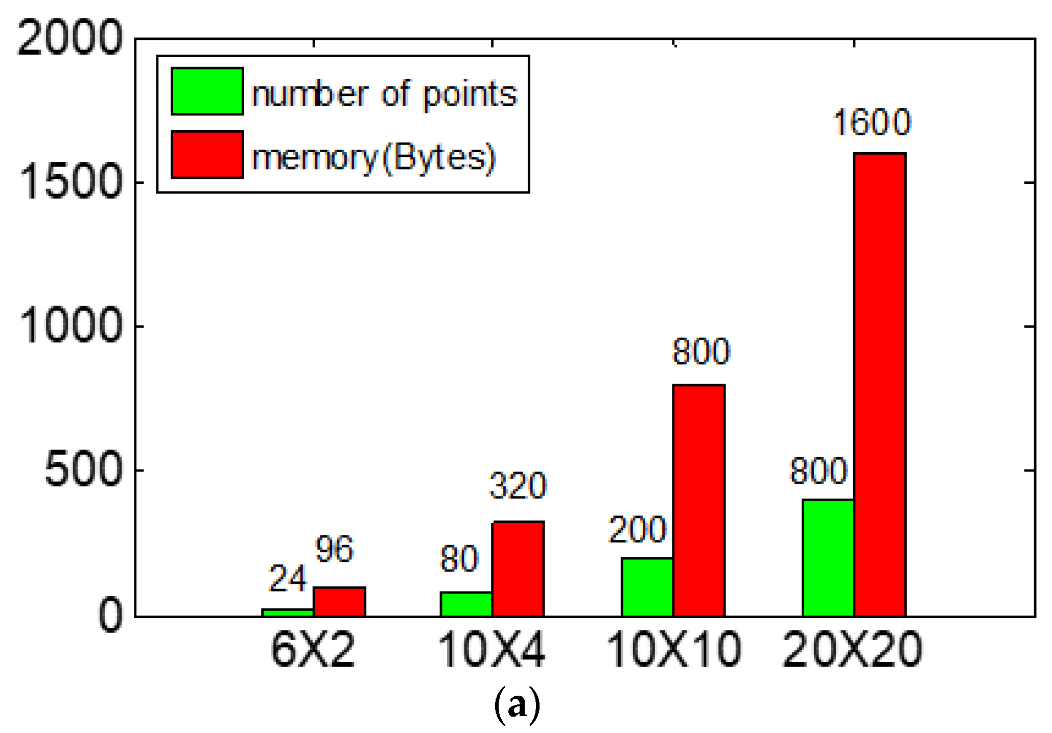
The only required flux-linkage-map information is a 6 × 2 LUT, which can be acquired via simple experimental self-commissioning procedures.

(b)

Three-dimensional modified linear cubic spline interpolation method (3D-MLCSIM) can extend the three-dimensional flux-linkage map to tune the accuracy as required.

(c)

The proposed online golden section searching method (GSSM) has been proven to be a faster solution with only 11 iterations to search for an optimal MTPA operating point.

The remainder of this study is organized as follows. Section 2 describes the magnetic model and MTPA control for the SynRM. In Section 3, the flux-linkage acquisition procedure with the triangle injection method is described. In Section 4, the GSSM-based MTPA search method is explained. In Section 5, the experimental results are presented. In Section 6, the conclusions, highlighting the outcomes and benefits of this study, are presented.

2. Model of the Synchronous Reluctance Machine

2.1. SynRM Model with Magnetic Saturation and Cross-Saturation Effect

In the dq-axis frame, the voltage and flux linkage equations of the SynRM are described as follows.

$$\left\{\begin{array}{l}{u}_d=R_s{i}_d+\frac{d{\psi }_d}{dt}-{\omega }_e{\psi }_q\\ u_q=R_s{i}_q+\frac{d{\psi }_q}{dt}+{\omega }_e{\psi }_d\end{array}\right.$$

(1)

The torque equation can be described as

$$T_e=1.5\mathrm{p}({\psi }_d{i}_q-{\psi }_q{i}_d)$$

(2)

Owing to the magnetic circuit saturation effect, the dq-axis flux linkage cannot continuously increase with an increase in the dq-axis current, as analyzed by FEA, as shown in Figure 1a,b. The flux linkage entered the magnetic saturation region when the dq-axis current was large enough. In addition, owing to the influence of the magnetic cross-saturation effect, the d-axis flux linkage also declines slightly with an increase in the q-axis current, and the q-axis flux linkage is subject to the same behaviors.

The FEA results of dq-axis inductance and mutual inductance as a function of the dq-axis currents, respectively. Dq-axis inductance and mutual inductance can be expressed as follows.

$$L_d(i_{\mathrm{d}},i_q)=\frac{{\psi }_d(i_{\mathrm{d}},i_q)}{i_d}$$

(3)

$$L_q(i_{\mathrm{d}},i_q)=\frac{{\psi }_q(i_{\mathrm{d}},i_q)}{i_q}$$

(4)

$$L_{dq}(i_{\mathrm{d}},i_q)=\frac{\partial {\psi }_d(i_{\mathrm{d}},i_q)}{\partial i_q}=\frac{\partial {\psi }_q(i_{\mathrm{d}},i_q)}{\partial i_d}$$

(5)

As shown in Figure 1, treating the dq-axis flux linkage and dq-axis inductance as an analytical expression is challenging. Given the strong nonlinearity of the flux linkage, the voltage equation in (1), inductance in (3)–(5), and torque equation in (2) also exhibit strong nonlinearity.

2.2. MTPA Control

For a given operating condition corresponding to a defined torque demand, the MTPA control method focuses on the minimum copper losses with maximum torque production, which has attracted increasing interest in academia and industry.

The MTPA solution was formulated to solve the copper-loss minimization problem. The superscript “*” denotes the reference value of the current in the subsequent description.

$$\left\{\begin{array}{ll}\min & R_s(i_d^{*2}+i_q^{*2})\\ s.t.& T_e^{*}=\frac{3}{2}\mathrm{p}(L_d-L_q)i_d^{*}{i}_q^{*}\end{array}\right.$$

(6)

The Lagrange multiplier applied for minimum copper loss can be described as follows.

$$H(i_d^{*},i_q^{*},\lambda )=R_s(i_d^{*2}+i_q^{*2})+\lambda [T_e^{*}-\frac{3}{2}p(L_d-L_q)i_d^{*}{i}_q^{*}]$$

(7)

$$\left\{\begin{array}{l}\frac{\partial H(i_d^{*},i_q^{*},\lambda )}{\partial i_d}=2R_s{i}_d^{*}-\lambda \frac{3}{2}\mathrm{p}((L_d-L_q)i_q^{*}+(\frac{\partial L_d}{\partial i_d}-\frac{\partial L_q}{\partial i_d})i_d^{*}{i}_q^{*})=0\\ \frac{\partial H(i_d^{*},i_q^{*},\lambda )}{\partial i_q}=2R_s{i}_q^{*}-\lambda \frac{3}{2}\mathrm{p}((L_d-L_q)i_d^{*}+(\frac{\partial L_d}{\partial i_q}-\frac{\partial L_q}{\partial i_q})i_d^{*}{i}_q^{*})=0\\ \frac{\partial H(i_d^{*},i_q^{*},\lambda )}{\partial \lambda }=T_e-\frac{3}{2}p(L_d-L_q)i_d^{*}{i}_q^{*}=0\end{array}\right..$$

(8)

By eliminating the parameter in (8).

$$\left\{\begin{array}{l}{T}_e^{*}-\frac{3}{2}p[(L_d-L_q)i_d^{*}{i}_q^{*}]=0\\ (L_d-L_q)i_d^{*2}-(L_d-L_q)i_q^{*2}+L_2{i}_d^{*2}{i}_q^{*}-L_1{i}_d^{*}{i}_q^{*2}=0\end{array}\right.$$

(9)

where $L_1=\frac{\partial L_d(i_d,i_q)}{\partial i_d}-\frac{\partial L_q(i_d,i_q)}{\partial i_d}$, $L_2=\frac{\partial L_d(i_d,i_q)}{\partial i_q}-\frac{\partial L_q(i_d,i_q)}{\partial i_q}$.

If the magnetic saturation and cross-saturation effects are neglected, it is worth observing that the MTPA mathematical relationship in (9) can be simplified as a 45° control (id* = iq* control). However, the issues related to MTPA control are as follows:

(a)

Traditional motor parameters, such as the dq-axis inductance and flux linkage, are considered constant and independent of the motor operating point. However, these parameters change with the input current under actual operating conditions.

(b)

Considering variable inductance, the dq-axis current along the MTPA curve can be obtained by solving (9) with a given torque, as discussed in [19,20,21].

$$\left\{\begin{array}{l}{i}_d^{*}=\frac{\mathrm{S}-\sqrt{{\mathrm{S}}^2-4\mathrm{T}}}{2}\\ i_q^{*}=\frac{\mathrm{S}+\sqrt{{\mathrm{S}}^2-4\mathrm{T}}}{2}\end{array}\right.$$

(10)

In (10), the MTPA curve consists of partial differential equations, LUTs, and square root operation, which is a challenging task implemented directly in MCU.

(c)

The LUT method is commonly used, and these LUTs tend to be large with large memory because it is necessary to create separate MTPA tables based on inductance variation. Estimating MTPA with parameter variation requires considerable posting fitting work, which is time-consuming.

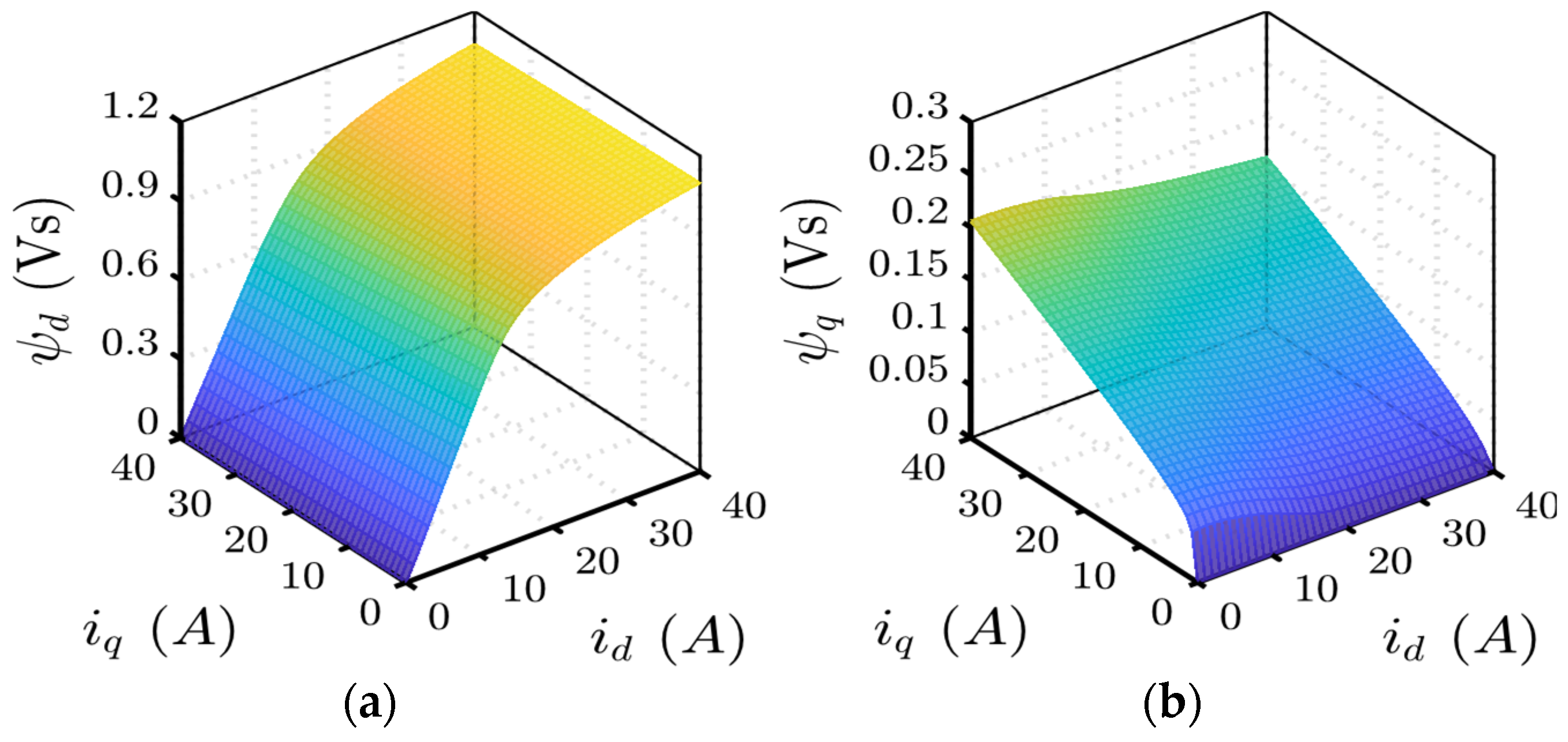
3. Flux Linkage Map Self-Identification

Many types of inductance and flux linkage self-commissioning methods are proposed in the literature [5,6,7,8,9,10,11], which can be divided primarily into dynamic and standstill methods. The method to correctly obtain the experimental values of flux linkage and inductance in this study is not in the scope of discussion. A detailed and time-efficient triangle current injection is discussed in [7]. The dq-axis flux linkage can be calculated from (11). The experimental results were compared with the FEA results, and the maximum normalized dq-axis flux differences are 2.8% and 8.3%, as shown in Figure 2a,b.

$$\left\{\begin{array}{l}{\psi }_d(i_d,i_q)=\frac{u_q-R_s{i}_q}{{\omega }_e}\\ {\psi }_q(i_d,i_q)=-\frac{u_d-R_s{i}_d}{{\omega }_e}\end{array}\right.$$

(11)

More accurate steps can be added to increase the accuracy of the operating point, as described in [7,8], which can be used to expand the number of points for the LUT. However, an increase in the number of operating points prolongs the total time of the self-commissioning procedure and occupies more memory resources in the microcontroller. For example, a 61 × 61 single float data LUT occupies approximately 15 kBytes, whereas a 21 × 21 single float data LUT occupies about 1.76 kB. If the dq-axis flux-linkage LUTs are considered, then the memory is doubled. To shorten the memory usage, in our case, only a 6 × 2 single float data LUT (marked as ◆ in Figure 2) was used, with only 48 Bytes of memory usage.

4. Proposed GSSM for MTPA

A golden section search method was proposed to realize a highly accurate flux-linkage LUT and MTPA based on a simple dq-axis 6 × 2 flux-linkage LUT.

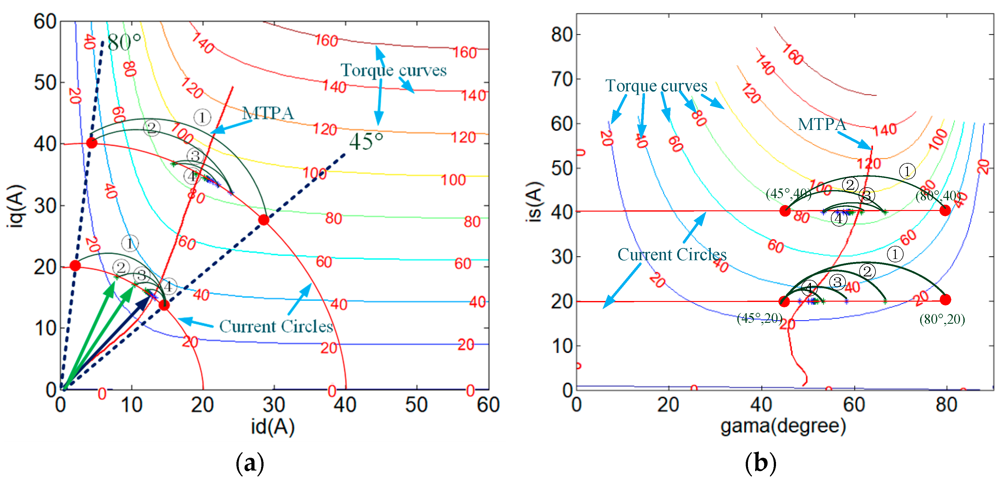
4.1. MTPA Curve on Polar Coordinates

MTPA is defined as the maximum torque to current ratio control:

$${\left.f\left(i_d,i_q\right)\right|}_{MTPA}=\frac{T_e}{i_s}=\frac{1.5\mathrm{p}({\psi }_d{i}_q-{\psi }_q{i}_d)}{\sqrt{i_d^2+i_q^2}}$$

(12)

The torque overcurrent can be defined as an MTPA function, and the MTPA curve is used to determine the optimal dq-axis current to satisfy the maximum MTPA function. This simplifies the calculations. The function can be redefined as follows.

$${\left.find\left(i_d^{*},i_q^{*}\right)\to f\left(i_d,i_q\right)\right|}_{\max }=\frac{{\psi }_d{i}_q-{\psi }_q{i}_d}{\sqrt{i_d^2+i_q^2}}$$

(13)

If the above expression is converted to polar coordination through (14),

$$\left\{\begin{array}{l}{i}_d=i_s\cos \gamma \\ i_q=i_s\sin \gamma \end{array}\right.$$

(14)

Then, the MTPA function can be expressed as follows.

$${\left.f\left(\gamma \right)\right|}_{\max }={\psi }_d(i_s^{*}\cos \gamma ,i_s^{*}\sin \gamma )\sin \gamma -{\psi }_q(i_s^{*}\cos \gamma ,i_s^{*}\sin \gamma )\cos \gamma$$

(15)

The problem can be restated to find the optimal angle γ at the maximum value of the function f(γ) with different given currents.

Compared with the (12) dq-axis current, the proposed new function (15) on polar coordination, only one parameter, optimal angle γ, should be determined. The dq-axis flux linkage LUTs ${\psi }_{\mathrm{d}}(i_{\mathrm{s}}^{\mathrm{*}}\mathrm{c}\mathrm{o}\mathrm{s}\mathsf{\gamma },i_{\mathrm{s}}^{\mathrm{*}}\mathrm{s}\mathrm{i}\mathrm{n}\mathsf{\gamma })$ and ${\psi }_{\mathrm{q}}(i_{\mathrm{s}}^{\mathrm{*}}\mathrm{c}\mathrm{o}\mathrm{s}\mathsf{\gamma },i_{\mathrm{s}}^{\mathrm{*}}\mathrm{s}\mathrm{i}\mathrm{n}\mathsf{\gamma })$ in polar coordinates are difficult to handle and require interpolation and trigonometric operations, which require a long execution time.

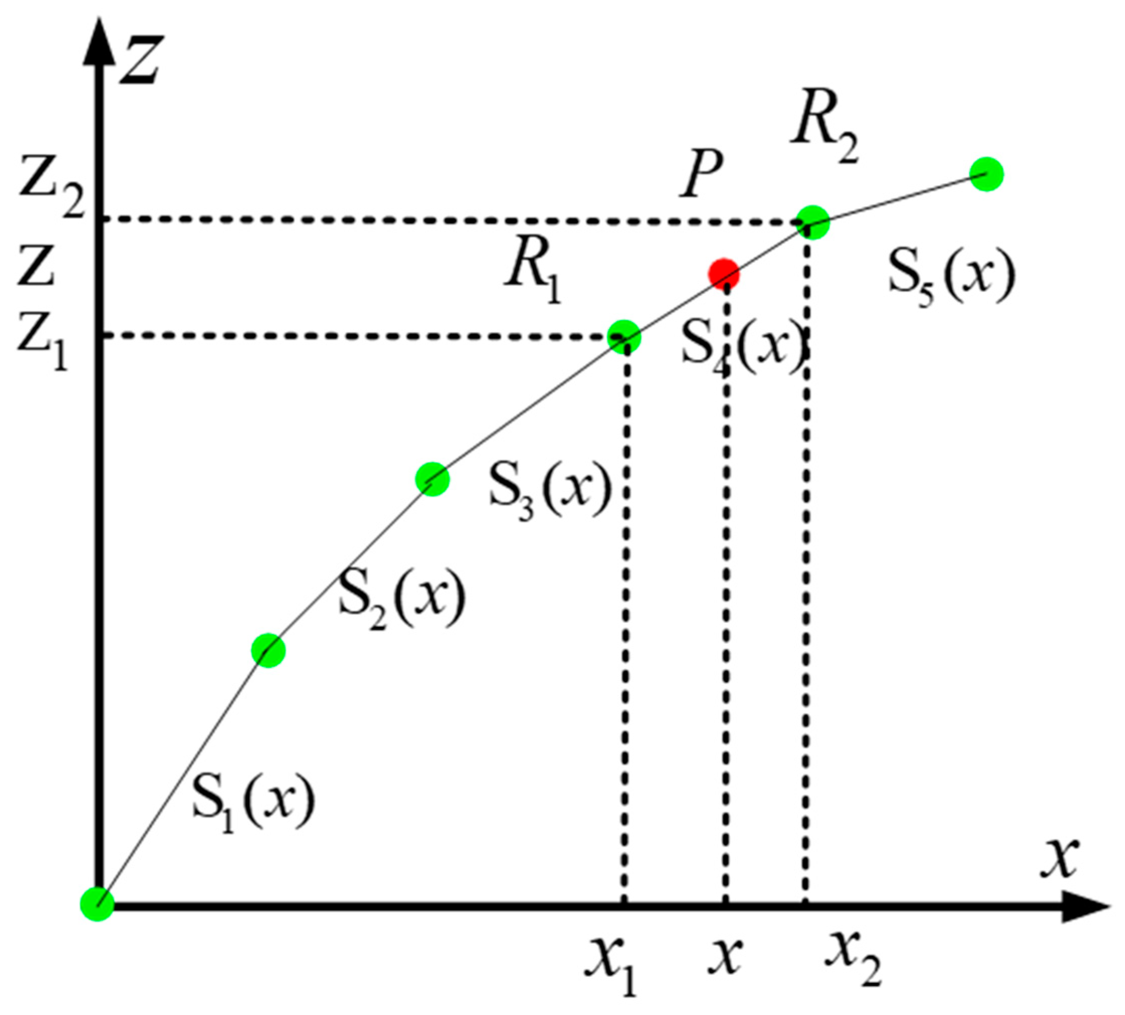
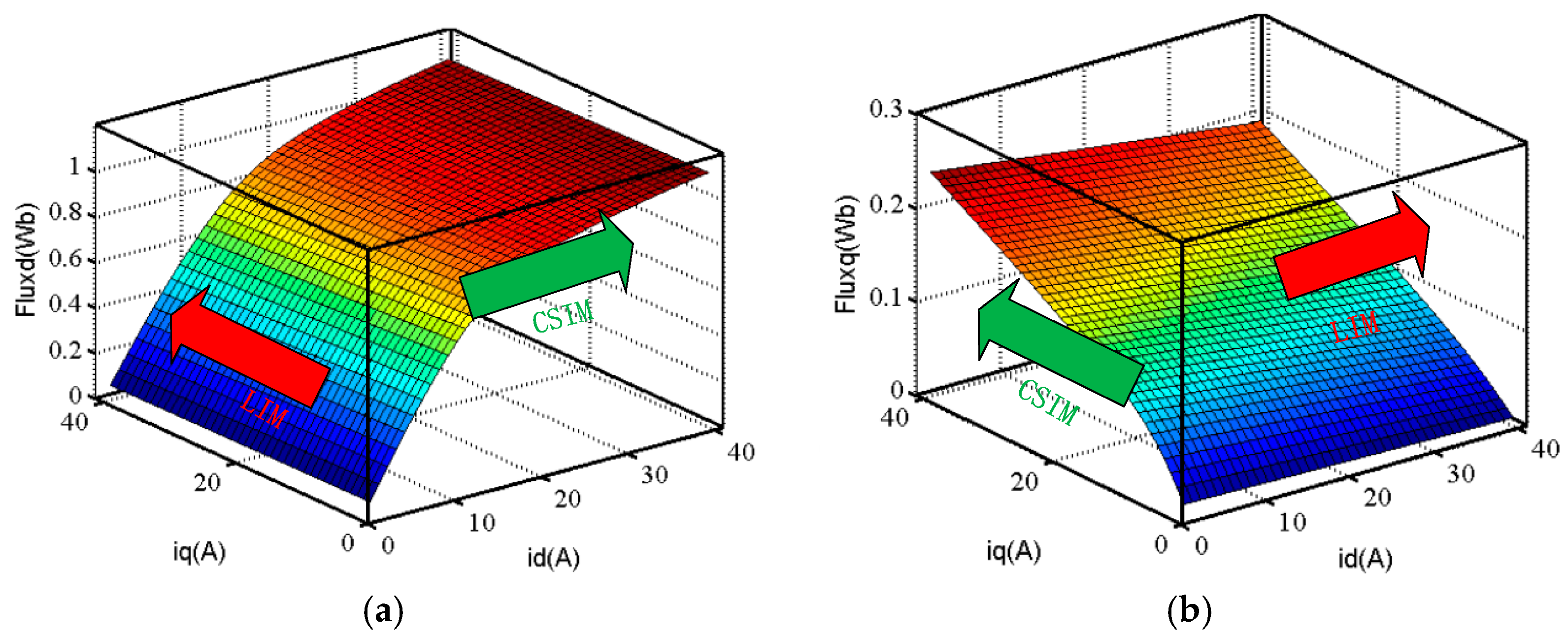
4.2. Modified Linear Cubic Spline Interpolation Method for Magnetic and Cross Saturation Effect

To decrease the measurement time and memory occupation, two 6 × 2 single float data LUTs (dq-axis flux-linkage) with averaged values from the experimental measurements in Figure 2 were used in practice. In this case, two 6 × 2 LUTs can only be divided into four two-dimensional LUTs. As in Figure 3, LUT1 and LUT3 only consider the effect of magnetic saturation, whereas LUT2 and LUT4 consider the impact of strong cross saturation.

It should be noted that magnetic saturation exhibits a highly nonlinear characteristic, whereas the effect of cross-saturation is less. The hybrid interpolation method can be applied to reduce the calculations and memory occupation as follows:

• The d-axis flux-linkage LUT was interpolated using the cubic spline interpolation method (CSIM) along the d-axis current input.
• The q-axis flux-linkage LUT was interpolated using the cubic spline interpolation method (CSIM) along the q-axis current input.
• The d-axis flux-linkage LUT was interpolated using the linear interpolation method (LIM) along the q-axis current input.
• The q-axis flux-linkage LUT was interpolated using the linear interpolation method (LIM) along the d-axis current input.

The proposed hybrid interpolation method is referred to as 3D-MLCSIM.

The d-axis flux linkage is detailed as an example. As shown in Figure 4a, the blue points denote the four known points listed as Q11 = z(x₁,y₁), Q12 = z(x₁,y₂), Q21 = z(x₂,y₁), and Q22 = z(x₂,y₂), while the red points denote unknown points P(x_p,y_p). If a value is required from the unknown function z = f(x,y) at point P(x_p,y_p), 3D-MLCSIM is expressed in the following steps.

Step 1. Linear interpolation is used in the y direction in Figure 4b

$$\left\{\begin{array}{l}f({\mathrm{R}}_1)\approx \frac{y_2-y_{\mathrm{p}}}{y_2-y_1}f(Q_{11})+\frac{y_{\mathrm{p}}-y_1}{y_2-y_1}f(Q_{21})\\ f({\mathrm{R}}_2)\approx \frac{y_2-y_{\mathrm{p}}}{y_2-y_1}f(Q_{12})+\frac{y_{\mathrm{p}}-y_1}{y_2-y_1}f(Q_{22})\end{array}\right.$$

(16)

Step 2. cubic spline interpolation is used in the x direction in Figure 4c.

Considering that x_p is within the range of [x_j,x_j + 1], cubic spline interpolation is used to obtain flux-linkage results at given points, and the online solution is provided in Appendix A, which is obtained via LU factorization and iterative method.

$$\begin{array}{l}\mathrm{z}(P(x_p,y_p))\approx \frac{{(x_{j+1}-x_p)}^3}{6(x_{j+1}-x_j)}{M}_j+\frac{{(x_p-x_j)}^3}{6(x_{j+1}-x_j)}{M}_{j+1}+\mathrm{A}+\mathrm{B}\\ \mathrm{A}=(f({\mathrm{R}}_1)-\frac{M_j}{6}{(x_{j+1}-x_j)}^2)\frac{x_2-x_p}{(x_{j+1}-x_j)}\\ \mathrm{B}=(f({\mathrm{R}}_2)-\frac{M_{j+1}}{6}{(x_{j+1}-x_j)}^2)\frac{x_p-x_j}{(x_{j+1}-x_j)}\end{array}$$

(17)

Figure 5 shows the simulation results after the interpolation operation. The direction of the green arrow corresponds to a LIM, whereas the red arrow shows the CSIM.

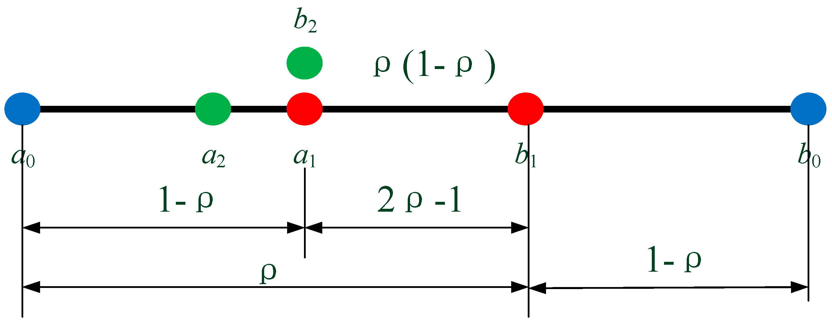
4.3. Golden Section Searching for MTPA

The GSSM is an interval contraction method, which gradually reduces the interval containing the optimal solution until the interval length is zero.

For example, to determine the minimum value point of function f(x) in the interval [a,b], any two points x₁ and x₂ can be selected within the range of [a,b] by comparing the function value or derivative value of function f(x) at these two points. Part of the interval [a,x₁] or [x₂,b] is removed to decrease the length of the search interval. The method continues to iterate until the interval shrinks to one point or the interval length is less than a given accuracy ε. The optimal x is determined.

2ρ − 1 = ρ(1 − ρ)

(18)

The interval contraction is repeated as [a₀,b₀] → [a₀,b₁] → [a₂,b₁], as shown in Figure 6. The mathematical relationship is provided in (18). By solving (18), the interval compression ratio ρ corresponds to 0.618. In particular, a₁ and b₁ denote the golden section point of the interval [a₀,b₀], whereas a₂ and b₂ denote the golden section point of the interval [a₀,b₁].

The function f(γ) in (15) exhibits the following characteristics. The function equation f(γ) is a unimodal function with respect to angle γ. The unimodal function refers to the function f(γ) on the interval [a,b], which exists only at one point ${\gamma }^{\mathrm{*}}$ within the interval [a,b]. Thus, the function f(γ) increases (decreases) strictly monotonically on [a,${\gamma }^{\mathrm{*}}$] and decreases (increases) strictly monotonically on [${\gamma }^{\mathrm{*}}$,b].

Figure 7 shows the flow chart of the entire GSSM. The detailed search algorithm is described in the following steps.

Step 1 Initialize the interval [a,b] as random [a₀,b₀] and set the search error ε > 0. In this particular case, the interval upper and lower limits, a₀ and b₀, are set as 45° and 80°, respectively, and the error limit ε is set as 0.1°. It is noted that the MTPA angle is within [45°,80°] in all the current operating points. The random initial interval limits of 45° and 80° can be selected as the maximum interval range to cover all optimal MTPA angles. Since the torque is 0 N.m, the dq-axis current reference usually equals the 45° MTPA angle.

Step 2 Define two golden section checkpoints: γ₁ = a + 0.382 (b − a) and γ₂ = a + 0.618 (b − a).

Step 3 Calculate four flux-linkage values at given γ₁ and γ₂ using 3D-MLCSIM Ψ_d1 Ψ_q1 Ψ_d2 Ψ_q2; further, calculate f(γ₁) f(γ₂) using Equation (15) and divide the search interval into two cases:

• If f (γ₁) ≤ f (γ₂), then the optimal solution (i.e., γ*) when the function takes the maximum value can only be located in the interval (γ₁,b). In this case, a is denoted as γ_1, and b remains unchanged. Additionally, γ₁ is assigned as γ₂, and new γ₂ is calculated using the expression γ₂ = a + 0.618(b − a). Furthermore, update f(γ₂) using (15).
• If f (γ₁) > f (γ₂), then the optimal solution (i.e., γ*) can only be located in the interval [a,γ₂). In this case, a remains unchanged, b is assigned as γ₂, and γ₂ is assigned as γ₁. Calculate new γ₁ using the formula γ₁ = a + 0.382 (b − a) and update f (γ₁) using (15).

Step 4 Calculate the new interval (b − a) in Step 3: if the interval length is less than the searching error ε, stop the iteration and return to Step 5; otherwise, return to Step 3.

Step 5 Use the midpoint γ* = (a + b)/2 of the last interval as the approximate optimal solution and obtain MTPA dq-axis current.

The Interval compression ratio ρ is 0.618. The accuracy is defined as follows.

$$(b_0-a_0){\rho }^N<\epsilon$$

(19)

The final iterations are expressed as follows.

$$N>\log \frac{\epsilon }{(b_0-a_0)}/\log (\rho )$$

(20)

The proposed method has the following characteristics listed as follows.

(a)

The proposed online method does not require curve fitting. Only limited information is required, and it is easier to access these using self-identification methods.

(b)

Function equation f(γ) is a unimodal function, and only one maximum value is determined within the range [45° to 80°].

(c)

If the search error ε is set to 0.1°, then the maximum iteration can be calculated from (20) as 11. If the searching error ε is set to 0.5°, then the maximum number of iterations is 8.

(d)

3D-MLCSIM can be used only once during each iteration to save the calculation.

(e)

The flux linkage and torque values can be calculated simultaneously for the benefit of the high-performance control method, for example, sensorless control, which relies on the parameters.

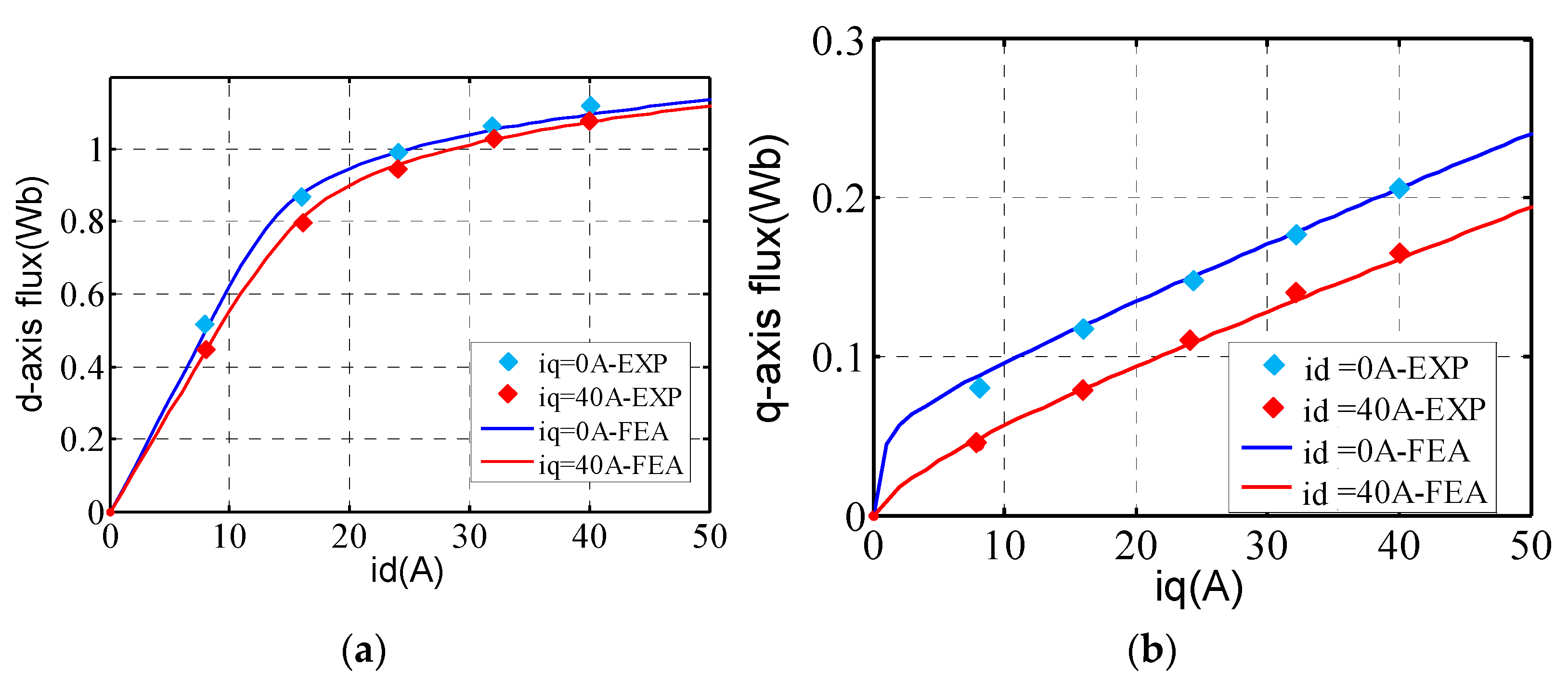
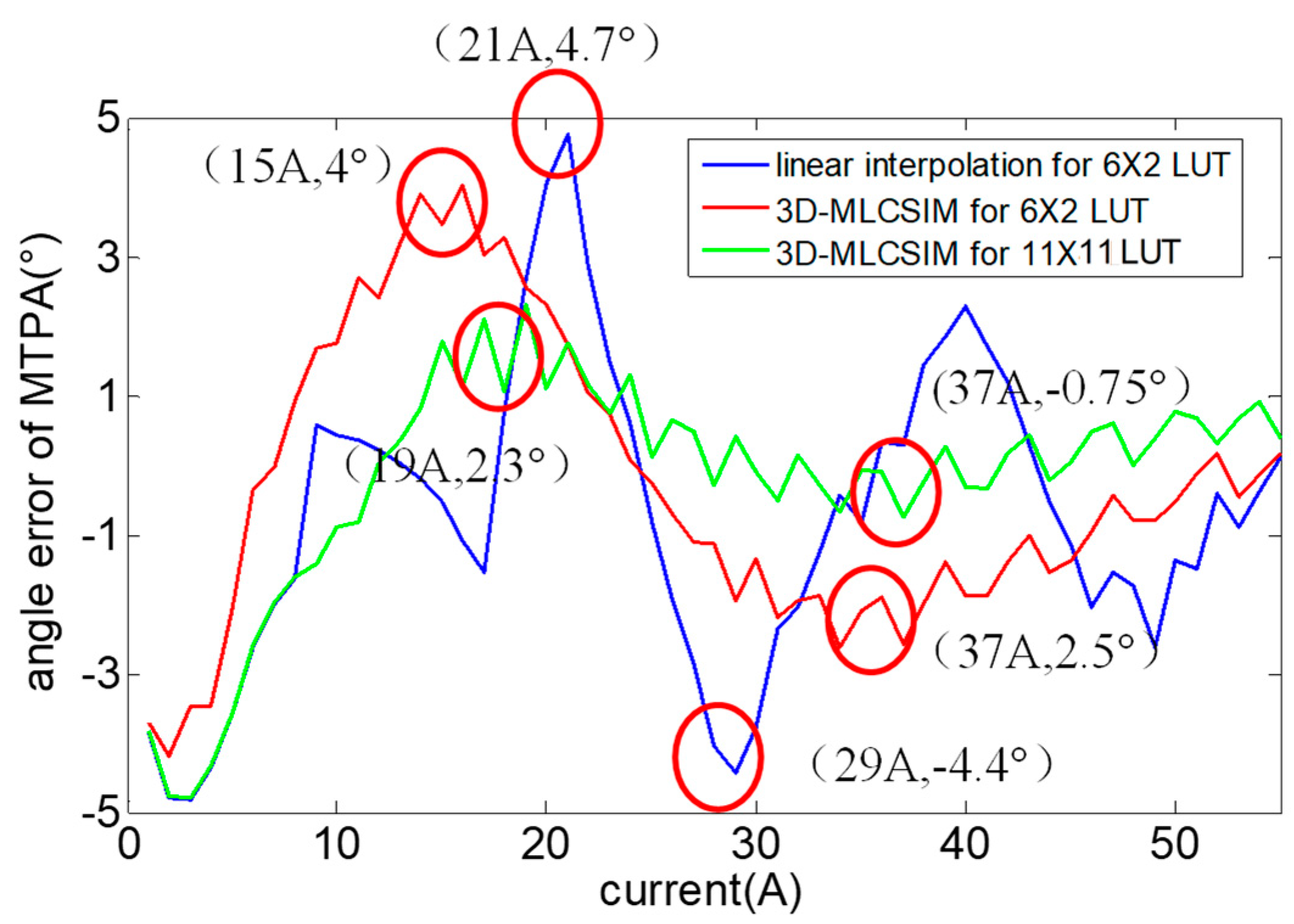
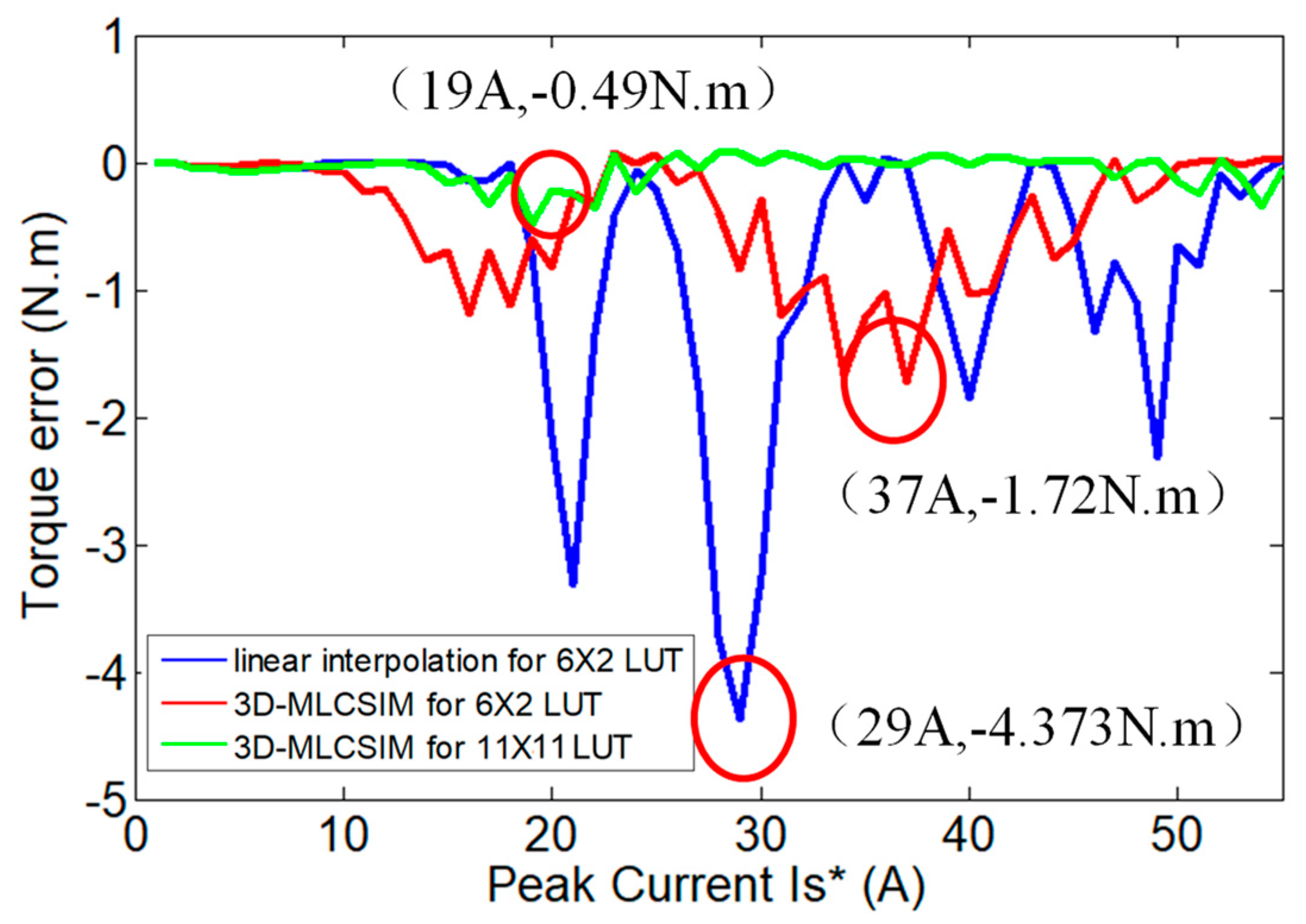
5. Experimental Results

Figure 8a,b show the experimental test bench and DSP-based controller. The machine under test (SynRM 15 Kw prototype) is on the left-hand side, and the parameters are listed in

Table 1. 15-Kw SynRel machine parameters.

Synrm Parameters	Values	Units	Parameters	Values	Units
Rated power	15	Kw	Shaft diameter	60	mm
Rated torque	96	Nm	Stack length	205	mm
Rated speed	1500	Rpm	slots	48
Rated phase current	33	A-RMS	poles	4
Rated phase voltage	210	V-RMS	Tooth width	5	mm
Stator outer diameter	260	mm	Slot height	20.3	mm
Rotor outer diameter	169	mm	Air gap	0.5	mm

. A torque transducer (Kistler 4503A200WA2B100, Winterthur, Switzerland) is mounted between the two shafts. The induction machine on the right-hand side can be used as a prime mover or dynamometer. The speed and angle were measured using a resolver (TAMAGAWA, 52AXU7102D, Nagano, Japan, TMS320F28377, DSP, Dallas, TX, USA). Digital signal processing (DSP Type: TMS320F28377, Dallas, TX, USA) was used as the core device for the controller. An RS485 communication cable was used to obtain real-time data from the DSP. The phase currents were sampled by three current sensors (Type: LEM), the DC-link voltage was also sampled, and all entered the DSP’s analog-to-digital (AD) channels.

Table 2. GSSM at 30 A.

i	a	b	γ1	γ2	f(γ1)	f(γ2)	γ2 − γ1
1	45.00	80.00	58.37	66.63	0.6343	0.5709	8.26
2	45.00	66.63	53.26	58.37	0.6390	0.6343	5.11
3	45.00	58.37	50.11	53.26	0.6300	0.6390	3.16
4	50.11	58.37	53.26	55.21	0.6390	0.6401	1.95
5	53.26	58.37	55.21	56.42	0.6401	0.6389	1.21
6	53.26	56.42	54.47	55.21	0.6399	0.6401	0.75
7	54.47	56.42	55.21	55.67	0.6401	0.6399	0.46
8	54.47	55.67	54.93	55.21	0.6401	0.6401	0.28
9	54.93	55.67	55.21	55.39	0.6401	0.6401	0.18
10	55.21	55.67	55.39	55.50	0.6401	0.6401	0.11
11	55.21	55.50	55.32	55.39	0.6401	0.6401	0.07

lists the convergence procedure of the proposed GSSM at 30 A current input. As shown in Table 2, the total iterations at 30 A are 10. Considering the search accuracy ε as 0.1°, γ₁ or γ₂, a or b, f(γ₁), or f(γ₂), only one of the values is updated at each iteration, whereas the other values maintain the value from the previous step. Each search interval (γ₂ − γ₁) shrinks by 0.618, as shown in (19) and (20). The final steps required are fixed as $\log \frac{\epsilon }{(b_0-a_0)}/\log (\rho )$. The final γ* is selected as 55.36°.

The 20 A and 40 A peak currents are selected as inputs for the GSSM to show the algorithm’s search process. Figure 9a,b show the algorithm convergence process in the dq-axis current and polar coordinate planes, respectively. Figure 9a is torque are the torque, current, and MTPA curves in the dq-axis current plane. The dq-axis current plane is well known to describe the torque, current constraint, voltage constraint, MTPA, etc., as discussed in [14,15,16,17,18]. The red quarter circle represents the amplitude of a given current. We selected 20 A and 40 A as case studies. A series of curves with color contour lines represent torque sensor values with 20 N.m as a step. The red solid line denotes the MTPA experimental curve. The steps of the interval shrinking are denoted by ①–④.

Figure 9b is the polar coordination form of Figure 9a, using $\left\{\begin{array}{l}{i}_d^{*}=i_s^{*}\cos \gamma \\ i_q^{*}=i_s^{*}\sin \gamma \end{array}\right.$. The proposed search algorithm can continuously shrink the interval for optimization, and it finally converges to the MTPA curve.

Figure 10 shows the data relationship between the MTPA angle error and current amplitude using different interpolation algorithms. The experimental MTPA procedure is: by providing a constant current, the current angle changes slightly until the maximum torque point is determined via the torque sensor. The current angle we find is defined as ${\Upsilon }_{\exp ,\mathrm{MTPA}}$, and the MTPA we obtained from GSSM is defined as ${\Upsilon }_{GSSM,\mathrm{MTPA}}$.

The MTPA angle error in Figure 10 is calculated as:

$$Er{r}_{\Upsilon }={\Upsilon }_{\exp ,\mathrm{MTPA}}-{\Upsilon }_{GSSM,\mathrm{MTPA}}$$

(21)

Herein, the blue line denotes the MTPA observation angle error curve constructed by the linear interpolation method under 6 × 2 LUTs (Method I), the red line indicates the MTPA observation error curve constructed by 3D-MLCSIM under 6 × 2 LUTs (Method II), and the green line denotes the MTPA observation error curve constructed by 3D-MLCSIM under 11 × 11 LUTs (Method III). As shown in Figure 10, the maximum MTPA angle error points approximately corresponded to 4.7° at 21 A for Method I, 4° at 15 A for Method II, and 2.3° at 19 A for Method III.

Figure 11 depicts the torque error in MTPA from three methods, and the maximum torque error points approximately located at −4.37 N.m at 29 A for Method I, −1.72 N.m at 37 A for Method II, and −0.49 N.m at 19 A for Method III.

The experimental torque from the torque sensor is calculated while using ${\Upsilon }_{\exp ,\mathrm{MTPA}}$ with different currents. The estimation torque is calculated using torque equation $T_e=1.5\mathrm{p}({\psi }_d{i}_q-{\psi }_q{i}_d)$ from ${\Upsilon }_{GSSM,\mathrm{MTPA}}$. The torque error in Figure 11 is calculated as

$$Er{r}_{Te}=T_e({\Upsilon }_{\exp ,\mathrm{MTPA}})-T_e({\Upsilon }_{GSSM,\mathrm{MTPA}})$$

(22)

Method III presents higher accuracy with larger LUTs. In Method II, it should be noted that most of the error peaks are close to the range from 15 A to 20 A, which approximately corresponds to 1/3 to 2/5 of the rated current. Given the low current range, the motor copper loss is not very high, and the error does not decrease efficiency. However, in the higher current range, Method I still exhibited higher angle error and lost around −4.3 N.m available torque, denoted as −4.4° at 29 A. Compared with Method I, Method II and Method III exhibited better accuracy with maximum errors of 2.5° and −0.75°, respectively.

The proposed method has been tested under acceleration dynamic conditions without load and with rated load, as shown in Figure 12a,b, respectively. The 3D-MLCSIM under 6 × 2 LUTs combined with GSSM is used for testing. It can be seen that the proposed method shows quite good dynamic performance covering from no load to full load.

As shown in Figure 13a–c, different sizes of dq-axis flux-linkage LUTs were compared regarding memory occupation, calculation time, and time duration for the self-commissioning procedure. As shown in Figure 13a, given the single float format of data saved in DSP memory, the 6 × 2 dq-axis flux-linkage LUT only occupied 96 Bytes, as compared with 1.6 k Bytes for the 20 × 20 dq-axis flux-linkage LUT. The calculation time for the proposed 3D-MLCSIM was compared with that of the well-known bilinear interpolation method, and the results are shown in Figure 13b. The proposed interpolation time in FOC was approximately four times that of the bilinear interpolation method because the proposed interpolation exhibited higher computational complexity. The maximum MTPA error changed from 4° to 0.4° when the size of the table increased from a 6 × 2 LUT to a 20 × 20 LUT. However, the 6 × 2 LUT exhibited good agreement in the MTPA curve under most operating conditions, as shown in Figure 13c, which can be accepted in some low-cost MCUs. The two self-commissioning methods, which are denoted as ‘triangle-pulses’ in [7] and ‘square pulses’ in [8] for flux-linkage LUTs, were selected as the case study; the ‘three-triangle-pulses’ obtained the exact size of the LUT faster than the ‘three-pulse’. When the LUT was chosen as 6 × 2, only 0.4 min was required to conduct all possible points reported in [7]. The calculation time of the GSSM did not change significantly with the increasing size of the LUT because the fixed 11 iterations were used for every operating point. The total time for fast self-commissioning with a 6 × 2 dq-axis flux-linkage LUT and MTPA searching was only 31.6 s.

6. Conclusions

The study proposed an automated MTPA identification method for SynRMs with limited flux linkage information. A limited dq-axis flux-linkage map, a 6 × 2 LUT, was obtained by applying symmetric triangle pulses in the self-commissioning stage. The hybrid interpolation method 3D-MLCSIM was used to extend the data. Golden section searching was proposed to obtain the MTPA curve. The advantage of the proposed method was observed in the high accuracy of MTPA curves with less calculation time and low memory occupation under 11 iterations. This corresponds to a suitable and promising solution for specific low-cost microcontroller applications, such as household appliances and other industrial applications.

References

1. Odhano, S.A.; Pescetto, P.; Awan, H.A.A.; Hinkkanen, M.; Pellegrino, G.; Bojoi, R. Parameter identification and self-commissioning in AC motor drives: A technology status review. IEEE Trans. Power Electron. 2018, 34, 3603–3614. [Google Scholar] [CrossRef]
2. Miao, Y.; Ge, H.; Preindl, M.; Ye, J.; Cheng, B.; Emadi, A. MTPA fitting and torque estimation technique based on a new flux-linkage model for interior-permanent-magnet synchronous machines. IEEE Trans. Ind. Appl. 2017, 53, 5451–5460. [Google Scholar] [CrossRef]
3. Rabiei, A.; Thiringer, T.; Alatalo, M.; Grunditz, E.A. Improved maximum-torque-per-ampere algorithm accounting for core saturation, cross-coupling effect, and temperature for a PMSM intended for vehicular applications. IEEE Trans. Transp. Electrif. 2016, 2, 150–159. [Google Scholar] [CrossRef]
4. Bedetti, N.; Calligaro, S.; Petrella, R. Stand-still self-identification of flux characteristics for synchronous reluctance machines using novel saturation approximating function and multiple linear regression. IEEE Trans. Ind. Appl. 2016, 52, 3083–3092. [Google Scholar] [CrossRef]
5. Stumberger, B.; Stumberger, G.; Dolinar, D.; Hamler, A.; Trlep, M. Evaluation of saturation and cross-magnetization effects in interior permanent-magnet synchronous motor. IEEE Trans. Ind. Appl. 2003, 39, 1264–1271. [Google Scholar] [CrossRef]
6. Hinkkanen, M.; Pescetto, P.; Molsa, E.; Saarakkala, S.E.; Pellegrino, G.; Bojoi, R. Sensorless self-commissioning of synchronous reluctance motors at standstill without rotor locking. IEEE Trans. Ind. Appl. 2016, 53, 2120–2129. [Google Scholar] [CrossRef]
7. Varvolik, V.; Wang, S.; Prystupa, D.; Buticchi, G.; Peresada, S.; Galea, M.; Bozhko, S. Fast Experimental Magnetic Model Identification for Synchronous Reluctance Motor Drives. Energies 2022, 15, 2207. [Google Scholar] [CrossRef]
8. Armando, E.; Bojoi, R.I.; Guglielmi, P.; Pellegrino, G.; Pastorelli, M. Experimental identification of the magnetic model of synchronous machines. IEEE Trans. Ind. Appl. 2013, 49, 2116–2125. [Google Scholar] [CrossRef]
9. Hall, S.; Márquez-Fernández, F.J.; Alaküla, M. Dynamic magnetic model identification of permanent magnet synchronous machines. IEEE Trans. Eng. Convers. 2017, 32, 1367–1375. [Google Scholar] [CrossRef]
10. Wiedemann, S.; Hall, S.; Kennel, R.M.; Alakula, M. Dynamic Testing Characterization of a Synchronous Reluctance Machine. IEEE Trans. Ind. Appl. 2017, 54, 1370–1378. [Google Scholar] [CrossRef]
11. Pellegrino, G.; Boazzo, B.; Jahns, T.M. Magnetic model self-identification for PM synchronous machine drives. IEEE Trans. Ind. Appl. 2014, 51, 2246–2254. [Google Scholar] [CrossRef]
12. Kim, S.; Yoon, Y.D.; Sul, S.K.; Ide, K. Maximum torque per ampere (MTPA) control of an IPM machine based on signal injection considering inductance saturation. IEEE Trans. Power Electron. 2012, 28, 488–497. [Google Scholar] [CrossRef]
13. Lai, C.; Feng, G.; Tjong, J.; Kar, N.C. Direct calculation of maximum-torque-per-ampere angle for interior PMSM control using measured speed harmonic. IEEE Trans. Power Electron. 2018, 33, 9744–9752. [Google Scholar] [CrossRef]
14. Bolognani, S.; Petrella, R.; Prearo, A.; Sgarbossa, L. Automatic tracking of MTPA trajectory in IPM motor drives based on AC current injection. IEEE Trans. Ind. Appl. 2010, 47, 105–114. [Google Scholar] [CrossRef]
15. Liu, G.; Wang, J.; Zhao, W.; Chen, Q. A novel MTPA control strategy for IPMSM drives by space vector signal injection. IEEE Trans. Ind. Electron. 2017, 64, 9243–9252. [Google Scholar] [CrossRef]
16. Sun, T.; Wang, J.; Chen, X. Maximum torque per ampere (MTPA) control for interior permanent magnet synchronous machine drives based on virtual signal injection. IEEE Trans. Power Electron. 2014, 30, 5036–5045. [Google Scholar] [CrossRef]
17. Zhao, J.; Liu, W.; Tan, B. Research of maximum ratio of torque to current control method for PMSM based on least square support vector machines. In Proceedings of the 2010 International Conference on Electrical and Control Engineering, Wuhan, China, 25–27 June 2010; pp. 1623–1628. [Google Scholar]
18. Lin, F.J.; Liu, Y.T.; Yu, W.A. Power perturbation based MTPA with an online tuning speed controller for an IPMSM drive system. IEEE Trans. Ind. Electron. 2017, 65, 3677–3687. [Google Scholar] [CrossRef]
19. Pervin, S.; Siri, Z.; Uddin, M.N. Newton-Raphson based computation of i d in the field weakening region of IPM motor incorporating the stator resistance to improve the performance. In Proceedings of the 2012 IEEE Industry Applications Society Annual Meeting, Las Vegas, NV, USA, 7–11 October 2012; pp. 1–6. [Google Scholar]
20. Wang, S.; Kang, J.; Degano, M.; Galassini, A.; Gerada, C. An Accurate Wide-speed Range Control Method of IPMSM Considering Resistive Voltage Drop and Magnetic Saturation. IEEE Trans. Ind. Electron. 2019, 67, 2630–2641. [Google Scholar] [CrossRef]
21. Dianov, A.; Tinazzi, F.; Calligaro, S.; Bolognani, S. Review and classification of MTPA control algorithms for synchronous motors. IEEE Trans. Power Electron. 2021, 37, 3990–4007. [Google Scholar] [CrossRef]
22. Zhou, J.; Xiao, X.; Wang, Z.; Lu, H.; Chai, J.; Zhang, M. Accurate MTPA strategy of PMSM considering cross saturation effect based on full-flux-linkage model. In Proceedings of the 2022 IEEE Energy Conversion Congress and Exposition (ECCE), Detroit, MI, USA, 9–13 October 2022; pp. 1–5. [Google Scholar]
23. Mahmud, M.H.; Wu, Y.; Zhao, Y. Extremum seeking-based optimum reference flux searching for direct torque control of interior permanent magnet synchronous motors. IEEE Trans. Transp. Electrif. 2019, 6, 41–51. [Google Scholar] [CrossRef]
Figure 1. FEA results of flux-linkage maps for 15 kW SynRM prototype: (a) d-axis flux linkage; (b) q-axis flux linkage.
Machines 12 00096 g001
Figure 2. Experimental flux-linkage maps: (a) d-axis flux linkage; (b) q-axis flux linkage.
Machines 12 00096 g002
Figure 3. Sample points relationship: (a) d-axis flux-linkage 6 × 2 LUT; (b) q-axis flux-linkage 6 × 2 LUT.
Machines 12 00096 g003
Figure 4. Proposed interpolation methods: (a) sampling points of d-axis flux linkage; (b) projection of data in x–y axis; (c) projection of data in x–z axis.
Machines 12 00096 g004
Figure 5. Expansion of the flux linkage 6 × 2 LUTs using 3D-MLCSIM: (a) d-axis flux-linkage; (b) q-axis flux-linkage.
Machines 12 00096 g005
Figure 6. Golden Section interval.
Machines 12 00096 g006
Figure 7. Flow chart of the proposed golden section search algorithm interval.
Machines 12 00096 g007
Figure 8. SynRM test bench: (a) test bench; (b) DSP-based controller.
Machines 12 00096 g008
Figure 9. GSSM searching procedure: (a) in dq-axis current plane; (b) in polar coordination.
Machines 12 00096 g009
Figure 10. Experimental comparison for MTPA angle error for proposed GSSM with 3D-MLCSIM in red (6 × 2 LUTs) and green (11 × 11 LUTs), and MTPA with linear interpolation in blue (6 × 2 LUTs).
Machines 12 00096 g010
Figure 11. Experimental comparison for torque error in MTPA operation for proposed GSSM with 3D-MLCSIM in red (6 × 2 LUTs) and green (11 × 11 LUTs), and with linear interpolation in blue (6 × 2 LUTs).
Machines 12 00096 g011
Figure 12. Acceleration from 100 rpm to 1500 rpm: (a) without load; (b) with rated load.
Machines 12 00096 g012
Figure 13. Experimental comparison of different LUT sizes, 6 × 2, 10 × 4, 10 × 10, and 20 × 20 of dq-axis flux-linkage: (a) memory and number of points; (b) accuracy and calculation time in FOC; (c) execution time for self-commissioning.
Machines 12 00096 g013aMachines 12 00096 g013bMachines 12 00096 g013c