Multi-Agent Reinforcement Learning Tracking Control of a Bionic Wheel-Legged Quadruped

Abstract

This paper presents a novel approach to developing control strategies for mobile robots, specifically the Pegasus, a bionic wheel-legged quadruped robot with unique chassis mechanics that enable four-wheel independent steering and diverse gaits. A multi-agent (MA) reinforcement learning (RL) controller is proposed, treating each leg as an independent agent with the goal of autonomous learning. The framework involves a multi-agent setup to model torso and leg dynamics, incorporating motion guidance optimization signal in the policy training and reward function. By doing so, we address leg schedule patterns for the complex configuration of the Pegasus, the requirement for various gaits, and the design of reward functions for MA-RL agents. Agents were trained using two variations of policy networks based on the framework, and real-world tests show promising results with easy policy transfer from simulation to the actual hardware. The proposed framework models acquired higher rewards and converged faster in training than other variants. Various experiments on the robot deployed framework showed fast response (0.8 s) under disturbance and low linear, angular velocity, and heading error, which was 2.5 cm/s, 0.06 rad/s, and 4°, respectively. Overall, the study demonstrates the feasibility of the proposed MA-RL control framework.

1. Introduction

Wheeled quadruped robots have attracted significant interest in the field of robotics in recent years. Robots possessing this configuration are capable of both quadrupedal locomotion and vehicular movement. The recent development of wheeled quadruped robots has led to a significant increase in studies focused on controlling these types of robots. There has been extensive research on legged locomotion, among which combined zero-moment point (ZMP) theory [1] and trajectory optimization based on whole-body kinematics and dynamics has a long history [2]; through this method, robots can successfully traverse tough terrain. Recently, more methods have been applied to the control of quadruped robot legged locomotion, including single rigid body modeling for the entire robot [3], inverted pendulum modeling for each individual leg [4], obtaining contact force through MPC and obtaining desired angles and generalized acceleration through WBC to achieve control over the robot [5]. For wheeled-legged composite motion, there is also a large amount of research currently, which includes composite planning based on TO and ZMP [6], as well as control based on whole-body MPC [7]. These methods can effectively integrate wheeled and legged composite motion modes to control the robot comprehensively.

While the current model-based control methods have achieved significant results, there always exists a certain level of model mismatch and violation of assumptions due to the differences between simulation and reality [8,9,10,11]. Moreover, in most cases, we tend to linearize the models, which leads to the loss of many nonlinear possibilities. For example, in paper [12], RL is used to learn the residual of dynamic models in order to approximate higher-order terms. Therefore, the application of reinforcement learning to legged robots for robot control has become a popular new approach in recent years. For instance, the authors describe a sequential collaborative agent for controlling a humanoid robot in [13]. Unlike model-based control, reinforcement learning does not require physical modeling of the robot. This method involves continuously interacting with the external environment to acquire information and learn (mostly in simulation environments) and ultimately output a deep neural network as the controller for the entire robot.

Model-free reinforcement learning (RL) has recently emerged as an alternative approach in the development of legged locomotion skills and has shown promising results on physical robots [14,15,16]. More advanced teacher-student structures have significantly improved robustness, enabling legged robots to overcome obstacles through tactile sensation [11]. There are also efforts in the model-based domain, such as the Dreamer algorithm, to achieve motion control for quadruped robots. In paper [17], the authors propose a hybrid control architecture that combines the real and simulated worlds’ strengths to achieve greater robustness, foot placement accuracy, and terrain generalization.

The evolving landscape of quadruped locomotion research is marked by a growing trend of integrating model-based and model-free approaches. Supervised [18] and unsupervised learning techniques [19,20] have been effectively employed to initialize nonlinear solvers, streamlining the optimization process. Reinforcement Learning (RL) has taken a pivotal role in both imitating [21,22] and refining [23] motion strategies derived from trajectory optimization, underscoring its versatility. Model-based methods have also evolved, now being utilized to validate the feasibility of high-level commands learned through these processes [24] and to fine-tune learned acceleration profiles [23]. This approach diverges from previous methods focused on corrective joint torques [25], moving towards a more holistic, end-to-end learning paradigm that maps reference signals to joint positions.

Recent advancements have led to the development of sophisticated policies and frameworks for quadruped robots. The integration of trajectory optimization with RL has been crucial in crafting robust policies for dynamic maneuvers like hopping and bounding [22,23]. Neural network policies, specifically designed for terrain-aware locomotion, have significantly enhanced the robots’ adaptability to unpredictable environments [24]. The Trajectory Optimization for Walking Robots (TOWR) framework represents a leap forward in planning prolonged, complex motions [18]. Conditional variational autoencoders and other function approximators are emerging as key tools for navigating obstacle-laden terrains, enabling structured and dynamic motion planning [19]. The move towards online, receding-horizon optimized trajectories has opened new avenues for adaptive locomotion planning [20]. Unified model-based and data-driven approaches have been instrumental in dynamic footstep planning, balancing stability with agility [23]. Simplified centroidal models in RL have demonstrated their efficacy through reduced computational demands and successful sim-to-real transfers, showcasing their applicability in diverse locomotion scenarios [25]. These efforts culminate in the development of hybrid control architectures that amalgamate model-based planning with neural network policies, achieving unprecedented levels of robustness and accuracy across various terrains [17]. Authors of [26] used TOWR output with a generative adversarial network in reward function to generate motions for a quadruped. These collective advancements mark a significant step toward more adaptable, robust, and efficient quadruped locomotion strategies, blending the best of both model-based and model-free worlds.

Besides foot-based motion, some works also realize wheeled motion and hybrid motion of wheel-legged robots through reinforcement learning. In [27], the authors used reinforcement learning to achieve balance control of a two-wheeled robot during rolling. Additionally, in [28], authors proposed a solution where the controller dynamically switches between wheel-based and leg-based locomotion modes based on user commands and terrain.

Our newly designed robot, Pegasus, is equipped with an independent steering system at the end of each wheel, enabling it to be operated as a vehicle [29]. Our previous work on this robot described the dynamic model, motion planner and MPC controller for quadruped locomotion and vehicular mode [29,30]. Therefore, we explore RL to develop a robot controller to control the robot’s foot and wheel movements for such a new structure.

As Pegasus does not have an onboard vision sensor, our goal is to let the RL agent learn how to operate the robot rather than how to interact with the external environment in which it is operating. For quadruped locomotion, the target is to keep the floating base balanced at every step to prevent the robot from operating in an unstable region. The motivation for a multi-agent-based setup is in three folds: first is to determine the possibility of such MA-RL control, second is to learn the dynamics of the torso, second is to learn the low-level dynamics of the actuators along with the links, and last, to enable a higher proportion of training done in hardware. As Pegasus is designed with identical actuators for different joints with similar link configurations for each leg, we model our RL controller with four cooperative agents, with the torso as its environment. The adversarial multi-agent environment can be challenging to design as quadruped is an under-actuated system where torso dynamics are the resultant actions of all the legs.

Thus, the main contribution of our work is summarized as follows:

• We propose a novel multi-agent RL framework to learn the low-level dynamics of a wheeled quadruped robot and control it by the generated model.
• The framework addresses the issue of designing reward functions for MA-RL agents when no straightforward agent-specific feedback is available.
• We also propose to add expert input signals to guide agents’ policy (in training) for well-established quadruped static and locomotive gaits. Both reward function and expert signals are implemented using a motion guidance optimizer.
• We have trained four separate controllers for Pegasus, corresponding to the four motion modes of keeping and adjusting static pose, walking, trotting, and driving.
• Two variations of the trained model have been used to demonstrate the feasibility of the motion guidance signal. Finally, one of these trained models was deployed in the robot to demonstrate its real-world application with promising results.

The remainder of this article is organized as follows: Section 2 briefly introduces the robot configuration and RL algorithms. Section 3 presents the motion guidance for tracking control signals. In Section 4, the proposed MA-RL framework is described. In Section 5, we discuss the various experiments conducted and present the results. In Section 6, we discuss the experimental results and various issues of the proposed framework. We conclude this article (Section 7) by summarizing the outcomes and plans for the robot.

2. Preliminary

2.1. Robot Structure and Modeling

The structure of the whole robot and the definition of frames used in the modeling process are shown in Figure 1; the robot adopts a quadrupedal structure with an internal knee and elbow. Where ${\mathcal{F}}_{\mathrm{W}}$ is the world frame fixed to the ground, and ${\mathcal{F}}_{\mathrm{B}}$ is the body frame bound to the robot torso. Furthermore, we have ${\mathcal{F}}_{{\mathrm{ee}}_i}$ frame for $i\in n_{\mathrm{legs}}$. The mechanical structure and frames of each leg are also shown in Figure 1. Every leg consists of four joints, including shoulder, hip, knee, and ankle joints, and it is equipped with a driving wheel at the end of the leg. In order to be able to steer, we design a novel biomimetic ankle joint. The primary feature of this biomimetic ankle joint lies in its ability to achieve rotation through a linear actuator and reach precise closed-loop steering control through high-precision angle sensors.

Furthermore, for modeling, the generalized coordinates and velocities for the robot’s torso are defined as ${\mathit{q}}_{\mathrm{torso}}=\left[{\mathit{p}}^{\top },{\mathit{\theta }}^{\top }\right]\in {\mathbb{R}}^{3+3}$ and ${\dot{\mathit{q}}}_{\mathrm{torso}}=\left[{\mathit{v}}_{\mathrm{B}}^{\top },{{\mathit{\omega }}_{\mathrm{B}}}^{\top }\right]\in {\mathbb{R}}^{3+3}$, where ${\mathit{v}}_{\mathrm{B}}$ and ${\mathit{\omega }}_{\mathrm{B}}$ are the linear velocity and angular rate in the body frame ${\mathcal{F}}_{\mathrm{B}}$, and $\mathit{p}$ and $\mathit{\theta }$ are the position and orientation (in Euler angles) in the inertial frame ${\mathcal{F}}_{\mathrm{W}}$. The robot has $n_{\mathrm{j}}=4$ generalized coordinates per leg, ${\mathit{q}}_{\mathrm{joint}}=\langle q_j\rangle$, and velocities ${\dot{\mathit{q}}}_{\mathrm{joint}}=\langle {\dot{q}}_j\rangle$, for $j=\{\mathrm{hip},\mathrm{thigh},\mathrm{knee},\mathrm{foot}\}$ (Figure 1). It has $n_{\mathrm{legs}}=4$ legs, which are ${\mathit{q}}_{\mathrm{leg}}=\langle {{\mathit{q}}_{\mathrm{joint}}^i}^{\top }\rangle$, and associated velocities ${\mathit{u}}_{\mathrm{leg}}=\langle {{\dot{\mathit{q}}}_{\mathrm{joint}}^i}^{\top }\rangle$, where $i=1..n_{\mathrm{legs}}$. We follow the same modeling techniques described in our previous work [30] and define fixed ${\mathit{q}}_{\mathrm{ee}}\in {\mathbb{R}}^{n_{\mathrm{legs}}}$ (Figure 1) contact point for each wheel. This contact point position is updated by mapping the wheel’s rotational to linear velocity. The generalized coordinates and velocities are stacked as follows:

$$\begin{array}{c}\hfill \mathit{q}={\left[{\mathit{q}}_{\mathrm{torso}},{\mathit{q}}_{\mathrm{leg}}\right]}^{\top }\in {\mathbb{R}}^{6+(n_{\mathrm{legs}}·n_{\mathrm{j}})}\\ \hfill \dot{\mathit{q}}={\left[{\dot{\mathit{q}}}_{\mathrm{torso}},{\dot{\mathit{q}}}_{\mathrm{leg}}\right]}^{\top }\in {\mathbb{R}}^{6+(n_{\mathrm{legs}}·n_{\mathrm{j}})}\end{array}$$

The shoulder, hip, and knee joints are used to realize one leg swing with three degrees of freedom to achieve a legged gait. In wheeled mode, omnidirectional movement is achieved using the ankle joint to steer and the drive wheel to provide linear velocity.

2.2. RL Preliminary

In this section, we explain the relevant background for our work, first explaining general methods in RL and then addressing more recent policy gradient algorithms.

2.2.1. Markov Games

Multi-agent reinforcement learning (MA-RL) in partially observable environments can be formally described as a partially observable Markov game [31].

It includes a tuple $(N,\mathit{S},\mathit{A},\mathit{O},R,P,E,{\rho }_0,\gamma )$, where N is the number of agents, $\mathit{S}={\mathit{S}}_{\mathbf{1}}\times \dots \times {\mathit{S}}_N$ is the state space for all agents, $\mathit{A}={\mathit{A}}_{\mathbf{1}}\times \dots \times {\mathit{A}}_N$ is the joint action space of all agents, $\mathit{O}={\mathit{O}}_{\mathbf{1}}\times \dots \times {\mathit{O}}_N$ is the set of observations for all agents, $R=r_1\times \dots \times r_N$ is the joint reward function for all agents, P: $\mathit{S}\times {\mathit{A}}_{\mathbf{1}}\times \cdots \times {\mathit{A}}_N\to \Omega \left(\mathit{S}\right)$ represents the state transition probabilities, E is an emission function which defines the distribution $E\left(o_t\right|s_t)$, ${\rho }_0$ is the initial state distribution and $\gamma \in [0,1]$ is a scalar discount factor. The goal of agent i is to maximize its own cumulative expected discounted reward ${\sum }_{t=0}^T{\gamma }^t{r}_{i,t}$.

2.2.2. Q-Learning

Q-Learning is an off-policy reinforcement learning algorithm [32] that updates the action-value function for policy $\pi$ as $Q^{ß}(s,a)=\mathbb{E}\left[\mathit{R}\right|s_t=s,a_t=a]$. This Q function is recursively written as follows:

$$Q^{ß}(s,a)={\mathbb{E}}_{s^{\prime }}[r(s,a)+\gamma {\mathbb{E}}_{s^{\prime }\sim \pi }\left[Q^{ß}(s^{\prime },a^{\prime })\right]]$$

Deep Q-Networks(DQN) learns the optimal action-value function $Q^{*}$ by minimizing the loss [33]:

$$\mathcal{L}\left(\theta \right)={\mathbb{E}}_{s,a,r,s^{\prime }}{[Q^{*}(s,a|\theta )-y)}^2], \mathrm{where} y=r+\gamma \underset{a^{\prime }}{max}{\overline{Q}}^{*}(s^{\prime },a^{\prime })$$

(1)

where ${\overline{Q}}^{*}$ is a target Q function to stabilize learning and is updated by ${\overline{Q}}^{*}\leftarrow \tau Q_{new}+(1-\tau )Q_{old}$ every time after updating the Q function. Here $\tau \in [0,1]$ and $\tau \ll 1$. An experience replay buffer D containing tuples $(s,a,r,s^{\prime })$ is also used to stabilize DQN and use data collected previously.

Double Q-learning [34] solves the overestimation bias of Q-learning when calculating a Q-value caused by a noisy Q-value and the bootstrapping style of Q-value update. To fix this overestimation bias, the DQN learns two Q-functions $Q_1$, $Q_2$ to choose the action and evaluate the value separately so that decorrelating the noise of Q-value intuitively. For $Q_1$, this resolves to follows:

$$Q_1^{ß}(s,a)=Q_1^{ß}(s,a)+\alpha (r+\gamma Q_2(s^{\prime },a^{\prime })-Q_1(s,a))$$

2.2.3. Policy Gradient (PG) Algorithms

Consider a Markov game with infinite steps. Given the initial state distribution ${\rho }_0\left(s_0\right)$ and the state transition probabilities $P\left(s_{t+1}\right|s_t,a_t)$, we can derive the trajectory distribution. The trajectory distribution is a sequence of states and actions, given by $\tau =\left(s_0,a_0,\dots ,s_H,a_H,\dots \right)$. The trajectory distribution $p_{\pi }$ for a given policy $\pi$ is given by [35]:

$$p_{\pi }\left(\tau \right)={\rho }_0\left(s_0\right)\prod _{t=0}^{\infty }\pi \left(a_t\mid s_t\right)P\left({\mathbf{s}}_{t+1}\mid s_t,a_t\right)$$

(2)

To maximize the objective $J\left(\theta \right)={\mathbb{E}}_{\tau \sim p_{\pi }\left(\tau \right)}\left[R\right]$, we update the parameters $\theta$ of the policy by doing policy ascent $J\left(\theta \right)\leftarrow J\left(\theta \right)+\alpha {\nabla }_{\theta }J\left(\theta \right)$, where ${\nabla }_{\theta }J\left(\theta \right)$ can be written as [35]:

$${\nabla }_{\theta }J\left(\theta \right)={\mathbb{E}}_{\tau \sim p_{\pi }\left(\tau \right)}\left[{\nabla }_{\theta }\log {\pi }_{\theta }\left(a\right|s)Q^{\pi }(s,a)\right]$$

(3)

When the action space $\mathcal{A}$ is continuous (common in robotics), the policy is typically a deterministic policy [35] ${\mu }_{\theta }:\mathcal{S}\to \mathcal{A}$. An algorithm for RL in continuous control problems, based on DPG, was presented in [36], called the deep deterministic policy gradient (DDPG). The training data set is a tuple $(s,a,s^{\prime },r)$ and a batch of training data are sampled from the replay buffer $\mathcal{D}$ to perform off-policy reinforcement learning. The goal is to maximize the expected discounted reward over all states ${\mathbb{E}}_{s\sim \mathcal{D}}\left[r(s,a)+\gamma Q^{\mu }(s^{\prime },{\mu }_{\theta }\left(s^{\prime }\right))\right]$. The deterministic policy gradient can be written as [36]:

$${\nabla }_{\theta }J\left(\theta \right)={\mathbb{E}}_{s\sim \mathcal{D}}\left[{\nabla }_{\theta }{\mu }_{\theta }\left(s\right){\nabla }_a{Q}^{\mu }(s,a){|}_{a={\mu }_{\theta }\left(s\right)}\right]$$

(4)

2.2.4. Twin Delayed Deep Deterministic Policy Gradient (TD3)

The TD3 [37] improves on DDPG by addressing the overestimation bias of the Q-function through three methods. Firstly, TD3 uses two Q-networks $Q_{{\theta }_1}$, $Q_{{\theta }_2}$ and two target networks. The TD target of the Q-functions is $y=r_t+\gamma {\min }_{1,2}{Q}_{{{\theta }^{\prime }}_i}(s^{\prime },a^{\prime })$. Secondly, they smooth target policy by adding clipped Gaussian noise in the determination of the next action for the critic target $a^{\prime }={\mu }_{{{\theta }^{\prime }}_{\pi }}\left(s^{\prime }\right)+ϵ$, with $ϵ\sim \mathtt{clip}\left(\mathcal{N}\right(0,\sigma ),-c,c)$ to avoid too much deviation from $a^{\prime }$. Lastly, considering a good critic network is a prerequisite of learning a good policy, they delay policy updates by updating the policy $\pi$ once every d critic updates to have a relatively precise critic before it updates the policy.

2.2.5. Multi-Agent Deep Deterministic Policy Gradient (MADDPG)

MADDPG is an extension of DDPG to the multi-agent setting [38]. It learns a centralized critic that has access to the policies of all agents. This is called centralized training with decentralized execution (CTDE). The centralized Q-function of agent i can be recursively written as follows [38]:

$$Q_i^{\pi }(\mathit{S},a_1,\cdots ,a_N)={\mathbb{E}}_{r,{\mathit{S}}^{\prime }}[r_i+\gamma {Q^{\prime }}_i^{\pi }({\mathit{S}}^{\prime },{\mu }_1\left({o^{\prime }}_1\right),\cdots ,{\mu }_N\left({o^{\prime }}_N\right))]$$

(5)

We can update the deterministic policy of agent i by gradient ascent [38]:

$${\nabla }_{{\theta }_i}J\left({\mu }_i\right)={\mathbb{E}}_{\mathit{S},a_{j\ne i}\sim \mathit{D}}\left[{\nabla }_{{\theta }_i}{\mu }_i\left(a_i\right|o_i){\nabla }_{a_i}{Q}_i^{\pi }(\mathit{S},a_1,\cdots ,a_N){|}_{a_i={\mu }_i\left(o_i\right)}\right]$$

(6)

2.2.6. MATD3

Similarly, the TD3 algorithm can also be extended to multi-agent TD3 (MATD3) under the CTDE setting [39,40]. Firstly, two centralized critic network $Q_{{\theta }_{1,2}}^{\pi }(\mathit{S},a_1,\cdots ,a_N)$ are trained, with the TD target for every agent written as $y_i=r_i+\gamma {\min }_{j=1,2}{Q}_{i,{\theta }_j}^{\pi }({\mathit{S}}^{\prime },{a^{\prime }}_1,\cdots ,{a^{\prime }}_N)$. Secondly, clipped Gaussian noise $ϵ=\mathtt{clip}\left(\mathcal{N}\right(0,\sigma ),-c,c)$ is added to the actions. The final target for the critic can be written as [40]:

$$y_i=r_i+\gamma \underset{j=1,2}{\min }{Q}_{i,{{\theta }^{\prime }}_j}^{\pi }({\mathit{S}}^{\prime },{{\mu }^{\prime }}_1\left({o^{\prime }}_1\right)+ϵ,\cdots ,{{\mu }^{\prime }}_N\left({o^{\prime }}_N\right)+ϵ)$$

(7)

The policies are updated similarly to Equation (6). Thirdly, policies ${\pi }_i$ are updated after every d critic update.

3. Motion Guidance

The Pegasus motion guidance implements a command-based optimization for motion planning, which has been described in previous work by the author [30]. A brief description of the motion planner is added in this paper. Readers are encouraged to refer to [30] for a detailed version. The planner computes and sends commands for task targets and arranges them into convex optimization problems. The guidance system also implements a safe operation filter, scheduler, and contact force estimator for the robot legs.

The optimization is performed to control frames linked to the robot’s torso and fixed end-effector points within the ${\mathit{q}}_{\mathrm{motion}}=\{{\mathit{q}}_{\mathrm{torso}},{\mathit{q}}_{\mathrm{ee}}\}$ (Figure 1). It takes in a command that includes both rotational and translational targets for each frame and computes the optimized trajectory from the current positions of the target frames in {${\mathcal{F}}_{\mathrm{W}}$}. Each command contains sub-command vectors ${\mathit{x}}_{\mathrm{motion}}\in {\mathbb{R}}^{n_{\mathrm{motion}}}$, where $n_{\mathrm{motion}}=6$ consisting of target translation and rotation (Euler angles) in {${\mathcal{F}}_{\mathrm{W}}$} for corresponding frame in ${\mathit{q}}_{\mathrm{motion}}$. The sub-command for all the aforementioned frames is organized into the command vector ${\mathit{x}}_{\mathrm{command}}=\langle {\mathit{x}}_{{\mathrm{motion}}_i}\rangle$ for $i=1\cdots n_{\mathrm{legs}}+1$. This vector is the interface for the tracking controller used in MA-RL framework.

The main task of the optimizer is to minimize residual ${\mathit{e}}_i\left(\mathit{q}\right)\in {\mathbb{R}}^{n_{\mathrm{motion}}\times (n_{\mathrm{legs}}·n_{\mathrm{j}})}$ to the user-defined threshold. The computation for affine transformation matrices (${\mathbb{R}}^{4\times 4}$) for torso ${\phantom{\mathit{T}}}^{\mathrm{W}}{\mathit{T}}^{{\mathit{q}}_{\mathrm{torso}}}$ and end effectors ${\phantom{\mathit{T}}}^{\mathrm{W}}{\mathit{T}}^{q_{{\mathrm{ee}}_i}}$, for $i=1\cdots n_{\mathrm{legs}}$ orientation in the inertial frame, are calculated at every time step $\delta t$. The residual ${\mathit{e}}_i\left(\mathit{q}\right)$ and and its Jacobian ${\mathit{J}}_{\mathrm{res},i}\left(\mathit{q}\right)$ is defined as follows [30]:

$${\mathit{e}}_i\left(\mathit{q}\right)({\phantom{\mathit{T}}}^{\mathrm{W}}{\mathit{T}}_{\mathrm{command}}^i\ominus {\phantom{\mathit{T}}}^{\mathrm{W}}{\mathit{T}}_{\mathrm{current}}^i),i\in {\mathit{q}}_{\mathrm{motion}}$$

(8a)

$${\mathit{J}}_{\mathrm{res},i}\left(\mathit{q}\right):={\displaystyle \frac{\partial {\mathit{e}}_i}{\partial \mathit{q}}}\left(\mathit{q}\right),i\in {\mathit{q}}_{\mathrm{motion}},{\mathit{J}}_{\mathrm{res},i}\left(\mathit{q}\right)\in {\mathbb{R}}^{n_{\mathrm{motion}}\times (n_{\mathrm{legs}}·n_{\mathrm{j}})}$$

(8b)

This may be perceived as simultaneous body frame alignment and control of all the associated joints with the target pose. This is achieved by reducing the error between the current body pose and the commanded pose. As the body changes its orientation, the affected joints of the leg change without violating the constraints listed in

Table 1. End effector kinematic constraints [30].

Leg State	Gaits	${\mathbf{q}}_{\mathbf{ee}}$ Frame Projection in ${\mathcal{F}}_{\mathit{W}}$
		x ‖	y ⊥	z n
Stance	Walk/Trot/ Static (mode 1)	0	0	0
	Drive mode/ Static (mode 2)	$\mathbb{R}$	0	0
Swing	Walk/Trot	$3\mathrm{rd}$ order Bézier curve

. The optimization objective function for all frames in ${\mathit{q}}_{\mathrm{motion}}$ in the motion commands can be expressed as follows [30]:

$$\begin{array}{cc}{\min }_{\Delta \mathit{q}}& \sum _{i\in {\mathit{q}}_{motion}}{\parallel {\mathit{J}}_{\mathrm{res},i}\left(\mathit{q}\right)\Delta \mathit{q}-{\kappa }_i{\mathit{e}}_i\left(\mathit{q}\right)\parallel }_{{\mathit{W}}_i}^2\\ \mathrm{subject}\mathrm{to}& \Delta {\mathit{q}}^{\min }\le \Delta \mathit{q}\le \Delta {\mathit{q}}^{\max }\end{array}$$

(9)

Here,

• $\mathit{W}\in {\mathbb{R}}^{n_{\mathrm{motion}}\times n_{\mathrm{motion}}}$.
• $\kappa \in [0,1]$ is the proportional gain.
• The configuration displacement $\Delta \mathit{q}$ maps the joint velocities $\mathit{v}=\Delta \mathit{q}/\delta t$

  $$\Delta {\mathit{q}}^{\max }={\displaystyle \frac{{\mathit{q}}^{\max }-\mathit{q}}{\delta t}}$$

  $$\Delta {\mathit{q}}^{\min }={\displaystyle \frac{{\mathit{q}}^{\min }-\mathit{q}}{\delta t}}$$

The optimization objective function in Equation (9) in the quadratic program optimization form can be expressed as follows [30]:

$$\begin{array}{cc}{\min }_{\Delta \mathit{q}}& {\displaystyle \frac{1}{2}}\Delta {\mathit{q}}^{\top }\mathit{H}\Delta \mathit{q}+{\mathit{c}}^{\top }\Delta \mathit{q}\\ \mathrm{subject}\mathrm{to}& \mathit{G}\Delta \mathit{q}\le \mathit{h}\end{array}$$

(10)

where,

• $\mathit{H}={\displaystyle \sum _{i\in {\mathit{q}}_{\mathrm{motion}}}}{\mathit{W}}_i{\mathit{J}}_{\mathrm{res},i}^{\top }{\mathit{J}}_{\mathrm{res},i}$.
• $\mathit{c}={\displaystyle \sum _{i\in {\mathit{q}}_{\mathrm{motion}}}}{\mathit{W}}_i{K}_i{\mathit{e}}_i^{\top }{\mathit{J}}_{\mathrm{res},i}$
• $\mathit{G}$ constraint matrix stacks $+{\mathit{I}}_{(n_{\mathrm{legs}}·n_{\mathrm{j}})\times (n_{\mathrm{legs}}·n_{\mathrm{j}})}$ and $-{\mathit{I}}_{(n_{\mathrm{legs}}·n_{\mathrm{j}})\times (n_{\mathrm{legs}}·n_{\mathrm{j}})}$.
• $\mathit{h}$ constraint vector stacks $\Delta {\mathit{q}}^{\max }$ and $\Delta {\mathit{q}}^{\min }$.

The RL controller outlined in Section 4 is additionally constrained by friction cone, kinematic, and wheel roll constraints. The friction cone constraint is represented as a single point with contact force components (as shown in Figure 2a) that are restricted using a linearized 4-sided pyramid, detailed as follows [30]:

$${\mathit{F}}_{{\mathrm{ee}}_i}^{\mathrm{ref}}={\varsigma }^{\mathrm{ref}}(i,{\tilde{\mu }}_{\mathrm{c}})=\left\{\begin{array}{c}{f}_{{\mathrm{ee}}_i}^{\mathrm{ref}}·n_i>0\hfill \\ |f_{{\mathrm{ee}}_i}^{\mathrm{ref}}·\parallel |\le {\tilde{\mu }}_{\mathrm{c}}(f_{{\mathrm{ee}}_i}^{\mathrm{ref}}·n_i)\hfill \\ |f_{{\mathrm{ee}}_i}^{\mathrm{ref}}·\perp |\le {\tilde{\mu }}_{\mathrm{c}}(f_{{\mathrm{ee}}_i}^{\mathrm{ref}}·n_i)\hfill \end{array}\right.$$

(11)

Here,

• ${\tilde{\mu }}_{\mathrm{c}}$ is the lineraized approximation of Coulombic friction co-efficient.
• $f_{{\mathrm{ee}}_i}^{\mathrm{ref}}·n_i=mg\cos \left(\beta \right)$. Here, $\beta$ is the heightfield inclination input for the motion guidance.

The kinematic constraints are applied to four movement types: walking, trotting, static positioning, and driving mode. While in stance, the contact points of these movement types are constrained in two modes: no wheels can roll in mode 1, while the wheels can roll for a more advanced posture in mode 2. The holonomic contact points’ equality constraints for the aforementioned movement types are stacked as follows [30]:

$${\phantom{\mathit{p}}}^{\mathrm{W}}{\mathit{p}}^{\mathrm{E}}\left(q_{{\mathrm{ee}}_i}\right)-{\mathit{p}}_{env}={\mathrm{p}}_{\mathrm{contact}}(gait,Le{g}_{{\mathrm{state}}_{ee}})$$

(12)

Here, the ith robot’s end effector position is ${\phantom{\mathit{p}}}^{\mathrm{W}}{\mathit{p}}^{\mathrm{E}}\left(q_{{\mathrm{ee}}_i}\right)$, and the ground contact point in ${\mathcal{F}}_W$ is denoted by ${\mathit{p}}_{env}$. The lookup table function ${\mathrm{p}}_{\mathrm{contact}}(gait,Le{g}_{{\mathrm{state}}_{ee}})$ selects constraints (Table 1) by the gait type and state of the end effector. We establish a kinematic utility function for drive mode that restricts all the leg’s free movement along the roll axis while in stance. This function decreases in the direction of rolling and limits the movement to a region defined by the geometric shape of an ellipse (Figure 2b). The utility function for leg i is represented as follows [30]:

$$u_i\left(t\right)=1-\pi \left(q_{{\mathrm{ee}}_i}\right)$$

(13)

Here, $\pi \left(q_{{\mathrm{ee}}_i}\right)$ is a 2-D elliptical function for end effectors’ lateral and roll direction. In Figure 2b), the functions $ya{w}_{max}(q_{{\mathrm{ee}}_i},q_{{\mathrm{ee}}_{i+1}})$ and $rol{l}_{max}\left(q_{{\mathrm{ee}}_i}\right)$ define the end effector’s maximum yaw and roll direction within the area of an ellipse. The function $ya{w}_{max}(q_{{\mathrm{ee}}_i},q_{{\mathrm{ee}}_{i+1}})$ limits the maximum allowed lateral movement. It takes into consideration the yaw angle of the end effector’s neighbor. This function prevents the neighboring legs from extending too far or colliding with each other. Along with current and reference lateral and roll location in ${\mathcal{F}}_B$, these functions constrain leg movement in the boundary of an ellipse.

The motion guidance also uses a scheduler to maintain the contact sequence for the robot’s end effector. To follow a diagonal leg order, the scheduler also stores the last leg in a swing state. A leg in the swing state follows a 3rd order Bézier curve [41] trajectory. The number of legs to be scheduled depends on the gait pattern, which is 1 leg for walking and 2 for trot.

3.1. Telescopic Vehicle Model

In pure driving mode, all joints for all legs can be actuated. For driving mode, we have developed a kinematic model that maps driving mode to joint coordinates. This model provides the motion guidance signal for the RL controller when in pure driving mode.

Since each wheel of Pegasus can be turned independently, and due to the leg’s structure, its length can be freely expanded and contracted, and the position of the wheels relative to the COM can also be changed accordingly. This means that the length and width of the entire mechanism of the Pegasus robot can be changed. Different length and width configurations with different wheel steering angles will achieve different motion performances. We are naming it a telescopic vehicle model due to the reconfigurable property.

We take the left front leg as an example (Figure 3), and the mathematical analysis of the telescopic vehicle model is derived as follows: Since the line from the wheel midpoint to the rotation center is perpendicular to the wheel’s rolling direction, the schematic of the four-wheel steering kinematic and reference coordinate frame is depicted in Figure 3, which enables us to calculate the wheels’ velocity and steering angle.

Start by calculating the rotation radius:

$$R={\displaystyle \frac{v_{\mathrm{ref}}}{{\omega }_{\mathrm{ref}}}}$$

(14)

where R is the rotation radius and $v_{\mathrm{ref}}$, ${\omega }_{\mathrm{ref}}$ are reference linear and angular velocity of CoM in driving mode, respectively. Calculate the steering angle based on rotation radius and end-effector position; the equations are as follows:

$${\phi }_i=\arctan {\displaystyle \frac{r_{x_i}}{R-r_{y_i}}}$$

(15)

Here, $r_{x_i}$ and $r_{y_i}$ represent the two projected distances from the contact point to the CoM, with the reference coordinate system having the centroid of the robot as the origin, $i\in \{\mathrm{LF},\mathrm{RF},\mathrm{RH},\mathrm{LH}\}$. The x and y coordinate directions are already indicated in Figure 3.

Then, calculate the rolling speed of the wheels based on the steering angle. Since linear velocity is equal to angular velocity times rotation radius, the equation can be:

$$v_i={\omega }_{\mathrm{ref}}{\displaystyle \frac{r_{x_i}}{\sin {\phi }_i}}$$

(16)

3.2. Motion Guidance Workflow

The motion guidance process can be functionally divided into four steps. Commanded motion is processed and distributed to the relevant joints. The first step initializes the data structure and resets the Pegasus to a neutral position. In the next step, the robot reads input from the environment and external control, selects a gait, and initializes filter and weight matrices. During the third step, motion guidance changes the states of the legs from swing to state and vice versa. Additionally, this step calculates the scheduled leg’s friction cone (Equation (11)) and kinematic (Equation (12)) constraints. After performing the joint-level optimization (Equation (10)), the final step splits the target from the previous step into sub-commands. This step outputs joint velocities, constraints, and desired states to the RL controller (Figure 4) policy network and reward function. Once the optimizer reaches an acceptable error threshold, the motion guidance process next target (step 3) or a new command (step 2). Algorithms for all these steps are detailed in our previous work [30].

4. Procedural Framework

This section discusses the procedural framework of our work. In the RL controller design, we faced a challenge in computing the reward for each agent as the only observable state for each agent is the torso position, orientation, linear and angular velocity, and configuration of other agents. Although RL algorithms may learn from rewards based on these states, it takes a long time to learn and even longer to converge to a repeated leg contact pattern observed in various gaits. In the case of walking, after the completion of the swing, a diagonal leg is scheduled for swing while the remaining legs remain in contact. This pattern is cycled through all the legs. In the case of a trot, it becomes more complex as two diagonal legs are scheduled for swing simultaneously with other remains in contact. RL agents may learn to translate the robot by any means, but learning these leg schedule patterns for the complex configuration of the Pegasus is much more difficult (Section 4.4). Hence, we incorporate the output of the motion guidance optimizer described in Section 3 in the reward function and actor network input for each agent to address this issue. This controller architecture optimizes in two stages, first by performing convex optimization for motion guidance and then optimization performed by the RL algorithm. Figure 4 visualizes the overall framework.

We have established a training algorithm using MATD3, which involves centralized training and decentralized execution. Each leg functions as an agent in this setup with its dedicated actor and critic network. The motion guidance operates in parallel with MATD3 and receives command input as described in Section 3.2. The motion guidance outputs desired joint angles and velocities for the current time step $\delta t$ for all legs by observing states $t-\delta t$. This output is sent according to joints mapped to each leg and is denoted as ${\mathit{O}}_{\mathrm{plan},t}^i$ for $i\in n_{\mathrm{legs}}$.

In addition, each leg’s observation from the environment is received, along with the corresponding motion guidance signal. This information is fed to the actor network of each leg. However, the critic network for each leg only receives the observation from the simulator. In the CTDE MATD3 critic network, each leg receives all the agent (legs) actions and observations (without motion guidance signals). We expanded the idea of a single-agent RL actor network trained with expert reward signals (in the form of centroidal dynamics) and the critic network with ground truth from [21] in a multi-agent setting. Here, the expert signals from our motion guidance serve as the actor network’s reference model, while the critic network evaluates the policy. For the complex configuration of the Pegasus, trained MA-RL models with motion guidance offer a robust controller [11,14,42] without taxing the limited computation capabilities.

In the following sections and sub-sections, we will discuss the planner and environment observation, action space, reward function, and training procedure in detail.

4.1. Observation and Action Space

There are two distinct observation spaces for the RL controller. The ground truth from the simulator and the state estimator when deployed in the robot. The ground truth observation vector for an agent i at time step t is as follows:

$${\mathit{O}}_{\mathrm{joint},t}^i=[{\mathit{q}}_{\mathrm{joint}}^i,{\dot{\mathit{q}}}_{\mathrm{joint}}^i,{\mathit{\tau }}_{\mathrm{joint}}^i]$$

(17)

Here ${\mathit{\tau }}_{\mathrm{joint}}^i\in {\mathbb{R}}^3$ as joint torques for hip, thigh and knee motors are only observable. Even though torques for foot and wheel can be estimated from voltage, current, and revolution per minute (RPM), we did not use them due to the lower-level motor controller design. One more difference from previous definition of ${\mathit{q}}_{\mathrm{joint}}^i$, ${\dot{\mathit{q}}}_{\mathrm{joint}}^i$ is that now we have added $q_{\mathrm{wheel}}^i$, ${\dot{q}}_{\mathrm{wheel}}^i$ in the vector. The output signal from the motion guidance for an agent i at time step t is mapped in a vector as follows:

$${\mathit{O}}_{\mathrm{plan},t}^i=[{\mathit{q}}_{\text{joint,plan}}^i,\Delta {\mathit{q}}_{\text{joint,plan}}^i,{\mathit{Leg}}_{\mathrm{state}}\left[i\right]]$$

(18)

The action for each agent is based on the low-level controller for each joint. For Pegasus, the hip, thigh, and knee implement a hybrid PD controller (Equation (19a)), whereas the foot and wheels implement a PD controller (Equation (19b)) [14].

$$u={\tau }_{\mathrm{ff}}+k_{\mathrm{p}}(q_{\mathrm{des}}-q)+k_{\mathrm{d}}({\dot{q}}_{\mathrm{des}}-\dot{q})$$

(19a)

$$u=k_{\mathrm{p}}(q_{\mathrm{des}}-q)+k_{\mathrm{d}}({\dot{q}}_{\mathrm{des}}-\dot{q})$$

(19b)

Here, u, ${\tau }_{\mathrm{ff}}$, $q_{\mathrm{des}}$, ${\dot{q}}_{\mathrm{des}}$, $k_{\mathrm{p}}$, $k_{\mathrm{d}}$ are controller signal, feed-forward torque, desired joint angle, desired joint velocity, proportional gain and derivative gain in order. Hence, the action output for an agent consists of desired positions and velocities for all joints and feed-forward torques for three joints with hybrid controllers. So, action space ${\mathit{A}}_t^i\in {\mathbb{R}}^{5+5+3}$ for an agent i at time step t is as follows:

$${\mathit{A}}_t^i=[{\mathit{q}}_{\text{joint,des}}^i,{\dot{\mathit{q}}}_{\text{joint,des}}^i,{\mathit{\tau }}_{\text{joint,ff}}^i]$$

(20)

At this point, we may define/describe the inputs for actor and critic networks for the Pegasus MATD3. Actor network ${\mu }_i$ receives observation of agent i along with corresponding planner output as follows:

$${\mathit{\mu }}_{\mathrm{in},\mathrm{t}}^{\mathit{i}}=[{\mathit{q}}_{\mathrm{torso}},{\dot{\mathit{q}}}_{\mathrm{torso}},{\mathit{O}}_{\mathrm{joint}}^i,{\mathit{q}}_{\text{torso,plan}}{\mathit{O}}_{\mathrm{plan}}^i]$$

(21)

Critic networks only receive ground truth from all agents. The centralized critic network input of each agent i is as follows:

$$\begin{array}{cc}{\mathit{Q}}_{\mathrm{in},t}=[{\mathit{q}}_{\mathrm{torso}},{\dot{\mathit{q}}}_{\mathrm{torso}},\langle {\mathit{O}}_{\mathrm{joint},t}^i,{\mathit{A}}_t^i\rangle ]& fori=1\cdots n_{\mathrm{legs}}\end{array}$$

(22)

4.2. Reward Function

The reward $R({\mathit{q}}_{\mathrm{torso},t-\delta t},{\dot{\mathit{q}}}_{\mathrm{torso},t-\delta t},{\mathit{O}}_{\mathrm{joint},t-\delta t}^i,{\mathit{A}}_t^i,{\mathit{\mu }}_{\mathrm{in},\mathrm{t}}^i)$ for an agent i is a weighted scalar function with state, new state, and action as parameters. Usually, it will be enough for agents to receive a reward based on the Euclidean norm of motion guidance computed output and robot state, but for this controller, agents need to learn and stabilize base dynamics (as the motion guidance is purely kinematic) between each optimizer outputs. Hence, we have designed our reward function components by dividing them into relaxed and strict categories. In the case of a relaxed category, agents will be able to receive relatively large rewards for higher tracking errors. Moreover, the reward function has been engineered to provide continuous, recurrent, and episodic rewards as feedback. Torso pose and velocity fall under this category, which is common for all the agents. These can be written as follows:

$$r_{\mathrm{Torso}}=\exp (-a_{\mathrm{Torso}}·\left|\right|{\mathit{q}}_{\mathrm{torso}}-{\mathit{q}}_{\text{torso,plan}}{\left|\right|}^2)$$

(23a)

$$r_{\dot{\mathrm{Torso}}}=\exp (-a_{\dot{\mathrm{Torso}}}·\left|\right|{\dot{\mathit{q}}}_{\mathrm{torso}}-{\dot{\mathit{q}}}_{\text{torso,plan}}{\left|\right|}^2)$$

(23b)

Here, $a_{\mathrm{Torso}}$ and $a_{\dot{\mathrm{Torso}}}$ are exponential coefficients. With the above functions coupled with termination conditions, torso agents are encouraged to stabilize the base between every control interval. We designate joint position and joint velocity tracking as strict tasks. In order to achieve that, we use a logarithmic function where agent i will receive a maximum reward when the Euclidean norm is zero. These strict rewards are calculated as follows:

$$r_{{\mathit{q}}^{\mathrm{i}}}=\ln \left(\right||{\mathit{q}}_{\mathrm{joint}}^i-{\mathit{q}}_{\text{joint,plan}}^i{\left|\right|}^2+\epsilon )$$

(24a)

$$r_{{\dot{\mathit{q}}}^{\mathrm{i}}}=\ln \left(\right||{\dot{\mathit{q}}}_{\mathrm{joint}}^i-\Delta {\mathit{q}}_{\text{joint,plan}}^i{\left|\right|}^2+\epsilon )$$

(24b)

$$\mathrm{Where},0<\epsilon \ll 1$$

In order to prevent arbitrary joint actuation, we penalize applied torque and joint velocities as follows:

$$r_{{\mathrm{energy}}^i}=-|{\mathit{\tau }}_{\mathrm{joint}}^i·{\dot{\mathit{q}}}_{\mathrm{joint}}^i|$$

(25)

To track the leg contact state, each agent receives a constant reward $r_{{\mathrm{Leg}}_{\mathrm{state}},i}$ once per $Le{g}_{\mathrm{sequence}}$ cycle. This applies to locomotion tasks only. The agent also receives a small $r_{\delta t}$ reward every time i step for not reaching unsuccessful termination and encourages the agent to complete the task.

Lastly, If the robot completes the commanded motion successfully, each agent receives a constant reward $r_{\mathrm{sucess}}$ and terminates the episode successfully.

An episode is terminated if one or more of these conditions are reached:

• Torso $|{\mathit{\omega }}_{\mathrm{B}}|\ge |{\mathit{\omega }}_{\mathrm{B},Threshold}|$
• Torso $|{\mathit{\omega }}_{\mathrm{B},t}-{\mathit{\omega }}_{\mathrm{B},t-\delta t}|\ge |{\dot{\mathit{\omega }}}_{\mathrm{B},Threshold}|$
• If a leg that is supposed to stay in stance loses contact.
• If the torso makes contact with the terrain.
• If there’s no movement for a locomotion task for $n·\delta t$ time.
• If base height falls below ${Torso}_{\mathrm{Height}}^{\min }$

If the above conditions are met, an episode is terminated with constant penalties $r_{\mathrm{terminals}}$.

The final reward function is aggregated as follows:

$$R({\mathit{q}}_{\mathrm{torso},t-\delta t},{\dot{\mathit{q}}}_{\mathrm{torso},t-\delta t},{\mathit{O}}_{\mathrm{joint},t-\delta t}^i,{\mathit{A}}_t^i,{\mathit{\mu }}_{\mathrm{in},\mathrm{t}}^i)=\sum \mathit{W}\odot \mathit{r}$$

(26)

$\mathit{W}$ are the weights for the following,

$$\mathit{r}=[r_{\mathrm{Torso}},r_{\dot{\mathrm{Torso}}},r_{{\mathit{q}}^{\mathrm{i}}},r_{{\dot{\mathit{q}}}^{\mathrm{i}}},r_{\mathrm{sucess}},r_{{\mathrm{energy}}^i},r_{{\mathrm{legState}}^i},r_{\delta t},\sum r_{\mathrm{terminals}}]$$

The rewards are a mix of specific and shared (for all agents) reward signals for an agent i, which encourages it to maximize its reward through cooperation with other agents.

4.3. RL Environments

We have created four different environments to train the robot, each designed for a specific gait type as described in Section 3. We decided to train the agents in these gait-specific environments to compare their ability to optimize during training. To ensure variation between episodes, motion guidance control input is randomized according to the values in

Table 2. Environment limits.

Environment	Velocity	${\mathbf{\Theta }}^{\mathit{pose}}$	Distance
Pose	0	rpy = ${25}^{\circ }$, ${25}^{\circ }$, ${15}^{\circ }$	0
Walk	$\pm 20$ cm/s
Trot	$\pm 30$ cm/s	Optimized by motion guidance	2–100 m
Drive	$\pm 2$ m/s

. While it is possible to command torso twist for locomotive gaits, the command optimizer (Section 3) primarily computes it. Any weights for external torso twists are given lower priority. Additionally, we have developed a function that generates random heightfields, ramps, and stairs within the robot’s configuration limits to further randomize the environments (Figure 5). These artifacts are encoded as 8-bit grayscale images and loaded into the physics simulator.

4.4. Training

We have implemented a gym-like environment using PyBullet physics simulation [43] to train reinforcement learning agents for Pegasus. We implemented hybrid models and PD models of Equations (19a) and (19b) by overriding the default motor models in PyBullet. We used the Matlab R2024a system identification toolbox to model joint motors around the operational region.

We also simulated Gaussian sensor noise and latency for inertial measurement units (IMU), angle sensors, and motor encoders, which were modeled using Matlab system identification [14,44]. The computer we used for this training had the following specifications: CPU: Intel Xeon Gold 6133 × 2; Graphics: Nvidia RTX4090 × 2; Memory: 128 GB. A scaled version of training methods described in [15] was deployed in which a total of 500 instances of simulated Pegasus robots were trained in parallel for 100,000 epochs with a mini-batch size of 64 and a dimension for fully connected networks of 256 for both actor and critic networks. We trained two MATD3 models for each environment, one with motion guidance joint configuration signal and reward and the other without the signal. Additional TD3 models without the motion guidance signal were trained for each environment to establish a baseline performance. As we aimed to explore the MA-RL framework, we opted not to train TD3 with motion guidance.

Figure 6 illustrates MA-RL agents (averaged for all four agents) and single-agent reinforcement learning (SA-RL) agent rewards for different environments. The rewards for driving and pose tasks are lower due to the absence of gait-cycle reward (Figure 6a,b). For the vehicle environment (Figure 6a), MA-RL with guidance started converging around the $18\times {10}^{3\mathrm{th}}$ epoch to a consistent reward of 180 on average for MA-RL and SA-RL without guidance, converging around $39\times {10}^{3\mathrm{th}}$ and $20\times {10}^{3\mathrm{th}}$ episodes with rewards of 100, respectively. For the static pose environment (Figure 6b), our proposed framework converges to an average of 150 rewards from the $21\times {10}^{3\mathrm{th}}$ epoch and onwards as opposed to the $38\times {10}^{3\mathrm{th}}$ and $30\times {10}^{3\mathrm{th}}$ epoch with a return average of 90. In the case of walk and trot (Figure 6c,d), the motion guidance is evident as it achieves higher returns from early on ($7\times {10}^{3\mathrm{th}}$, $15\times {10}^{3\mathrm{th}}$) and converges to a reward of 200 from the $20\times {10}^{3\mathrm{th}}$ and $45\times {10}^{3\mathrm{th}}$ epoch onwards. On the other hand, the average reward for SA-RL and MA-RL without motion guidance was in the region of 100 with slower convergence. MA-RL convergence is significantly worse among these two, at $40\times {10}^{3\mathrm{th}}$ for walk and $50\times {10}^{3\mathrm{th}}$ for trot.

We observed that the MARL agents with motion guidance input achieved higher rewards than those without for all four environments. For all environments, SA-RL agent models, compared to MA-RL without motion guidance, achieved similar rewards but with faster convergence rates. The effect of motion guidance is evident in the maximum reward achieved and convergence rate, which was higher for both cases when the optimization signal was present for policy training (Figure 6c,d). Lastly, MA-RL and SA-RL agents without motion guidance signals achieved higher rewards in environments with relatively simple torso dynamics. i.e., for static pose and driving. We opted to deploy actor networks with motion guidance for real-world experiments.

5. Setup and Experiments

We use the Jetson Orin NX [45] onboard computer as the main control unit for Pegasus. This computer features a robust 2GHz 6-core 64-bit, processor, which allows it to collect comprehensive state information from the robot and perform advanced optimization tasks, including motion guidance and the feedforward network of the trained policy networks (see Figure 4). We selected Jetson Orin NX as the main computer due to artificial intelligence performance (70 TOPS) and NVIDIA CUDA support with low power consumption (10 W to 25 W) [45]. Our low-level control system, developed in C++ with ROS2, utilizes multi-threaded programming for smooth functionality. The reader is referred to our previous work, which details the architecture of the low-level controller architecture [29]. Furthermore, the convex optimization for the motion guidance was realized in Python and an open source quadratic program solver [30]. A detailed list of the hardware components can be found in

Table 3. Hardware and robot parameters [30].

Component	Device Model	Parameter	Value
Joint Motor	Unitree A1 [46]	m	20 kg
Wheel Motor	LK MG6010 [47]	$I_{xx}$	0.749 kg·m2
Linear Actuator	YiXing 50 mm stroke, 12VDC	$I_{yy}$	0.419 kg·m2
Onboard Computer	Jetson Orin NX [45]	$I_{zz}$	1.035 kg·m2
Microcontroller	STM32F446 [48]	$l_{thigh}$	0.25 m
IMU	Saber C4 [49]	$l_{calf}$	0.2 m
Angle Sensor	BRT25-1024 [50]	$r_{\mathrm{wheel}}$	0.105 m
Battery	Lithium 10AH	g	9.81 m/s2

.

5.1. Real-World Experiments

This section will discuss the results of deploying the trained actor networks on the physical robot without tuning. Prior to deployment, we ran 100 episodes with hardware-in-loop for sensor tuning. Due to the limited lab floor space and the robot’s onboard sensor limitations, we could only perform experiments on a flat terrain within a maximum distance of 15 m.

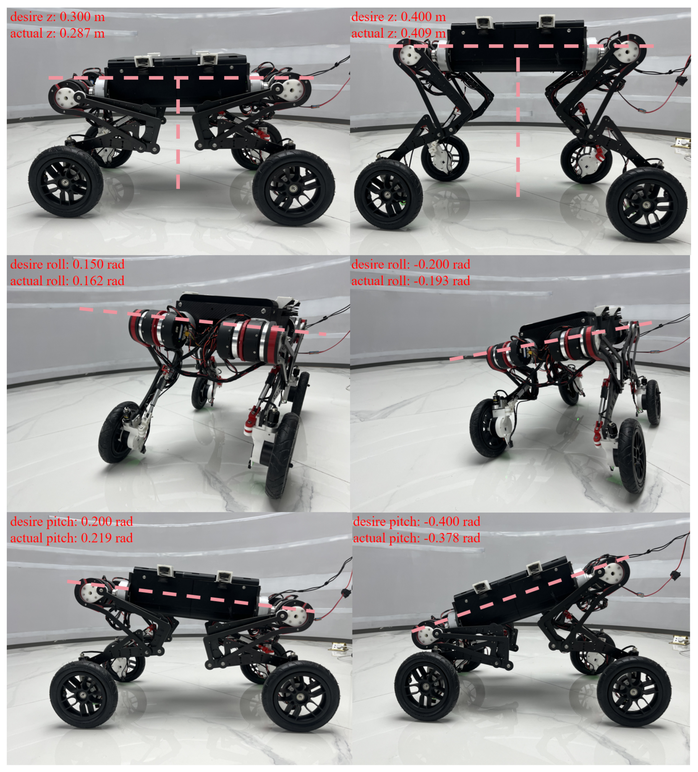
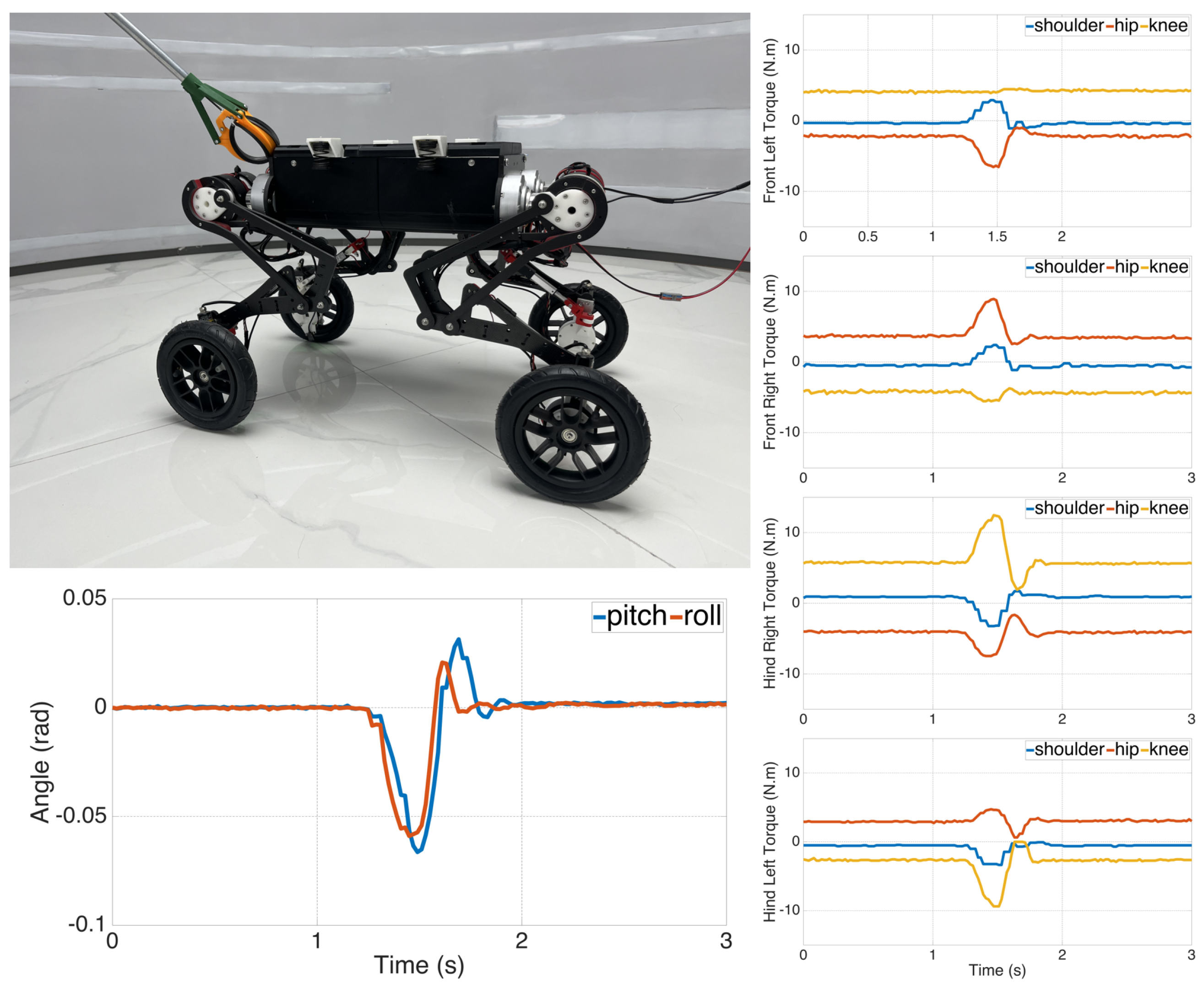
5.1.1. Posture Balancing

The initial experiments were conducted using agents trained in the pose environment. We assigned various target body posture commands and allowed Pegasus to revert to the desired state. The main desired state, the actual state of the robot, and the posture tracking performance are displayed in Figure 7. The posture error ranged between $\pm 5\%$ throughout the tests. We then introduced external disturbances to assess the robustness of agents trained under this policy. The external force applied resulted in a roll change of −0.06 radians and a pitch change of −0.07 radians. Though the body exhibited slight jitters during the process of regaining balance, the body’s balance was restored in approximately 0.8 seconds. The feedback aggregated data for 10 such experiments from the IMU and the torque are plotted in Figure 8.

5.1.2. Gait Test

In this experiment, we demonstrate the performance of the gait models (walking and trotting) we trained for Pegasus. For walking, we set the robot’s linear velocity range from 5 cm/s to 20 cm/s at 5 cm/s intervals and angular velocity from 0.05 rad/s to 0.25 rad/s at 0.05 rad/s intervals. As the robot can move faster in the trot gait, the linear velocity ranged from 5 cm/s to 30 cm/s, and angular velocity ranged from 0.05 rad/s to 0.45 rad/s at the same interval as the walk gait. To test their effectiveness, we set the target linear and angular velocities for both gaits and collected data 10 times for each sampling point. The experiments were performed on a flat terrain and traversed a distance of 15 m. The robot did not lose balance during the experiments. The results are presented in Figure 9. The graphic shows that the control deviation increases as Pegasus approaches the limit speed. For the walk gait, the maximum speed error is nearly −2 cm/s, and the maximum error of angular velocity tracking is approximately −0.05 rad/s. For the trot gait, these values are −2.5 cm/s and −0.06 rad/s, respectively.

5.1.3. Pure Driving Test

We tested agents trained MA-RL with telescopic vehicle models as motion guidance for driving mode. In this mode, we have set up a 1.5 m S-curve path for Pegasus to travel at a constant velocity of 20cm/s using its wheels and negotiate the curve using yaw. We repeated this experiment 10 times and recorded the robot’s heading and velocity. The data and images in Figure 10 demonstrate that the robot followed our preset path accurately, with a maximum deviation of only 4°. Additionally, the robot’s velocity was stable and controllable during the test runs.

6. Discussion

Real-world experiments successfully transferred trained policies to the physical Pegasus robot. The posture balancing task, for example, showed that agents trained with motion guidance could maintain desired postures effectively, recovering from external disturbances quickly despite minor jitters due to sensor noise and latency. This outcome suggests that sensor delays and environmental noise were accounted for in simulation and further tuning with hardware-in-loop. In the driving tests, Pegasus maintained heading accuracy along an S-curve path with minimal deviation, confirming the stability and adaptability of the MA-RL policies when operating on a flat surface. Gait tests for walk and trot demonstrated that the proposed framework models tracked commands near the robot’s operational limits. Tracking errors were minimal but tended to increase with the speed boundary values. This performance aligns with simulation outcomes, affirming that the trained policies can generalize well to real-world gait control tasks. For the trot gait, our proposed framework experienced slower convergence than walking as this gait requires agents to learn posture balance when two diagonal legs are scheduled simultaneously. For MA-RL and SA-RL models without motion guidance, we observed difficulty dealing with the roll and yaw of the wheeled end effectors of the Pegasus, and they converged to sub-optimal policies. In the case of SA-RL training, a spike in reward was observed before convergence, which requires further investigation.

MA-RL algorithms inherently suffer from non-stationary learning, policy convergence issues, reward shaping, and scaling [51,52]. In this paper, we have addressed these issues (apart from scaling, as the number of agents is constant) for a complex configuration of the Pegasus and successfully transferred it to the actual hardware, whereas most of the previous published work on MA-RL robotics were either based on simulation [39,53] or demonstrated in fixed-base robot with limited DoFs [54] or that tried to solve a high-level task using robots as agents [55,56,57]. A comparison with our proposed framework is not easily attainable because of the literature’s varied tasks and robot configurations. This proposed framework demonstrated promising performance, as evident in Figure 11. Compared to MA-RL (Figure 11a) and SA-RL (Figure 11a), our framework took, on average, $94.8\%$ ($26.5\times {10}^3$ epochs) and $51.7\%$ ($11.25\times {10}^3$ epochs) fewer epochs for convergence with $60\%$ (reward 85) more rewards on average across all trained tasks. However, we would like to include some observations. The current motion guidance is purely kinematic, and agents learn base and corresponding leg dynamics. We opted for kinematic motion guidance for fast optimization, and it can be reused for different robot configurations with minimal effort. The authors believe that incorporating the single rigid body kino-dynamic model used in [3,30] in motion guidance will reduce an agent’s task. Even though motion guidance took care of the individual agent’s reward and observation, another challenge for this proposed MA-RL framework is the nature of reward weight matrix tuning, which needed to be more intuitive and empirical. This issue leads directly to the next issue of the ease of implementing this framework for different robot configurations. In the future, we would like to explore multi-agent consensus and control algorithms to address these last two issues. Lastly, we used Matlab system identification and hardware-in-loop training to model the actuator; this framework will benefit simpler high-fidelity actuator models for training.

7. Conclusions

This paper presents the innovative design and development of Pegasus, a bionic wheel-legged quadruped robot with a unique chassis that enables four-wheel independent steering and diverse gaits. The main contribution is implementing an MA-RL controller for a robot with expert feedback and guidance input for multi-agent policy learning. Introducing motion guidance into the training process significantly improves the training effect; as an agent in the framework, the legs can cooperate and learn to control the floating base dynamics of the robot torso through reward function engineering. The framework addresses Pegasus’s dynamics and control strategies in a static pose, walking, trotting, and driving modes.

This MA-RL framework was designed as a proof of concept, and we did not fully explore the capabilities of Pegasus. We will add more sensors and onboard processing power to realize the robot’s dynamics and framework’s potential fully. In future research, we plan to explore communication between leg agents, introduce a parameter to modulate the states of other agents and investigate the feasibility of training a single policy for diverse terrain conditions. Additionally, we are considering implementing a switching method to dynamically select appropriate gait policies, which could lead to more adaptive and intelligent robotic locomotion in real-world scenarios.

References

1. Vukobratović, M.; Borovac, B. Zero-moment point—Thirty five years of its life. Int. J. Humanoid Robot. 2004, 1, 157–173. [Google Scholar] [CrossRef]
2. Kalakrishnan, M.; Buchli, J.; Pastor, P.; Mistry, M.; Schaal, S. Fast, robust quadruped locomotion over challenging terrain. In Proceedings of the 2010 IEEE International Conference on Robotics and Automation, Anchorage, AK, USA, 3–7 May 2010. [Google Scholar] [CrossRef]
3. Winkler, A.W.; Bellicoso, C.D.; Hutter, M.; Buchli, J. Gait and Trajectory Optimization for Legged Systems Through Phase-Based End-Effector Parameterization. IEEE Robot. Autom. Lett. 2018, 3, 1560–1567. [Google Scholar] [CrossRef]
4. Jenelten, F.; Miki, T.; Vijayan, A.E.; Bjelonic, M.; Hutter, M. Perceptive Locomotion in Rough Terrain—Online Foothold Optimization. IEEE Robot. Autom. Lett. 2020, 5, 5370–5376. [Google Scholar] [CrossRef]
5. Kim, D.; Carlo, J.D.; Katz, B.; Bledt, G.; Kim, S. Highly Dynamic Quadruped Locomotion via Whole-Body Impulse Control and Model Predictive Control. arXiv 2019, arXiv:1909.06586. [Google Scholar] [CrossRef]
6. Bjelonic, M.; Sankar, P.K.; Bellicoso, C.D.; Vallery, H.; Hutter, M. Rolling in the Deep–Hybrid Locomotion for Wheeled-Legged Robots Using Online Trajectory Optimization. IEEE Robot. Autom. Lett. 2020, 5, 3626–3633. [Google Scholar] [CrossRef]
7. Bjelonic, M.; Grandia, R.; Harley, O.; Galliard, C.; Zimmermann, S.; Hutter, M. Whole-Body MPC and Online Gait Sequence Generation for Wheeled-Legged Robots. In Proceedings of the 2021 IEEE/RSJ International Conference on Intelligent Robots and Systems (IROS), Prague, Czech Republic, 27 September–1 October 2021. [Google Scholar] [CrossRef]
8. Tan, J.; Zhang, T.; Coumans, E.; Iscen, A.; Bai, Y.; Hafner, D.; Bohez, S.; Vanhoucke, V. Sim-to-Real: Learning Agile Locomotion For Quadruped Robots. arXiv 2018, arXiv:1804.10332. [Google Scholar] [CrossRef]
9. Lyu, S.; Lang, X.; Zhao, H.; Zhang, H.; Ding, P.; Wang, D. RL2AC: Reinforcement Learning-based Rapid Online Adaptive Control for Legged Robot Robust Locomotion. In Proceedings of the Robotics: Science and Systems 2024, Delft, The Netherlands, 15–19 July 2024. [Google Scholar] [CrossRef]
10. Horak, P.; Trinkle, J.J. On the Similarities and Differences Among Contact Models in Robot Simulation. IEEE Robot. Autom. Lett. 2019, 4, 493–499. [Google Scholar] [CrossRef]
11. Lee, J.; Hwangbo, J.; Wellhausen, L.; Koltun, V.; Hutter, M. Learning Quadrupedal Locomotion over Challenging Terrain. Sci. Robot. 2020, 5, eabc5986. [Google Scholar] [CrossRef] [PubMed]
12. Kulkarni, P.; Kober, J.; Babuška, R.; Della Santina, C. Learning Assembly Tasks in a Few Minutes by Combining Impedance Control and Residual Recurrent Reinforcement Learning. Adv. Intell. Syst. 2022, 4, 2100095. [Google Scholar] [CrossRef]
13. Tao, C.; Li, M.; Cao, F.; Gao, Z.; Zhang, Z. A Multiobjective Collaborative Deep Reinforcement Learning Algorithm for Jumping Optimization of Bipedal Robot. Adv. Intell. Syst. 2023, 6, 2300352. [Google Scholar] [CrossRef]
14. Hwangbo, J.; Lee, J.; Dosovitskiy, A.; Bellicoso, D.; Tsounis, V.; Koltun, V.; Hutter, M. Learning agile and dynamic motor skills for legged robots. Sci. Robot. 2019, 4, eaau5872. [Google Scholar] [CrossRef] [PubMed]
15. Rudin, N.; Hoeller, D.; Reist, P.; Hutter, M. Learning to Walk in Minutes Using Massively Parallel Deep Reinforcement Learning. In Proceedings of the 5th Conference on Robot Learning, London, UK, 8–11 November 2021. [Google Scholar]
16. Margolis, G.; Agrawal, P. Walk These Ways: Tuning Robot Control for Generalization with Multiplicity of Behavior. In Proceedings of the 6th Conference on Robot Learning, Auckland, New Zealand, 14–18 December 2022. [Google Scholar]
17. Jenelten, F.; He, J.; Farshidian, F.; Hutter, M. DTC: Deep Tracking Control. Sci. Robot. 2024, 9, eadh5401. [Google Scholar] [CrossRef] [PubMed]
18. Melon, O.; Geisert, M.; Surovik, D.; Havoutis, I.; Fallon, M.F. Reliable Trajectories for Dynamic Quadrupeds using Analytical Costs and Learned Initializations. In Proceedings of the 2020 IEEE International Conference on Robotics and Automation (ICRA), Paris, France, 31 May–31 August 2020. [Google Scholar]
19. Surovik, D.; Melon, O.; Geisert, M.; Fallon, M.; Havoutis, I. Learning an Expert Skill-Space for Replanning Dynamic Quadruped Locomotion over Obstacles. In Proceedings of the 2020 Conference on Robot Learning, Virtual, 16–18 November 2020; Kober, J., Ramos, F., Tomlin, C., Eds.; PMLR: Proceedings of Machine Learning Research. Volume 155, pp. 1509–1518. [Google Scholar]
20. Melon, O.; Orsolino, R.; Surovik, D.; Geisert, M.; Havoutis, I.; Fallon, M.F. Receding-Horizon Perceptive Trajectory Optimization for Dynamic Legged Locomotion with Learned Initialization. In Proceedings of the 2021 IEEE International Conference on Robotics and Automation (ICRA), Xi’an, China, 30 May–5 June 2021. [Google Scholar]
21. Brakel, P.; Bohez, S.; Hasenclever, L.; Heess, N.; Bousmalis, K. Learning Coordinated Terrain-Adaptive Locomotion by Imitating a Centroidal Dynamics Planner. In Proceedings of the 2022 IEEE/RSJ International Conference on Intelligent Robots and Systems (IROS), Kyoto, Japan, 23–27 October 2022. [Google Scholar]
22. Bogdanovic, M.; Khadiv, M.; Righetti, L. Model-free Reinforcement Learning for Robust Locomotion Using Trajectory Optimization for Exploration. arXiv 2021, arXiv:2107.06629. [Google Scholar] [CrossRef]
23. Gangapurwala, S.; Geisert, M.; Orsolino, R.; Fallon, M.F.; Havoutis, I. RLOC: Terrain-Aware Legged Locomotion using Reinforcement Learning and Optimal Control. IEEE Trans. Robot. 2022, 38, 2908–2927. [Google Scholar] [CrossRef]
24. Tsounis, V.; Alge, M.; Lee, J.; Farshidian, F.; Hutter, M. DeepGait: Planning and Control of Quadrupedal Gaits using Deep Reinforcement Learning. IEEE Robot. Autom. Lett. 2020, 5, 3699–3706. [Google Scholar] [CrossRef]
25. Xie, Z.; Da, X.; Babich, B.; Garg, A.; van de Panne, M. GLiDE: Generalizable Quadrupedal Locomotion in Diverse Environments with a Centroidal Model. In Proceedings of the Fifteenth Workshop on the Algorithmic Foundations of Robotics, College Park, MD, USA, 22–24 June 2022. [Google Scholar]
26. Wu, J.; Xin, G.; Qi, C.; Xue, Y. Learning Robust and Agile Legged Locomotion Using Adversarial Motion Priors. IEEE Robot. Autom. Lett. 2023, 8, 4975–4982. [Google Scholar] [CrossRef]
27. Cui, L.; Wang, S.; Zhang, J.; Zhang, D.; Lai, J.; Zheng, Y.; Zhang, Z.; Jiang, Z.P. Learning-Based Balance Control of Wheel-Legged Robots. IEEE Robot. Autom. Lett. 2021, 6, 7667–7674. [Google Scholar] [CrossRef]
28. Lee, J.; Bjelonic, M.; Hutter, M. Control of Wheeled-Legged Quadrupeds Using Deep Reinforcement Learning. In Robotics in Natural Settings, Proceedings of the Climbing and Walking Robots Conference, Ponta Delgada, Portugal, 12–14 September 2022; Springer: Cham, Switzerland, 2022; pp. 119–127. [Google Scholar]
29. Pan, Y.; Khan, R.A.I.; Zhang, C.; Zhang, A.; Shang, H. Pegasus: A Novel Bio-inspired Quadruped Robot with Underactuated Wheeled-Legged Mechanism. In Proceedings of the 2024 IEEE International Conference on Robotics and Automation (ICRA), Yokohama, Japan, 13–17 May 2024; pp. 1464–1469. [Google Scholar] [CrossRef]
30. Rezwan Al Islam, K.; Chenyun, Z.; Yuzhen, P.; Anzheng, Z.; Ruijiao, L.; Xuan, Z.; Huiliang, S. Hierarchical optimum control of a novel wheel-legged quadruped. Robot. Auton. Syst. 2024, 180, 104775. [Google Scholar] [CrossRef]
31. Littman, M.L. Markov games as a framework for multi-agent reinforcement learning. In Proceedings of the Eleventh International Conference on International Conference on Machine Learning, ICML’94, New Brunswick, NJ, USA, 10–13 July 1994; pp. 157–163. [Google Scholar]
32. Watkins, C.J.C.H. Learning from Delayed Rewards. Ph.D. Thesis, King’s College, Oxford, UK, 1989. [Google Scholar]
33. Mnih, V.; Kavukcuoglu, K.; Silver, D.; Rusu, A.A.; Veness, J.; Bellemare, M.G.; Graves, A.; Riedmiller, M.; Fidjeland, A.K.; Ostrovski, G.; et al. Human-level control through deep reinforcement learning. Nature 2015, 518, 529–533. [Google Scholar] [CrossRef]
34. Hasselt, H. Double Q-learning. In Proceedings of the Advances in Neural Information Processing Systems 23: 24th Annual Conference on Neural Information Processing Systems 2010, Vancouver, BC, Canada, 6–9 December 2010; Volume 23. [Google Scholar]
35. Sutton, R.S.; McAllester, D.; Singh, S.; Mansour, Y. Policy Gradient Methods for Reinforcement Learning with Function Approximation. In Proceedings of the Advances in Neural Information Processing Systems 12, NIPS Conference, Denver, CO, USA, 29 November–4 December 1999; Volume 12. [Google Scholar]
36. Lillicrap, T.P.; Hunt, J.J.; Pritzel, A.; Heess, N.; Erez, T.; Tassa, Y.; Silver, D.; Wierstra, D. Continuous control with deep reinforcement learning. In Proceedings of the 4th International Conference on Learning Representations, ICLR 2016, San Juan, Puerto Rico, 2–4 May 2016. Conference Track Proceedings. [Google Scholar]
37. Fujimoto, S.; van Hoof, H.; Meger, D. Addressing Function Approximation Error in Actor-Critic Methods. In Proceedings of the 35th International Conference on Machine Learning, ICML 2018, Stockholmsmässan, Stockholm, Sweden, 10–15 July 2018; Dy, J.G., Krause, A., Eds.; PMLR: Proceedings of Machine Learning Research. Volume 80, pp. 1582–1591. [Google Scholar]
38. Lowe, R.; Wu, Y.; Tamar, A.; Harb, J.; Abbeel, P.; Mordatch, I. Multi-agent actor-critic for mixed cooperative-competitive environments. In Proceedings of the 31st International Conference on Neural Information Processing Systems, NIPS’17, Long Beach, CA, USA, 4–9 December 2017; pp. 6382–6393. [Google Scholar]
39. Ackermann, J.; Gabler, V.; Osa, T.; Sugiyama, M. Reducing Overestimation Bias in Multi-Agent Domains Using Double Centralized Critics. arXiv 2019, arXiv:1910.01465. [Google Scholar] [CrossRef]
40. Zhang, F.; Li, J.; Li, Z. A TD3-based multi-agent deep reinforcement learning method in mixed cooperation-competition environment. Neurocomputing 2020, 411, 206–215. [Google Scholar] [CrossRef]
41. Pomax. A Primer on Bézier Curves. 2021–2024. Available online: https://pomax.github.io/bezierinfo/ (accessed on 22 November 2024).
42. Miki, T.; Lee, J.; Hwangbo, J.; Wellhausen, L.; Koltun, V.; Hutter, M. Learning robust perceptive locomotion for quadrupedal robots in the wild. Sci. Robot. 2022, 7, eabk2822. [Google Scholar] [CrossRef] [PubMed]
43. Coumans, E.; Bai, Y. PyBullet, a Python Module for Physics Simulation for Games, Robotics and Machine Learning. 2016–2021. Available online: http://pybullet.org (accessed on 25 October 2024).
44. MathWorks. Identifying State-Space Models with Separate Process and Measurement Noise Descriptions. 2024. Available online: https://www.mathworks.com/help/ident/ug/identifying-state-space-models-with-independent-process-and-measurement-noise.html (accessed on 22 November 2024).
45. Nvidia. Jetson Orin. 2024. Available online: https://www.nvidia.com/en-us/autonomous-machines/embedded-systems/jetson-orin/ (accessed on 25 October 2024).
46. Unitree a1 Motor. Available online: https://shop.unitree.com/products/unitree-a1-motor (accessed on 25 February 2024).
47. LK MG6010 Geared Motor. Available online: http://shop.smc-powers.com/MG6010-CAN-D.html (accessed on 25 February 2024).
48. STM32F446 Resource. Available online: https://www.st.com/en/microcontrollers-microprocessors/stm32f446.html (accessed on 25 February 2024).
49. Saber C4 Resource. Available online: http://www.atom-robotics.com/PC-EN/productC4.html (accessed on 25 February 2024).
50. BRT25 Product Catalog. Available online: https://briterencoder.com/wp-content/uploads/2021/12/BriterEncoder-Product-Catalogue-V2.3.pdf (accessed on 25 February 2024).
51. Busoniu, L.; Babuska, R.; Schutter, B.D. Multi-Agent Reinforcement Learning: An Overview; Technical Report; Delft University of Technology: Delft, The Netherlands, 2010. [Google Scholar]
52. Albrecht, S.V.; Christianos, F.; Schäfer, L. Multi-Agent Reinforcement Learning: Foundations and Modern Approaches; MIT Press: Cambridge, MA, USA, 2024. [Google Scholar]
53. Sebastian, E.; Duong, T.; Atanasov, N.; Montijano, E.; Sagues, C. Physics-Informed Multi-Agent Reinforcement Learning for Distributed Multi-Robot Problems. arXiv 2024, arXiv:2401.00212. [Google Scholar] [CrossRef]
54. Perrusquía, A.; Yu, W.; Li, X. Redundant Robot Control Using Multi Agent Reinforcement Learning. In Proceedings of the 2020 IEEE 16th International Conference on Automation Science and Engineering (CASE), Hong Kong, China, 20–21 August 2020; pp. 1650–1655. [Google Scholar] [CrossRef]
55. Brandão, B.; De Lima, T.W.; Soares, A.; Melo, L.; Maximo, M.R.O.A. Multiagent Reinforcement Learning for Strategic Decision Making and Control in Robotic Soccer Through Self-Play. IEEE Access 2022, 10, 72628–72642. [Google Scholar] [CrossRef]
56. Orr, J.; Dutta, A. Multi-Agent Deep Reinforcement Learning for Multi-Robot Applications: A Survey. Sensors 2023, 23, 3625. [Google Scholar] [CrossRef]
57. Yu, C.; Yang, X.; Gao, J.; Chen, J.; Li, Y.; Liu, J.; Xiang, Y.; Huang, R.; Yang, H.; Wu, Y.; et al. Asynchronous Multi-Agent Reinforcement Learning for Efficient Real-Time Multi-Robot Cooperative Exploration. arXiv 2023, arXiv:2301.03398. [Google Scholar] [CrossRef]
Figure 1. The image displays frames of Pegasus. The axes are color-coded: red for the x-axis, green for the y-axis, and blue for the z-axis. On the left side, the frames of the entire body in the world frame { F W } are shown, while the right side illustrates the frames of one of the robot’s 5 DoF legs [30].
Machines 12 00902 g001
Figure 2. The contact model of the Pegasus is outlined as follows. Panel (a) presents a schematic representation of the robot’s walking gait. We detail the contact force, represented by the friction cone ( F ee i ς ( i , μ ˜ c ) ), along with the various directions of the end effector’s velocity: x , y , and z n . Panel (b) features an ellipse that represents the utility function (as detailed in Equation (13)) [30].
Machines 12 00902 g002
Figure 3. Telescopic vehicle model. Sketch of the telescopic vehicle model of Pegasus. The robot rotates counterclockwise, and the detailed parameters of the left front leg are shown. LF: left front; RF: right front; LH: left hind; RH: right hind.
Machines 12 00902 g003
Figure 4. Overview of the training flow and deployment strategy.
Machines 12 00902 g004
Figure 5. Gym-like environment. Illustration of the gym environment generated from 8-bit grayscale images. The right side shows grayscale image input, and the left side shows the resulting environment.
Machines 12 00902 g005
Figure 6. Reward comparison. Four models were trained for each motion mode (a) Static Pose, (b) Walk, (c) Static Pose and (d) Walk. The lines in every figure depict the mean value of the four agents’ rewards: the red line depicts the reward MA-RL without motion guidance, the yellow line depicts the reward SA-RL without motion guidance, and the blue line depicts the reward with motion guidance. We can see that the agents can attain a higher reward and faster convergence speed with the motion guidance.
Machines 12 00902 g006
Figure 7. Based on the proposed method, the robot is capable of highly flexible movement. The accompanying figure demonstrates the robot’s ability to adjust its height and orientation angle in response to specific instructions.
Machines 12 00902 g007
Figure 8. The pictures illustrate the application of external disturbances and how they affect the robot’s balance and torque measurements.
Machines 12 00902 g008
Figure 9. Gait test. The pictures are actual pictures taken during the experiment. Red circles highlight a leg in swing state and orange ground symbols show a leg in stance. The data shows the velocity and angular velocity tracking errors of the robot. Each point with an error bar shown in the following data is the mean value of the 10 samples we collected.
Machines 12 00902 g009
Figure 10. Pure driving test. The first few real shots record the overall trajectory we preset and the actual pictures while Pegasus is passing by. The data shows the actual and desired heading angle and velocity(the velocity is set as 20 cm/s) of Pegasus during the experiment.
Machines 12 00902 g010
Figure 11. Illustrations of our proposed framework’s convergence and reward percentage difference vs. (a) MA-RL (without guidance) and (b) SA-RL (without guidance) for four trained models. The arrows’ direction indicates if a particular parameter is increasing or decreasing compared to our framework.
Machines 12 00902 g011