1. Introduction
Solar arrays, or Photovoltaic (PV) grids, are essential for sustainable energy production, addressing environmental and economic concerns [
1]. They harness sunlight to generate electricity, providing a renewable and clean energy source that reduces reliance on fossil fuels and minimizes greenhouse gas emissions [
2]. Solar arrays contribute to energy security by diversifying the energy supply, and they can be deployed at various scales, from residential rooftops to large solar farms. Additionally, they promote energy independence and have the potential to reduce electricity costs over time significantly [
3]. Their implementation supports the global shift to a low-carbon economy and helps alleviate the impacts of climate change [
4]. However, issues with solar arrays or PV grids can significantly impact their efficiency, safety, and overall performance. Common problems include the following: shading, which can reduce the output of individual panels and the entire system; micro-cracks or hotspots, which can degrade panels over time; and connection problems, such as loose or corroded wiring, which can disrupt the flow of electricity [
5]. Inverter faults, which convert the direct current (DC) output of solar panels to alternating current (AC) for grid use, can also lead to substantial energy losses [
6]. Thus, monitoring and diagnostic systems are crucial for the early detection and resolution of these faults to maintain optimal operation and extend the lifespan of solar installations. Regular maintenance and inspection are also essential to ensure reliability, prevent potential hazards, and maximize energy production from PV grids.
There are two different methods for detecting faults within a Solar or PV system. These are first-principal or model-driven and data-driven methods [
7,
8]. The former involves the establishment of a physical model or mathematical model, while the latter relies on control system’s sensor/IoT data [
8]. Data-driven models can be implemented using either shallow learning techniques or deep learning (DL) techniques, both of which provide reliable and efficient solutions for fault detection when compared to model-driven approaches [
9,
10]. DL is particularly effective at analyzing complex supervisory control and data acquisition (SCADA) data. Within the scope of DL, there are two primary approaches to fault detection: forecasting-based techniques and reconstruction-based techniques [
11]. This paper, however, exclusively centers on reconstruction-based techniques, providing a detailed and comprehensive understanding of this specific approach.
Models based on an autoencoder (AE) [
12,
13,
14], including long short-term memory (LSTM) and convolutional neural network (CNN) models, as well as variational, sparse, and denoising types, are commonly used models for fault detection in different applications [
15,
16]. For example, stacked AE-based models are used for solar array fault diagnosis in [
17,
18]. However, the stacked AE-based models have multiple hidden layers, which can lead to overfitting. Seghiour et al. [
19] combined an AE and a feed-forward neural network to diagnose and classify faults in solar PV arrays. Ayobami et al. [
20] proposed Variational AE (VAE) and spread spectrum techniques to detect, isolate, and characterize faults in PV systems. LSTM AE-based models with wavelet packet-transformed PV signals are proposed in [
21,
22]. Similarly, AE and its variants are applied to fault diagnosis for solar arrays in [
23,
24,
25]. However, the AE-based models often struggle to capture SCADA data’s spatial and temporal relationships [
26,
27].
To gain comprehensive insights, it is essential to consider these relationships together [
27]. Graph neural networks (GNNs) excel at learning spatiotemporal data due to their unique features, such as permutation invariance and local connectivity [
11]. Researchers have employed GNNs, particularly graph convolutional networks (GCNs), to develop spatiotemporal autoencoders for fault identification, achieving better results than traditional AEs across various process monitoring applications [
26,
28,
29,
30,
31]. However, GCN-enabled VAE is not adequately investigated for fault diagnosis in industrial applications. VAE offer several advantages over conventional AE models. For example, VAE incorporate a regularization term (the Kullback–Leibler divergence) in their loss function, encouraging the latent space to conform to a standard normal distribution [
32,
33]. This helps prevent overfitting and ensures a more uniform latent space [
32]. The latent representations learned through VAE are often more informative and disentangled than those obtained via traditional AE. This can improve performance in downstream tasks such as clustering, classification, or anomaly detection.
This study uses the GCN model to develop a VAE to detect faults in PV microgrids within renewable energy applications. The GCN’s capacity to learn spatiotemporal features renders it exceptionally well suited for SCADA data’s intricate nonlinear spatiotemporal modeling. Moreover, skip connections are added between the models hidden layers to mitigate the loss of information for the encoding–decoding process.
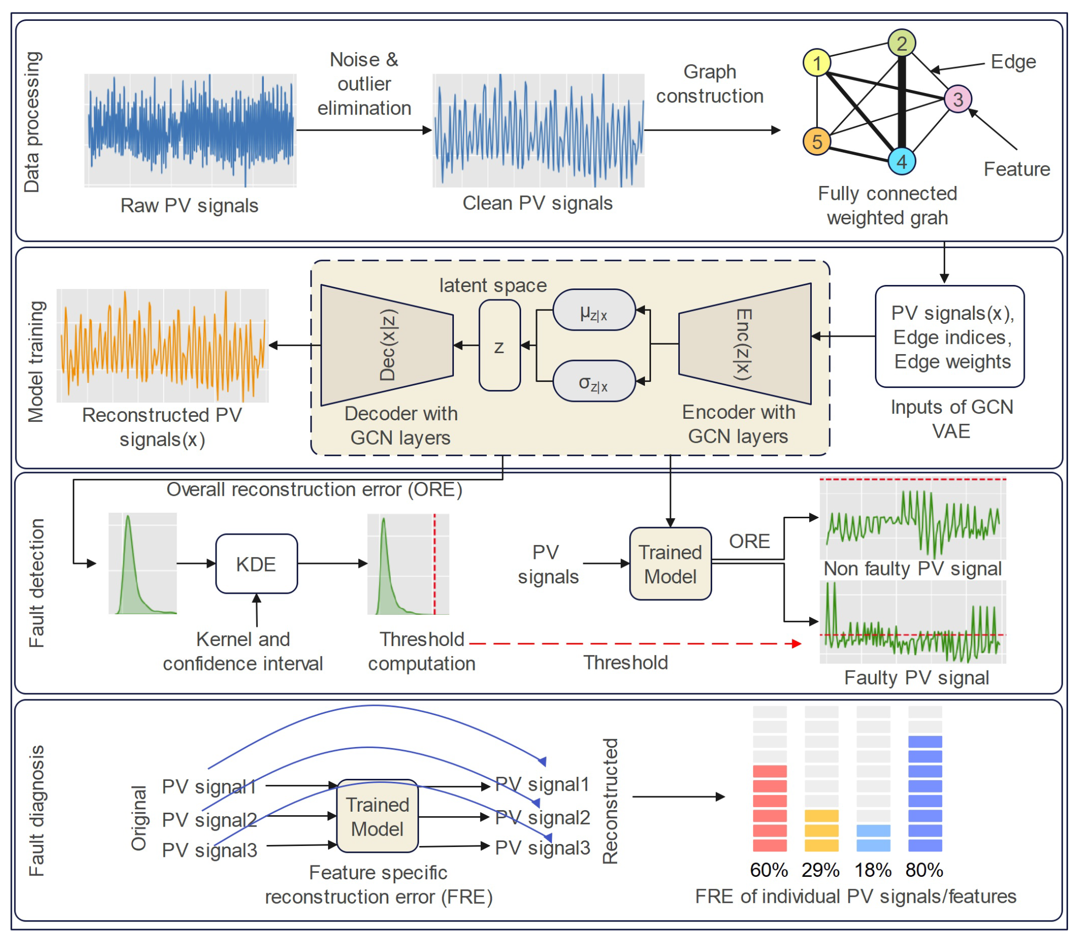
Figure 1 shows the proposed fault detection and diagnosis framework for the GCN-based VAE model. The major contributions of this paper are outlined as follows.
A VAE model based on GCN layers is developed to detect faults in solar array applications. The GCN VAE model effectively learns the spatiotemporal characteristics of SCADA sensor data, outperforming conventional AE models.
We use the convolutional filter and boxplot algorithm to enhance the data quality. The convolutional filter reduces noise, while the boxplot removes outliers from the noisy sensor data.
The performance of the GCN-VAE model is evaluated based on a solar array dataset and compared with the conventional AE models
The false alarm rate (FAR) and fault detection rate (FDR) show that the proposed GCN-based VAE outperforms conventional AE models.
Also, individual feature reconstruction errors are analyzed for diagnosing the root cause of a fault.
Section 2 explains the fault detection and diagnosis process using the GCN-based VAE model. We first provide a brief overview of the GCN and then demonstrate how it is integrated with the VAE to create a DL model for fault detection. Finally, we discuss the fault detection indicators and the diagnosis process.
Section 3 presents the experimental procedure, including data processing, model training, testing, and results. Finally,
Section 4 concludes the paper.
2. GCN VAE-Based Fault Detection and Diagnosis
This section discusses GCN and GCN-based VAE for detecting faults in PV or solar array systems. Then, it is shown how the reconstruction error of the GCN VAE can be used to identify faulty components (features) within the larger system.
2.1. Graph Convolutional Network
We can define a graph as
, which contains a set of nodes,
V,
, a set of edges,
E,
, and an adjacency matrix,
A. The graph’s adjacency matrix,
, expresses the relationships of weights and edges among the graph nodes,
V. Therefore, if we find an edge between node
and
, then these two nodes are neighbors
, and the corresponding entry,
in
A, refers to the weights of the edge. We can use various techniques, such as Euclidean similarity, a correlation matrix, or cosine similarity, to compute the weights of the edges [
13]. On the other hand, the entries of the adjacency matrix,
A, of an unweighted graph can be set to
.
Graph convolution networks use spectral and spatial approaches, with spectral methods based on graph signal processing and defining the convolution operator in the spectral domain. Spectral methods involve transforming a graph signal,
x, using the graph Fourier transform,
, conducting a convolution operation, and then transforming back the resulting signal using the inverse graph Fourier transform
[
34,
35]. Mathematically,
where
U is the normalized graph laplacian matrix
;
D,
A are the degree and adjacency matrix, respectively. Then, according to the convolution operation,
where
is the spectral domain filter. The principal function of the spectral method can be defined by simplifying the filter through a learnable diagonal matrix
. Defferrard et al. [
36] approximated the
in their proposed Chebynet model with Chebyshev polynomials
up to
order. The ChebNet model operation can be described as
where
is the largest eigenvalue of
L. However, in this work, GCN proposed by Kipf [
37] is used in constructing the AE model. Kipf simplified the convolution operation of ChebNet by setting
and
to overcome the overfitting problem. Using these assumptions, the operation of GCN can be defined as
Kipf further introduced the renormalization trick to overcome the exploding/vanishing gradient problem by updating
and
. Finally, the convolution operation of GCN can be defined as
where
X is the input data matrix,
W is the model parameters, and
H is the resulting convolution matrix. The GCN based on the spectral method is used in this paper to construct the fault diagnosis model.
2.2. Graph Convolutional Network-Based Variational Autoencoder
This work develops a graph convolutional variational autoencoder (GCVAE) model that combines GCN and VAE to learn spatiotemporal time series data representations. First, the time series data are represented as a graph by defining nodes, computing edges, and edge weights. Then, the GCN-based variational encoder is used to encode the graph-structured spatiotemporal time series data. Each feature in the time series data is considered a node (
V) in the graph, and a fully connected weighted graph (
) is assumed, meaning that each feature (
V) is connected to all the other features. The edge weights (
) are calculated based on the cosine similarity metric. The model consists of a multi-layer GCN-based variational encoder and decoder architecture. The encoder
generates the latent representation of the time series data by taking into account the edges (
) and edge weights (
). On the other hand, the decoder
generates reconstructed data
based on the latent representation
z along with the edges (
), and the edge weights (
). The output of the
encoder layer can be written as a function of the previous layer output and the adjacency matrix A, the edge indices (
), and the edge weights (
) as
where
,
, and
are the activation function, weight matrix, and the encoded representation of layer
l. On the contrary, the
layer of the decoder can be mathematically represented as
Similarly to the VAE, the GCVAE also optimizes the encoder and decoder parameters
and
by minimizing the below loss function through the backpropagation algorithm.
Since the GCN model is capable of learning the spatiotemporal relation among the features, the GCN-based VAE can learn the spatiotemporal data more effectively than other conventional AE models.
2.3. Graph-Convolutional Variational Autoencoder for Fault Detection
Microgrid operation produces significant data, which SCADA systems gather and store. Nevertheless, most of these data arise from normal operational circumstances, and faulty data are infrequent and occasionally inaccessible. This section endeavors to develop a standard reference model utilizing this normal data (fault-free data). Through this reference model, testing data can be assessed to recognize and identify potential faults. Therefore, in this section, a GCN VAE-based fault detection model is presented that learns the non-linear spatiotemporal SCADA data from the normal operation of the PV panel. The model learns the latent representation of the spatiotemporal SCADA data by reconstructing it, which makes it more robust than other AE-based models.
Unlike other AE-based detection methods, a GCN VAE detection model cannot be trained directly on multivariate sensor data to comprehensively understand their intrinsic representation and the spatial and temporal connections between them. Multivariate time-series sensor data needs to be converted into graph-structure data. The previous subsection explains the process of transforming the time series data into graph-structured data. Let
be the normal multivariate SCADA data from the PV panel, where
M is the number of features (sensors), and
N is the number of data samples. The dataset
X is split into training, validation, and testing data as
. Then, for training, the graph attributes are generated from
for the adjacency matrix
A, i.e., the edges and weights of each edge. A fully connected graph is considered for this work, meaning that all the nodes are connected with each other, and finally, the model computes the edge weights using the cosine similarity metric. The cosine similarity between two nodes or features,
and
, can be defined as follows:
where
, and
After the graph attributes are generated, the GCN VAE model is trained by passing the data,
, and the adjacency matrix,
A, to minimize the loss function defined in Equation (
8) for learning the optimal encoder and decoder parameters. Only the normal train data split,
, is used to train the model. Upon the completion of training, the model excels in precisely reconstructing normal data, while faulty samples from the faulty data,
, produce noticeable spikes in reconstruction error. Therefore, a reconstruction error-based fault detection indicator can detect possible faults in the testing data [
38].
2.4. Fault Detection Indicator Construction
Squared prediction error (SPE) residuals,
, are used here to represent the reconstruction error for all the samples,
. The SPE is computed on the validation data,
, to determine the fault indicator threshold as follows:
Then, the threshold or control limit of
is computed using the statistical properties of its distributions. However, in this case, the distribution is unknown in advance; therefore, it is needed to estimate the probability density functions of
E through a non-parametric kernel density estimation (KDE) technique. KDE is a widely accepted and proven methodology for estimating the probability density function (PDF), and it has demonstrated remarkable success in process monitoring and fault detection. We used the KDE method to compute the threshold. The estimated PDF of error points, say
,
at point
r, can be mathematically defined as [
13]
where
is the kernel function, and
is the bandwidth. Here, the Gaussian kernel function
and the Silverman bandwidth are used. Finally, we can compute the threshold
of the error vector
E using the estimated PDF for a given confidence value,
, by solving the following equation [
38]:
In the online monitoring phase, any data sample that exceeds the threshold is classified as a faulty sample.
2.5. Fault-Diagnosis Process
Fault diagnosis is a process that helps accurately identify the root cause of problems, enabling corrective action. It is also known as “fault isolation”, which differentiates it from fault detection. In this work, diagnosis aims to identify the sensor responsible for the system failure. To achieve this, the reconstruction error is analyzed for individual features that contribute more than the others to each type of fault in the overall reconstruction error.
3. Experiments and Results
To conduct the experiment for evaluating the proposed fault detection and diagnosis model, a solar/PV array microgrid dataset from a recent article [
6] was considered. The overview of the proposed framework is presented in
Figure 1. We first de-noised and removed outliers from the raw data. Then, from the cleaned data, we generated the graph attributes and trained the model. The KDE is used to determine the threshold from the trained model’s reconstruction error. Finally, the individual reconstruction error for each feature was used to identify the faulty components in the diagnosis phase.
3.1. Dataset Explanation
In a laboratory environment, the authors of [
6] implemented a PV microgrid system to collect both normal and faulty operational data from Integrated Power Probability Table (IPPT) mode. The data encompass various sensor signals, including time, PV array current, voltage, DC voltage, three-phase current measurements, three-phase voltage measurements, current magnitude, current frequency, voltage magnitude, and voltage frequency. Deliberate faults were introduced, such as inverter faults (Fault 1), feedback sensor faults (Fault 2), grid anomalies (Fault 3), PV array mismatches (Fault 4 (10% to 20%), and Fault 5 (15%)), as well as controller faults (Fault 6) and converter faults (Fault 7).
Table 1 shows the statistical summary of the dataset.
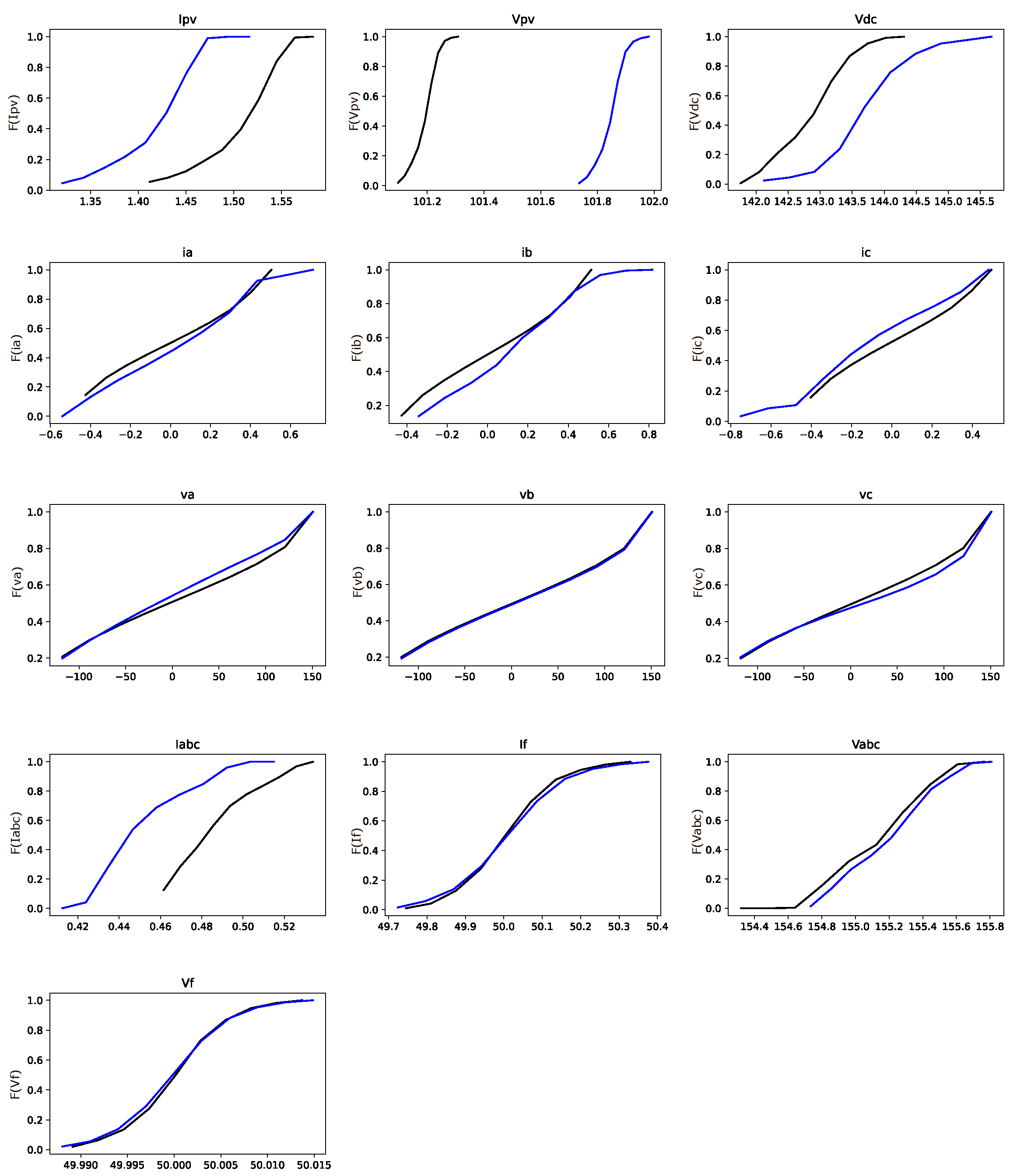
Figure 2 demonstrates the use of the Kolmogorov–Smirnov (KS) test in analyzing the IPPT dataset of fault type 1 and the standard set. The KS test is employed here to understand the statistical difference (cumulative distribution function (CDF)) between each feature from the standard and faulty part of the dataset. The KS test is a non-parametric statistical test used to compare a sample distribution with a reference probability distribution or to compare two sample distributions. It evaluates the null hypothesis that the samples are drawn from the same distribution without assuming any specific form for the distribution [
39]. The test assesses the maximum difference between the empirical distribution function of the sample and the cumulative distribution function of the reference distribution or between the empirical distribution functions of two samples. A significant KS test result indicates that the distributions differ significantly. It is a valuable tool for testing assumptions about data distributions and detecting deviations from expected patterns.
Based on the KS test, the Vpv feature displays considerably greater differences between standard and faulty parts of the dataset compared to other features.
Table 2 presents the numerical results of the KS test for all fault types. It is evident from
Table 2 that the Vpv feature is responsible for making the solar array defective across all fault types (marked as bold).
3.2. Data Preprocessing
The proposed fault detection and diagnosis framework’s data preprocessing module comprises a convolution filter-based noise-reduction method and a boxplot-based outlier-removal technique.
3.2.1. Convolution Filter-Based Noise Reduction
In this work, a convolution filter [
40,
41] is applied to reduce the effect of noise from each feature. Convolutional filter-based signal smoothing is a method that aims to reduce noise and highlight essential features within a signal. This technique works by sliding a filter (kernel) across the targeted signal and conducting element-wise multiplications and summations. The filter coefficients can be of different types, such as Gaussian or moving-average filters, which determine the extent of the smoothing effect. Convolutional filters can reduce the impact of high-frequency noise while maintaining the low-frequency components. This filtering technique has widespread usage for enhancing data quality in domains such as computer vision, signal processing, time-series sensor data analysis, etc. Therefore, it improves the interpretation and analysis of the underlying dataset. Moreover, the adaptability and efficiency of this technique have made it suitable for real-time applications with large-size datasets.
3.2.2. Boxplot for Outlier Removing
A boxplot is a straightforward and effective method for identifying and eliminating outliers from a dataset [
42]. A boxplot provides a five-number summary of a data set [
43]: the minimum value
, the maximum value
, the first quartile (
), the median value (the second quartile (
)), and the third quartile (
). This method produces the
range and the interquartile range (
); using these ranges, a boundary can be established to distinguish outliers from standard data samples. Mathematically, we can say that any data points above
and below
are outliers, and then we can remove those data points from the original data series [
13].
Therefore, the noisy components from each feature of the dataset are removed using the convolution filter algorithm with different window sizes. The resulting features were then subjected to the boxplot method to remove any outliers from training, validation, and testing data.
Figure 3 shows the effect of applying the convolutional filter and boxplot on the Ipv feature of the dataset.
3.3. Model Training and Testing
The primary step for training the proposed DL model is to normalize the dataset using Python’s StandardScaler function (
https://scikit-learn.org/stable/modules/generated/sklearn.preprocessing.StandardScaler.html accessed 21 August 2024). The StandardScaler function (
, where
is the mean and
is the standard deviation) is first applied to the training data (fault-free dataset) to normalize it; then, the mean and standard deviation of the fault-free training data is used to normalize the validation data (fault-free) and test data (faulty data). After that, the edge index and weights of the graph are generated based on the cosine similarity metric. Finally, the processed training data, its edge indices, and edge weights are transferred to the models for training. The first 7000 data points of the fault-free training data are utilized to train the model, and an additional 2000 data points of the fault-free training data are marked for validation. Subsequently, the trained model was tested using 1000 data points for each type of fault. The hyperparameters were chosen through a trial and error approach, wherein the loss function was carefully monitored to identify the parameters that yielded the lowest reconstruction error. The lowest reconstruction error was found for the Adam Optimiser, which has a learning rate of 0.001 and 3000 epochs. Also, experiments were conducted for two different window sizes of the convolutional filter and three different hidden layer dimensions.
3.4. Threshold Selection
Once the model has been trained, the validation dataset is evaluated and used to compute the SPE error [
13]. Next, the threshold is calculated from the SPE using the Gaussian KDE estimation method, following the Equation
for a confidence value of
. In the test set, any data points exceeding the threshold are classified as faulty, while those below the threshold are considered non-fault samples.
3.5. Results
The fault detection rate and false alarm rate are used to evaluate the model’s performance on fault detection and false alarm suppression. These critical metrics are instrumental in assessing the efficacy of fault detection systems. The FDR indicates the proportion of faults correctly identified through the system, thereby illustrating its ability to recognize genuine issues. A DL model with high FDR ensures the reliability, safety, and timely detection of most faults in the underlying cyber-physical systems. On the contrary, the FAR measures the percentage of non-faulty conditions inaccurately predicted as faults. These evaluation metrics reflect the DL model’s precision in differentiating the normal states from the faulty states. A high FAR can result in unwanted human interventions, increased maintenance costs, and reduced confidence in the system’s accuracy. Striking a balance between FDR and FAR is essential; an optimal fault detection system maximizes FDR while minimizing FAR, enabling efficient and dependable operation with minimal false alarms. The FDR and FAR are defined mathematically as follows [
13]
Here,
indicates the number of detected faults, while
refers to the total count of faulty samples.
Here, indicates the number of detected normal samples, while refers to the total count of normal data samples.
Table 3 outlines the FDR about different fault types for the GCN VAE when the number of nodes in the bottleneck layer (or latent dimension) is varied (for 1, 2, and 3 nodes in the bottleneck layer). This table indicates that the GCN VAE demonstrates optimal fault detection performance when two nodes/neurons are in the bottleneck layer, as evidenced by a decline in performance for Fault 3 and Fault 5 when the latent dimensions were 1 and 3. However, the model’s performance remains relatively consistent across all three bottleneck layers for other fault types. Furthermore, the table also presents the FDR after introducing skip connections between the layers of the GCN VAE. Without skip connections, the FDR decreases to 9 and 0 for Fault 3 and Fault 6, respectively, and consequently fails to detect Fault 5 correctly (32% FDR for fault type 5). Conversely, with skip connections, the model can detect all fault types with an FDR exceeding 95%.
In this work, the FDR performance of the GCN VAE is evaluated alongside other conventional autoencoder-based diagnosis models such as Feedforward AE, LSTM-AE, and LSTM VAE.
Table 4 shows this comparison results. We conducted the comparison using two different window sizes for the convolutional filter. For the convolution filter’s window size of 25, the GCN VAE achieved a similar FDR to AE, LSTM AE, and LSTM VAE for Fault 1, Fault 2, Fault 4, and Fault 7. However, the GCN VAE outperformed the other models in detecting Fault 3 and Fault 6. It is worth noting that the window size of 25 for the convolution filter couldn’t effectively eliminate noise from the signals. Consequently, none of the models, including GCN VAE, could achieve significant performance for Fault 5. In the context of a window size of 35, the GCN VAE exhibited superior overall performance compared to other baseline models. Specifically, the GCN VAE achieved a fault detection rate of over 95% across all types of faults. For Fault 1, Fault 2, Fault 3, and Fault 4, all models demonstrated similar detection performance, with the exception of the LSTM VAE, which did not perform well for Fault 3. Additionally, for Fault 5, the GCN VAE outperformed all other models with a 95% detection rate. For Fault 6 and Fault 7, again, the GCN VAE outperformed other models with 99% FDR.
Figure 4 illustrates the comparison results of
Table 3 and
Table 4 graphically.
The FAR metric is also considered to evaluate the proposed models’ performance. The GCN VAE achieved 0.3% and 0.1% false alarm rates for convolutional window sizes of 25 and 35, respectively. However, the LSTM AE showed 0.15% and 0.18%; LSTM VAE showed 0.09% and 0.07%; and finally, the feed-forward AE model gained 1.05% and 1.55% FAR for convolution window sizes 25 and 35, respectively. Although LSTM VAE showed good FAR compared to the GCN VAE, still, the FAR for GCN VAE is less than 1%.
We validated the model’s capability to identify the faulty sensor or feature-causing system malfunctions. In order to do so, we intentionally introduced noise to each feature individually while keeping the others unchanged. Subsequently, we computed the reconstruction error for each feature. The results are displayed in
Table 5, showing the reconstruction error for each feature of the GCN VAE with a noise mean of 1.50 and a standard deviation of 3.50. The initial row of the table displays the reconstruction errors for each feature in the absence of added noise. The table clearly indicates that modifying the Ipv feature leads to a higher reconstruction error compared to the other features, which remain unchanged. This pattern also holds when noisy components are added to other features. Furthermore, the reconstruction error of the noisy features is notably higher than that of the features without noise. Similarly,
Table 6 shows the effect of individual reconstruction error of the features with and without noise for a noise mean of 2.50 and a standard deviation of 4.50. From these tables, we can observe that the reconstruction errors for the features are increased from
Table 5 to
Table 6 with the increase in noise density.
Based on our validation process, we can confidently utilize the GCN VAE model to detect faulty components in the PV array.
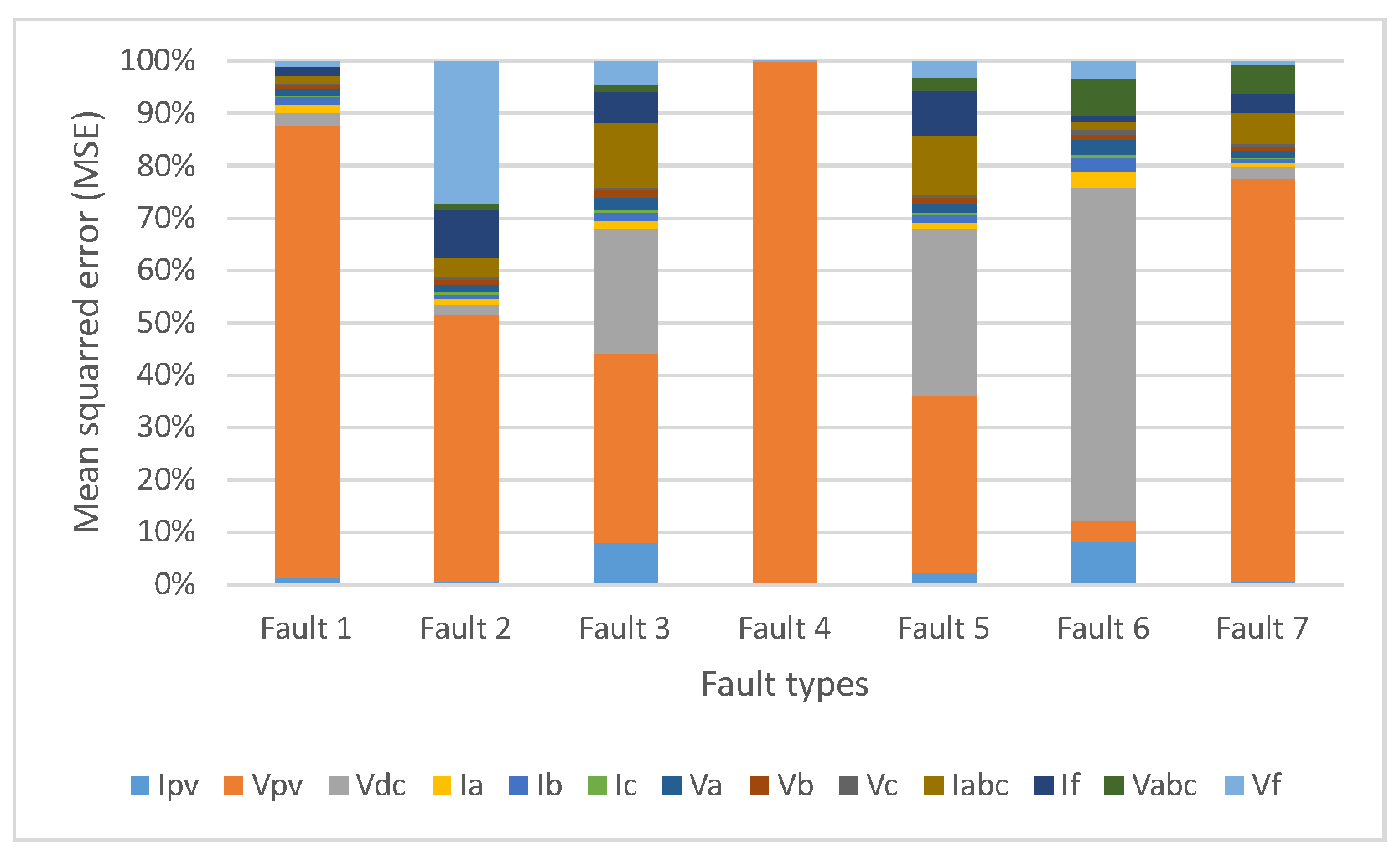
Table 7 presents the individual feature reconstruction errors for the test data of faulty and non-faulty parts. It is apparent from
Table 7 that the feature Vpv is responsible for causing faults in the PV array for all faults except Fault 6, while Vdc causes the system to be faulty under Fault 6. However, Vdc also contributes to fault types 5 and 3. This analysis is further supported by
Figure 2, where the KS test is used to identify the faulty features in the original dataset.
Figure 5 graphically illustrates the individual reconstruction error for the GCN VAE. This figure illustrates that the feature Vpv contributes to making the solar array faulty for fault types 1, 2, 3, 4, 5, and 7, while Vdc contributes to fault types 3, 5, and 6.


 ,
, 


