Coordinated Motion Control of Mobile Self-Reconfigurable Robots in Virtual Rigid Framework

Abstract

This paper presents a control method for the coordinated motion of a mobile self-reconfigurable robotic system. By utilizing a virtual rigid framework, the system ensures that its configuration remains stable and intact, while enabling modular units to collaboratively track the required trajectory and velocity for mobile tasks. The proposed method generates a virtual rigid structure with a specific configuration and introduces an optimized controller with dynamic look-ahead distance and adaptive steering angle. This controller calculates the necessary control parameters for the virtual rigid structure to follow the desired trajectory and speed, providing a unified reference framework for the coordinated movement of the module units. A coordination controller, based on kinematics and adaptive sliding mode control, is developed to enable each module to track the motion of the virtual rigid structure, ensuring the entire robotic system follows the target path while maintaining an accurate configuration. Extensive simulations and experiments under various configurations, robot numbers, and environmental conditions demonstrate the effectiveness and robustness of the proposed method. This approach shows strong potential for applications in smart factories, particularly in material transport and assembly line supply.

1. Introduction

Traditional robots are typically customized from the top down to meet specific task requirements and operate in controlled environments. Most are designed to perform particular tasks and lack the flexibility to adapt to changes in the demands of tasks or working environments. This conventional approach to robot design suffers from several issues, including limited functionality, a restricted working environment, poor scalability, and high redevelopment costs. For example, in smart factories, common tasks such as material transportation and assembly line supply are often addressed by Automatic Guided Vehicle (AGV) solutions. However, a single AGV model usually cannot meet the performance needed for the transportation of products of varying sizes and weights. Consequently, factories must deploy multiple AGV models, which increases both the investment and maintenance costs. Moreover, AGVs typically operate in flat, clean, and uniform environments, and are often unable to handle task requirements that involve environmental changes, such as transitioning from indoor to outdoor spaces. Therefore, researchers aim to enhance robots by reducing the manufacturing costs and simplifying their mechanical structure while simultaneously increasing their functionality and improving the flexibility and scalability of the system to handle diverse working environments and task requirements.

Self-reconfigurable robotic systems [1,2,3,4] offer an improved solution to the aforementioned challenges. These systems can alter their configuration by rearranging the connections between the internal module units, thus breaking free from the structural limitations of traditional robots. This allows them to adapt to changes in tasks or working environments [5]. Additionally, due to the uniformity in the design of module units, these systems offer interchangeability between modules, which ensures good robustness and cost-efficiency at the system level. Mobile robotic systems composed of multiple physically connected module units [6,7,8,9] should operate as a unified whole while maintaining the required system configuration. However, the physical connections between modules mean that the overall mobility and controllability of the system are influenced by the interactions between modules, as well as the physical constraints of the individual module units. To achieve consistent movement, it is necessary to coordinate their individual actions. Therefore, this paper focuses on a specific issue addressed in the research of mobile self-reconfigurable robotic (MSRR) systems: coordinated motion control.

In recent years, researchers have conducted studies on the coordinated motion control of mobile self-reconfigurable robotic systems. An implicit information method combined with the leader–follower approach was used to coordinate a group of rigidly connected surface vessels for trajectory tracking tasks in a planar water environment [10]. However, this method requires the structure to be centrally symmetric, making it unsuitable for coordinating arbitrary configurations. A velocity controller is designed to regulate the platform’s kinematic and hardware constraints, enabling it to satisfy the kinematic requirements during transitions [4]. However, the robustness of this method requires further exploration. A backstepping control strategy that combines robust control with Proportional–Integral–Derivative (PID) control was proposed [11], ensuring the system’s overall path-tracking performance. However, this method does not consider the impact of environmental resistance on dynamics. References [12,13] use artificial evolution to synthesize neural network controllers, enabling the smooth movement of the s-bots system. However, this method requires a large number of iterations, leading to the consumption of significant computational resources and making it difficult to ensure the real-time responsiveness of the control system. In reference [14], a dynamic control law based on the Lyapunov method is proposed, but the model does not account for the nonholonomic constraints of the module units. Some coordinated motion algorithms do not take into account the uncertainties arising from dynamic changes in the external environment [15,16]. Furthermore, in the MSRR system, individual unit modules function as mobile robotic entities capable of independent motion. During the system’s coordinated movement, path-tracking for these individual modules is a critical task to ensure adherence to predefined trajectories. The Pure Pursuit Controller (PPC), a trajectory tracking algorithm based on geometric methods, has been widely utilized in path-tracking tasks for mobile systems, including robots and autonomous vehicles [17,18]. The PPC operates by selecting a look-ahead point on the target path and continuously adjusting the robot’s speed and steering angle to align its motion direction with this point, thereby achieving effective path-tracking. However, this algorithm is highly sensitive to path curvature changes, often resulting in poor performance on high-curvature paths or sharp turns. Moreover, tuning the look-ahead distance is typically performed using empirical methods, requiring manual adjustments to accommodate varying path and velocity requirements [19]. References [20,21,22] applied the Stanley controller to tackle the path-tracking problem in robots. This method relies on the lateral error, which is the distance between the robot’s front axle center and the nearest point on the reference path, as a feedback signal. A nonlinear function computes the steering angle for the front wheels, enabling the robot to follow the predefined path. However, the Stanley controller encounters limitations on high-curvature paths, such as sharp turns, where it may fail to produce sufficiently large steering angles, resulting in increased tracking deviations. References [23,24,25,26] utilized improved PID controllers to adjust the robot’s motion based on path and angle deviations during movement. These controllers feature a simple structure and are easy to implement. References [27,28,29,30] applied the Model Predictive Controller (MPC), which uses optimization algorithms to predict the robot’s trajectory over several future steps and selects the optimal control inputs to minimize tracking errors. This method accounts for the kinematic and dynamic constraints of the robot, achieving high control precision. However, it has high computational complexity and stringent hardware requirements. Additionally, studies have reported the use of Sliding Mode Controllers (SMCs) [31,32] and Fuzzy Logic Controllers (FLCs) [33,34] to address the path-tracking problem in mobile robots.

This study focuses on the coordinated motion control of a mobile self-reconfigurable robotic system. The module units are connected using mechanisms that allow for a certain degree of rotational freedom in the plane, unlike some systems that are completely rigid and lack any degree of freedom [10]. This design provides the system with a redundancy adjustment range when subjected to external disturbances, helping to reduce the structural damage or fatigue caused by the concentration of stress. However, it also imposes greater demands on the system’s coordinated motion control. To address these challenges, this paper proposes a coordinated motion control method that ensures that the module units maintain stable relative positions during movement, allowing the robotic system to complete motion tasks along a designated trajectory while maintaining a fixed configuration. It is worth noting that this paper focuses on the coordinated motion of robotic modules within the MSRR system while maintaining a stable configuration. When encountering obstacles such as narrow passages along the path, the system demonstrates adaptability to changing operating conditions through reconfigurable deformation planning to adjust its configuration. Relevant studies on this topic have been addressed in previous work [35]. Specifically, the contributions of this paper are summarized as follows:

(1)

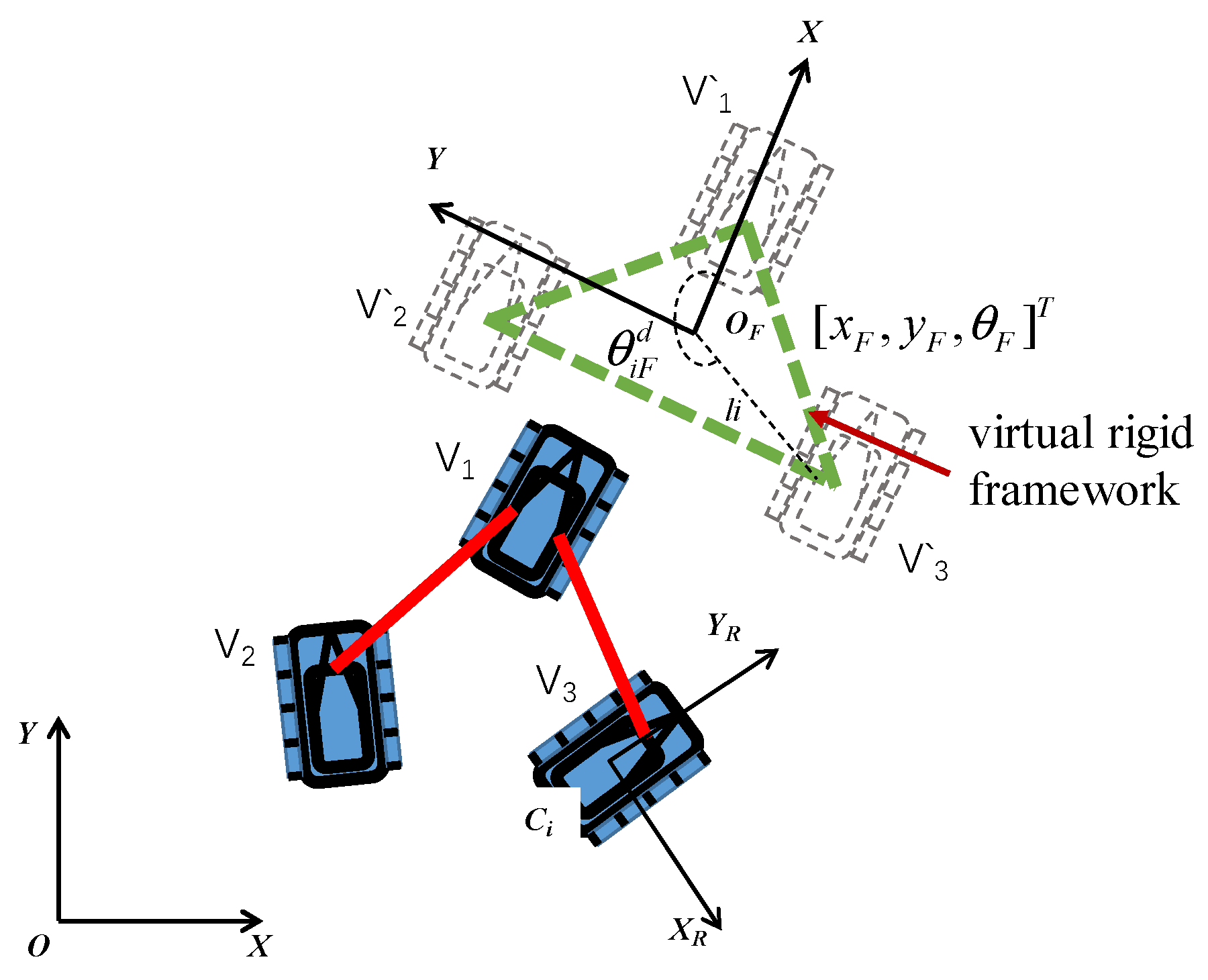
A virtual rigid framework is created to serve as a reference for maintaining the spatial relationships between the module units. An optimized pure pursuit and PID (PPC-PID) controller for the virtual rigid structure is designed to generate the quantity of motion control needed for path-tracking.

(2)

A backstepping-based module unit motion controller that incorporates kinematic and adaptive sliding mode control is designed; this is accomplished to enable the module units to track the movement of the virtual rigid structure.

The remainder of this paper is organized as follows. Section 2 presents the virtual rigid framework and the motion controller for the virtual rigid structure. Section 3 provides detailed information about the coordinated motion controller. Section 4 validates the simulation and experiment. Section 5 discusses the contributions of this paper and outlines future work.

2. Virtual Rigid Structure Motion Control

2.1. Generation of the Virtual Rigid Structure Under the Virtual Rigid Framework

The virtual rigid framework serves as a geometric and kinematic reference for the entire system, dictating the spatial relationships between the module units. This framework ensures that the relative positions of the module units are maintained during motion, allowing the system to function as a single, unified entity. The framework is designed with specific constraints that simulate the configuration. The virtual rigid framework XO_FY is established to satisfy the configuration constraints of the system. Each module unit is assigned a corresponding position and orientation within the virtual rigid framework. The position and orientation angle of a specific module unit in the virtual rigid framework are denoted as ${\mathit{p}}_{iF}^d$ and ${\theta }_{iF}^d$, respectively, as illustrated in Figure 1.

The position of a specific module unit in the virtual rigid framework is represented by the following:

$${\mathit{p}}_{iF}^d=\left[\begin{array}{c}{x}_{iF}^d\\ y_{iF}^d\end{array}\right]=\left[\begin{array}{c}{l}_i\cos {\theta }_{iF}^d\\ l_i\sin {\theta }_{iF}^d\end{array}\right]$$

(1)

The multi-robot system can be transformed into a unified entity with a fixed geometric configuration; this is referred to as a virtual rigid structure (VRS). The origin $O_F$ of the virtual rigid framework XO_FY is designated as the virtual center point of the VRS. In the global coordinate system XOY, the state of the VRS can be expressed as ${\mathit{q}}_F={[x_F,y_F,{\theta }_F]}^T$. Under the constraints of the virtual rigid framework, the position of each module unit in the VRS is represented by the following:

$${\mathit{p}}_i^d={\mathit{p}}_F+\mathit{R}({\theta }_F){\mathit{p}}_{iF}^d$$

(2)

where

$$\mathit{R}({\theta }_F)=\left[\begin{array}{cc}\cos {\theta }_F& -\sin {\theta }_F\\ \sin {\theta }_F& \cos {\theta }_F\end{array}\right]$$

For the actual position of a module unit robot ${\mathit{p}}_i$ and its corresponding position within VRS ${\mathit{p}}_i^d$, the following condition must be satisfied in order to maintain the desired configuration during motion:

$$\underset{t\to \infty }{\lim }‖{\mathit{p}}_i-{\mathit{p}}_i^d‖=0,\forall i\in \left\{1,2,\cdots ,N\right\}$$

(3)

2.2. Optimized PPC-PID Controller for VRS

The movement of the VRS provides a unified reference for the coordinated motion of the mobile self-reconfigurable robotic system. In the main task, a predefined path is followed at a specified speed, with the deviation between the actual and desired positions minimized by adjusting the speed and direction. To address the challenge of path-tracking, this paper proposes a hierarchical control structure: the upper layer uses a dynamically optimized Pure Pursuit Controller (PPC) to calculate the steering angle, while the lower layer employs a PID controller to regulate the speed. This division ensures the precise path-tracking of the VRS, as shown in Figure 2.

The core idea of the PPC controller is to identify a tracking point at a look-ahead distance L_d. Using geometric methods, it calculates an arc curve leading to the tracking point, guiding the VRS towards it. As the VRS moves, the tracking point is continuously updated, enabling the VRS to follow the preset path, as illustrated in Figure 3.

The path trajectory of the VRS from its current position $p_F$ to the current tracking point $s_t$ can be determined using a fitted arc curve. Based on the geometric relationships, the curvature ${\kappa }_{pp}$ of the fitted curve can be calculated as follows:

$${\kappa }_{pp}={\displaystyle \frac{1}{R}}={\displaystyle \frac{2\sin \alpha }{L_d}}$$

(4)

Then, the steering angle ${\delta }_F$ required for the VRS to move along the fitted arc curve can be calculated as follows:

$${\delta }_F=\arctan {\kappa }_{pp}$$

(5)

As shown in Equation (4), the size of the look-ahead distance parameter L_d affects the steering angle of the VRS during path-tracking, thereby influencing both the tracking accuracy and motion stability. In this paper, the look-ahead distance L_d is dynamically adjusted based on the VRS’s motion speed $v_F$ and the path curvature $\kappa$, optimizing both the precision and stability of path-tracking. The dynamic adjustment function for L_d is constructed as follows:

$$L_d(v_F,\kappa )=(k_v{v}_F+L_0){\displaystyle \frac{k_{\kappa }\tanh (\kappa )}{\kappa }}$$

(6)

where $k_v,k_{\kappa }$ represent the speed proportional coefficient and curvature proportional coefficient, respectively. L₀ denotes the base look-ahead distance. To estimate the curvature $\kappa$, a small-range estimation method can be used; this involves selecting the three forward path points $\{s_j,s_{j+1},s_{j+2}\}$ that are closest to the VRS’s current position $p_F$.

In the hierarchical control structure, the lower-layer PID controller governs the motion of the VRS based on the desired velocity $v_{Fd}$ and the steering angle ${\delta }_F$ command that is output from the upper-layer PPC controller. The control input is the error between the actual velocity and the desired velocity during the VRS’s motion. This can be expressed as $e(k)=v_{Fd}(k)-v_F(k)$. To maintain stability during motion, it is necessary to reduce the speed in areas that have larger steering angles ${\delta }_F$ to prevent understeering. The heuristic function for $v_{Fd}$ based on ${\delta }_F$ can be designed as follows:

$$v_{Fd}=\max \{v_{Fd\min },v_{Fd\max }{e}^{-k_{\delta }\left|{\delta }_F\right|}\}$$

(7)

The angular velocity ${\omega }_F$ of the VRS is given as ${\omega }_F=v_F\tan {\delta }_F$.

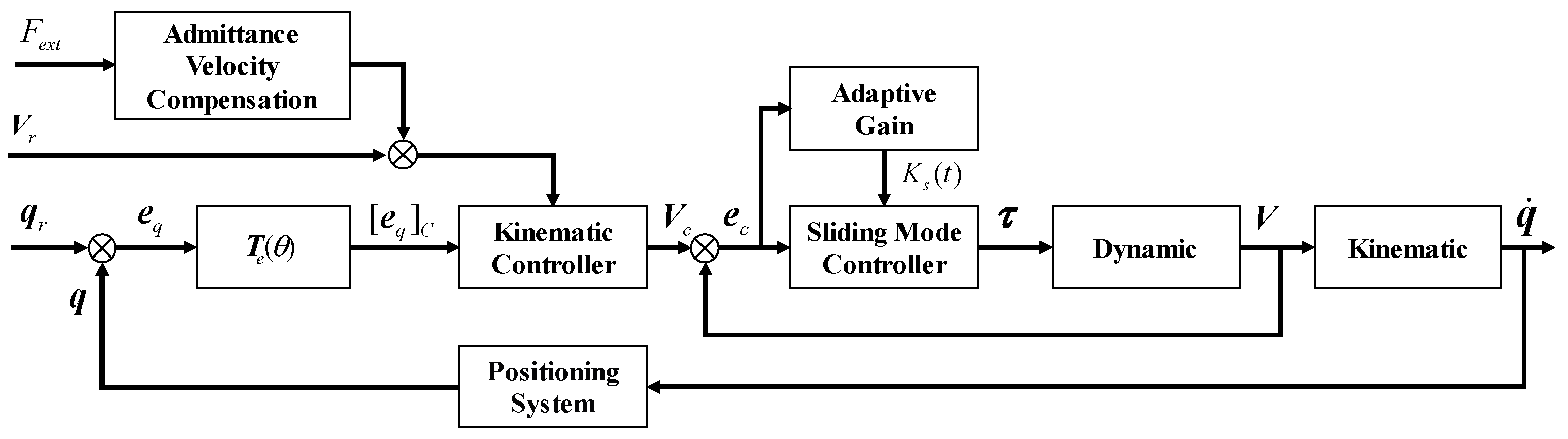
3. Coordinated Motion Controller Based on Kinematics and Adaptive Sliding Mode Control

Under the constraints of the virtual rigid framework, the motion states $v_F$ and ${\omega }_F$ of the VRS provide a unified motion reference for all module units within the framework. Then, through geometric relationships, the corresponding velocities and positions are distributed to each module unit that forms the VRS, establishing their respective desired motion states. By applying motion control strategies, each module unit tracks its desired state, thereby achieving coordinated motion for the entire system. This control process is illustrated in Figure 4.

During the overall coordinated motion of the configuration, the desired velocity of each module unit is determined by the VRS. By differentiating Equation (2), the desired velocity can be obtained:

$$\left[\begin{array}{c}{\dot{x}}_r\\ {\dot{y}}_r\end{array}\right]=\left[\begin{array}{c}{\dot{p}}_{ix}^d\\ {\dot{p}}_{iy}^d\end{array}\right]=\left[\begin{array}{c}{v}_F\cos {\theta }_F-l_i{\omega }_F\sin ({\theta }_F+{\theta }_{iF}^d)\\ v_F\sin {\theta }_F+l_i{\omega }_F\cos ({\theta }_F+{\theta }_{iF}^d)\end{array}\right]$$

(8)

When the mobile self-reconfigurable robotic system moves as a unified entity, external environmental disturbances can cause differences in the relative motion between the module units. These motion differences manifest as forces acting on the connection mechanisms, increasing internal stress within the system and causing the module units to counteract each other, which negatively impacts the stability and coordination of the system during its overall motion. Assuming that the interaction force $F_{ext}$ between the connected module units and its relative angle $\phi$ are measurable, a compliant velocity compensation term is generated in response to the measured force by using an admittance control strategy; this adjusts the desired velocities of the module units across the entire system, thereby reducing the internal force coupling. At the sampling time Δt, the velocity compensation $v_a$ of the module unit, in response to the interaction forces exerted on the connection mechanism, can be obtained as follows:

$$v_a=M_a^{-1}(F_{ext}-B_{a}v)\Delta t$$

(9)

After adding the velocity compensation term, Equation (8) can be rewritten as follows:

$$\left[\begin{array}{c}{\dot{x}}_r\\ {\dot{y}}_r\end{array}\right]=\left[\begin{array}{c}{v}_F\cos {\theta }_F-l_i{\omega }_F\sin ({\theta }_F+{\theta }_{iF}^d)\\ v_F\sin {\theta }_F+l_i{\omega }_F\cos ({\theta }_F+{\theta }_{iF}^d)\end{array}\right]+\left[\begin{array}{c}{v}_a\cos \phi \\ v_a\sin \phi \end{array}\right]$$

(10)

Further, the desired linear velocity, angular velocity, and heading angle for each module unit can be expressed as follows:

$$v_r=\sqrt{{\dot{x}}_r^2+{\dot{y}}_r^2}$$

(11)

$${\omega }_r={\omega }_F$$

(12)

$${\theta }_r=\arctan 2({\dot{y}}_r,{\dot{x}}_r)$$

(13)

By combining Equations (2) and (11)–(13), when using the VRS as the tracking target, the desired motion state of a module unit can be expressed as follows:

$${\mathit{q}}_r=\left[\begin{array}{c}{x}_r\\ y_r\\ {\theta }_r\end{array}\right],{\mathit{V}}_r=\left[\begin{array}{c}{v}_r\\ {\omega }_r\end{array}\right]$$

(14)

The module unit studied in this paper uses a tracked differential drive system, which introduces nonholonomic constraints and nonlinear friction. The kinematic and dynamic models of the system are described as follows:

$$\dot{\mathit{q}}=\mathit{S}(\mathit{q})\mathit{V}$$

(15)

$$\overline{\mathit{M}}(\mathit{q})\dot{\mathit{V}}+\overline{\mathit{C}}(\mathit{q},\dot{\mathit{q}})\mathit{V}+\overline{\mathit{f}}=\overline{\mathit{B}}\mathit{\tau }$$

(16)

For the nonholonomic system described by Equations (15) and (16), the kinematic and dynamic models depict the system’s behavior at different levels, forming a cascaded system. This section employs the backstepping recursive control design method, which divides the nonlinear system into two control sub-layers. By recursively designing virtual control inputs, the control error in each layer is stabilized, eventually yielding the overall control input for the system. The procedure consists of the following two steps:

(1)

Based on the kinematic model of the module unit, a velocity control input ${\mathit{V}}_c$ is designed. This ensures that under the desired velocity ${\mathit{V}}_r$, the pose error between the module unit’s actual pose and the desired pose converges to zero.

(2)

Based on the velocity tracking error, a dynamic controller is designed to ensure that the module unit’s actual velocity $\mathit{V}$ converges to the control velocity ${\mathit{V}}_c$ determined by the kinematic control layer.

The control structure of the coordinated motion controller proposed in this paper is illustrated in Figure 5.

3.1. Kinematic Controller Based on an Error Model

In the robot’s local coordinate system, the pose error between the actual pose and the desired pose of the module unit is described as follows:

$${[{\mathit{e}}_q]}_C={\left[\begin{array}{c}{e}_x\\ e_y\\ e_{\theta }\end{array}\right]}_C=\left[\begin{array}{ccc}\cos \theta & \sin \theta & 0\\ -\sin \theta & \cos \theta & 0\\ 0& 0& 1\end{array}\right]\left[\begin{array}{c}{x}_r-x\\ y_r-y\\ {\theta }_r-\theta \end{array}\right]={\mathit{T}}_e{\mathit{e}}_q$$

(17)

Since the transformation matrix ${\mathit{T}}_e$ is invertible, when ${[{\mathit{e}}_q]}_C\to 0$, ${\mathit{e}}_q\to 0$. Ensuring that ${[{\mathit{e}}_q]}_C$ converges to zero enables the module unit to track its desired pose accurately. By differentiating Equation (17), the pose tracking error model for the module unit can be derived as follows:

$${[{\dot{\mathit{e}}}_q]}_C={\left[\begin{array}{c}{\dot{e}}_x\\ {\dot{e}}_y\\ {\dot{e}}_{\theta }\end{array}\right]}_C=\left[\begin{array}{c}-1\\ 0\\ 0\end{array}\right]v+\left[\begin{array}{c}{e}_y\\ -e_x\\ -1\end{array}\right]\omega +\left[\begin{array}{c}{v}_r\cos e_{\theta }\\ v_r\sin e_{\theta }\\ {\omega }_r\end{array}\right]$$

(18)

It is assumed that, at all times, $v_r>0$ and is bounded and that ${\omega }_r$ is also bounded. To ensure that the module unit reaches pose error convergence at the desired velocity ${\mathit{V}}_r$, the control velocity ${\mathit{V}}_c$ is designed. A typical Lyapunov function can be constructed as follows:

$$W_1={\displaystyle \frac{1}{2}}(e_x^2+e_y^2)+{\displaystyle \frac{1}{K_y}}(1-\cos e_{\theta })$$

(19)

Clearly, in Equation (19), when $K_y>0$, $W_1\ge 0$. When combining this with Equation (18), differentiating the Lyapunov function (19) yields the following:

$$\begin{array}{cc}\hfill {\dot{W}}_1& ={\dot{e}}_x{e}_x+{\dot{e}}_y{e}_y+{\displaystyle \frac{1}{K_y}}{\dot{e}}_{\theta }\sin e_{\theta }\hfill \\ & =-e_x(v_c-v_r\cos e_{\theta })-\sin e_{\theta }({\displaystyle \frac{{\omega }_c-{\omega }_r}{K_y}}-v_r{e}_y)\hfill \end{array}$$

(20)

To ensure the system’s asymptotic stability, let ${\dot{W}}_1\le 0$. Under this condition, the control input ${\mathit{V}}_c$ can be derived as follows:

$${\mathit{V}}_c=\left[\begin{array}{c}{v}_c\\ {\omega }_c\end{array}\right]=\left[\begin{array}{c}{v}_r\cos e_{\theta }+K_x{e}_x\\ {\omega }_r+v_r\left(K_y{e}_y+K_{\theta }\sin e_{\theta }\right)\end{array}\right]$$

(21)

where $K_x, K_y, K_{\theta }$ are positive constants.

3.2. Adaptive Sliding Mode Dynamic Controller

For the Lagrangian dynamic model of the module unit described by Equation (16), the model contains robot parameters that are difficult to measure accurately, as well as nonlinear friction effects. These factors make it challenging to precisely describe the robot’s dynamic behavior. To address these challenges, adaptive sliding mode control (ASMC) is used to eliminate the velocity tracking error between the actual motion velocity $\mathit{V}$ of the module unit robot and the control input velocity ${\mathit{V}}_c$. The velocity tracking error is defined as ${\mathit{e}}_c=\mathit{V}-{\mathit{V}}_c={[e_{v,}{e}_{\omega }]}^T$.

The adaptive integral sliding mode surface can be described as follows:

$$\mathit{s}(t)={\mathit{e}}_c+K_s(t){\displaystyle {\int }_0^t{\mathit{e}}_c}dt$$

(22)

The adaptive gain parameter $K_s(t)$ is dynamically adjusted based on the velocity tracking error to enhance the adaptive characteristics of the sliding mode surface. The parameter structure can be defined as $K_s(t)=k_{s0}+k_{s1}\left|{\mathit{e}}_c\right|$, where $k_{s0}>0$ is the fixed gain component and $k_{s1}>0$ is a tuning parameter.

By differentiating Equation (22), a function for the change rate of the sliding mode surface is obtained:

$$\dot{\mathit{s}}(t)={\dot{\mathit{e}}}_c+K_s(t){\mathit{e}}_c+k_{s1}\mathrm{sgn}({\mathit{e}}_c){\dot{\mathit{e}}}_c{\displaystyle {\int }_0^t{\mathit{e}}_c}dt$$

(23)

Further considering the dynamics model of the module unit, substituting Equation (16) into Equation (23) yields the following:

$$\dot{\mathit{s}}(t)={\displaystyle \frac{\overline{\mathit{B}}\mathsf{\tau }-\overline{\mathit{C}}\mathit{V}-\overline{\mathit{f}}}{\overline{\mathit{M}}}}-{\dot{\mathit{V}}}_c+K_s(t){\mathit{e}}_c+k_{s1}\mathrm{sgn}({\mathit{e}}_c){\dot{\mathit{e}}}_c{\displaystyle {\int }_0^t{\mathit{e}}_c}dt$$

(24)

The equivalent control term ensures that the system remains on the sliding mode surface in finite time, meaning that when $s(t)=0$, $\dot{s}(t)=0$. Under this condition, the equivalent control term can be described as follows:

$${\mathsf{\tau }}_{eq}={\displaystyle \frac{[{\dot{\mathit{V}}}_c-K_s(t){\mathit{e}}_c-k_{s1}\mathrm{sgn}({\mathit{e}}_c){\dot{\mathit{e}}}_c{\displaystyle {\int }_0^t{\mathit{e}}_c}dt]\overline{\mathit{M}}+\overline{\mathit{C}}\mathit{V}+\overline{\mathit{f}}}{\overline{\mathit{B}}}}$$

(25)

Due to the presence of model uncertainties and external disturbances during the motion of the module units, the system state may deviate from the sliding mode surface. To compensate for this, a switching control term is designed as follows:

$${\mathsf{\tau }}_{sw}=-\gamma \mathrm{sat}(\mathit{s},\mathsf{\epsilon })$$

(26)

The switching control term ${\mathsf{\tau }}_{sw}$ is defined using a saturation function $\mathrm{sat}(s,\epsilon )$, which replaces the sign function to avoid excessive chattering near the sliding surface. The parameter ${\mathsf{\epsilon }}_{2\times 1}$ is a small positive constant matrix that defines the thickness of the boundary layer around the sliding surface. $\gamma >0$ is the switching control gain.

By combining the equivalent control term (25) and the switching control term (26), the adaptive sliding mode controller for the coordinated motion of the module unit can be formulated as follows:

$$\mathsf{\tau }={\mathsf{\tau }}_{eq}+{\mathsf{\tau }}_{sw}$$

(27)

3.3. Stability Analysis

To perform the stability analysis of the controller described by Equations (21) and (27), the Lyapunov function is constructed as follows:

$$L=L_1+L_2$$

(28)

where

$$L_1={\displaystyle \frac{1}{2}}(e_x^2+e_y^2)+{\displaystyle \frac{1}{K_y}}(1-\cos e_{\theta })$$

(29)

$$L_2={\displaystyle \frac{1}{2}}{\mathit{s}}^T\mathit{s}$$

(30)

The stability of Equation (29) has already been proven in Section 3.1, where ${\dot{L}}_1\le 0$. By differentiating Equation (30) and substituting Equations (23)–(27), the following is yielded:

$$\begin{array}{cc}{\dot{L}}_2& ={\mathit{s}}^T\dot{\mathit{s}}\hfill \\ & ={\mathit{s}}^T\left[{\displaystyle \frac{\overline{\mathit{B}}\mathsf{\tau }-\overline{\mathit{C}}\mathit{V}-\overline{\mathit{f}}}{\overline{\mathit{M}}}}-{\dot{\mathit{V}}}_c+K_s(t){\mathit{e}}_c+k_{s1}\mathrm{sgn}({\mathit{e}}_c){\dot{\mathit{e}}}_c{\displaystyle {\int }_0^t{\mathit{e}}_c}dt\right]\hfill \\ & =-\gamma {\mathit{s}}^T\mathrm{sat}(\mathit{s},\mathsf{\epsilon })\overline{\mathit{B}}{\overline{\mathit{M}}}^{-1}\le 0\hfill \end{array}$$

(31)

Clearly, $\dot{L}\le 0$ holds and $\dot{L}=0$ if and only if ${[{\mathit{e}}_q]}_C=\mathit{0}$, which means that $\dot{L}$ is negative definite. The above analysis demonstrates that under the action of the coordinated motion controller, the system achieves asymptotic stability. In other words, the following holds: $\underset{t\to \infty }{\lim }\mathit{s}(t)=0,\underset{t\to \infty }{\lim }\left(\mathit{q}-{\mathit{q}}_r\right)=0$.

4. Simulation and Experiment Analysis

The implementation of the control program and coordinated motion simulation for a mobile self-reconfigurable robot system is undertaken in Python 3.8. The sampling rate of the simulation is set to 10 Hz. The objective is to enable the robot system to move as a whole along a given desired path while maintaining a constant configuration, ensuring that the overall position and orientation of the structure are always under control. Additionally, the desired velocity of the structure during straight-line motion is also regulated throughout the process. Then, the experimental verification is conducted to demonstrate the comprehensiveness of the proposed control method.

4.1. Simulation of VRS Motion

To verify the effectiveness of the PPC-PID controller for the path-tracking control of the VRS designed in Section 2, a simulation is conducted. A desired path with a gradually increasing curvature is designed to test the optimization effect of the dynamic look-ahead distance and steering angle adaptation. The parametric equation for the path is given as follows:

$$\left\{\begin{array}{l}x(t)=t\\ y(t)={\displaystyle \frac{1}{2}}t\sin ({\displaystyle \frac{t}{10}})\end{array}\right.$$

(32)

The desired motion speed of the VRS is set to 5 m/s, with an initial pose of ${(0,-3,0.5\pi )}^T$ and an initial velocity of 0 m/s. After multiple parameter adjustments, the PPC-PID controller parameters are set as follows: $L_0=2$, $k_v=0.12$, $k_{\kappa }=0.9$, $k_{\delta }=1$, $k_p=1.9$, $k_i=0.01$.The path-tracking simulation results are shown in Figure 6.

The relationship between the dynamic look-ahead distance L_d, motion speed $v_F$, and path curvature $\kappa$ is shown in Figure 7.

Figure 6a demonstrates that the VRS successfully tracks the given desired trajectory using the designed PPC-PID-optimized controller. Figure 6b shows the adjustment of the VRS’s desired motion speed according to the path curvature. Figure 7 illustrates the variation in the dynamic look-ahead distance with respect to the speed and path curvature, aligning with the design expectations.

To compare the static look-ahead parameter PPC method used in Reference [19] and highlight the improvements in tracking performance achieved through the optimization of a dynamic look-ahead distance, path-tracking simulations under static look-ahead parameters were conducted, as presented in Figure 8.

Figure 8a,b show the path-tracking performance using the controller in Reference [19], as well as the velocity and steering angle variation curves, when using smaller and larger static look-ahead distance parameters, respectively. By comparing these results with the simulations performed using dynamic look-ahead distance parameters in Figure 6, the following can be observed: when a smaller static look-ahead distance is used, the path-tracking error is reduced, but the steering angle changes more frequently. When a larger static look-ahead distance is used, the steering angle variation becomes smoother, but the path-tracking error increases. In contrast to Ref. [19], the control results using dynamic look-ahead distance parameters show a balance between the path-tracking accuracy and the smoothness of the steering angle adjustments, leading to a superior path-tracking performance.

4.2. Simulation of Coordinated Motion

To evaluate the feasibility and robustness of the proposed coordinated motion controller, two sets of simulation tests were designed. In the first test, three robots formed an arrow-shaped configuration and navigated along a sinusoidal oscillating involute parameter curve. In the second test, nine robots formed a cross-shaped configuration and followed an eight-shaped curve. An arrow-shaped configuration consisting of three modular units is set up, with corresponding parameters under the virtual rigid framework denoted as $l_i=(0,5,5),{\theta }_{iF}^d=(0,{\displaystyle \frac{2}{3}}\pi ,-{\displaystyle \frac{5}{6}}\pi )$. The units of l and θ are meters (m) and radians (rad), respectively. The desired trajectory for the motion reference is given by Equation (32). The initial poses of the modular units in global frame are ${[5,10,0]}^T$, ${[-2.5,10+2.5\sqrt{3},{\displaystyle \frac{2\pi }{3}}]}^T$, ${[-2.5,10-2.5\sqrt{3},-{\displaystyle \frac{2\pi }{3}}]}^T$, while the VRS’s pose is ${[0,10,0]}^T$. Each module starts with an initial velocity of 0 m/s and an initial angular velocity of 0 rad/s, with the desired straight-line motion velocity set to 5 m/s. The controller-related parameters are set as follows: $K_x=0.6$, $K_y=3.2$, $K_{\theta }=0.8$, $k_{s0}=0.1$, $k_{s1}=0.01$, $\gamma =2.1$. The system’s coordinated motion simulation results for the trajectory are shown in Figure 9.

In Figure 9a, the trajectory tracking performance of each modular unit is shown to align with the reference trajectory. The deviation observed at the turns is attributed to the large turning radius of the VRS required to maintain the configuration, along with the high curvature during steering. The system’s motion speed decreases accordingly at these points, and the resulting deviation remains within a reasonable tracking range. The tracking errors for each modular unit are presented in Figure 9b. The velocity curves of the center of the VRS and each modular unit are shown in Figure 9c. The velocity error curves are presented in Figure 9d.

To further demonstrate the scalability and robustness of the proposed method, the number of modular units is increased to nine to form a cross-shaped configuration, which is then tasked with tracking more complex trajectory paths. The figure-eight parameter curve, a trajectory commonly employed in studies of path-tracking problems for mobile robots, is selected as the test path. This curve is particularly effective for evaluating the smoothness and control accuracy of path-tracking algorithms, especially under scenarios that demand frequent acceleration and deceleration. The desired trajectory for the motion reference is defined as follows: $x(t)=50\sin (0.05t),y(t)=20\sin (0.1t)$. The corresponding parameters of cross-shaped configuration under the virtual rigid framework is denoted as $l_i=(0,1,2,1,2,1,2,1,2),{\theta }_{iF}^d=(0,0,0,{\displaystyle \frac{1}{2}}\pi ,{\displaystyle \frac{1}{2}}\pi ,\pi ,\pi ,-{\displaystyle \frac{1}{2}}\pi ,-{\displaystyle \frac{1}{2}}\pi )$. The initial poses of the modular units in global frame are as follows: ${[2,5,0]}^{\mathrm{T}}$, ${[3,5,0.1\pi ]}^{\mathrm{T}}$, ${[4,5,-0.1\pi ]}^{\mathrm{T}}$, ${[2,6,0]}^{\mathrm{T}}$, ${[2,7,0]}^{\mathrm{T}}$, ${[1,5,0.1\pi ]}^{\mathrm{T}}$, ${[0,5,-0.1\pi ]}^{\mathrm{T}}$, ${[2,4,0]}^{\mathrm{T}}$, and ${[2,3,0]}^{\mathrm{T}}$, while the VRS’s pose is ${[2,5,0]}^{\mathrm{T}}$. Each module starts with an initial velocity of 0 m/s and an initial angular velocity of 0 rad/s, with the desired straight-line motion velocity set to 1 m/s. To further assess the robustness of the coordinated motion controller, motion velocity error noise was introduced in the simulation. Speed noise with a distribution of −0.25 m/s was introduced during the 64 s simulation period. The system’s coordinated motion simulation results are shown in Figure 10.

The simulation results indicate that, after an initial adjustment phase, the system successfully stabilized and tracked the desired trajectory, with the tracking error maintaining a consistent and steady level, as depicted in Figure 10a,b. As shown in Figure 10c,d, when the system approaches a turn in the path, the reference speed decreases, and each modular unit must adjust its speed accordingly to accommodate the overall system’s turning motion. As the system stabilizes, the velocity errors converge, demonstrating a good tracking performance.

To further evaluate the performance of the controller designed in this study, a comparison was conducted with the Individual Steering Velocity Controller based on the PID control method described in [4]. The parameters of the PID controller were configured as follows: $kp=0.56$, $ki=0.098$, $kd=0.005$. The simulation tracking errors results of Reference [4] are presented in Figure 11.

By analyzing Figure 10b and Figure 11a, it can be observed that the proposed control method achieves significantly smaller VRS tracking errors—approximately 10% of those reported in [4]—while delivering smoother performance when the target velocity changes in response to the path curvature. Once the disturbances dissipate, the system quickly stabilizes and continues to operate seamlessly. Similarly, a comparison of Figure 10d and Figure 11b reveals that the proposed control method produces smaller velocity errors under varying target velocities influenced by the path curvature. Additionally, it effectively smooths and suppresses disturbances caused by instantaneous velocity changes. In contrast, the method described in [4] exhibits more frequent oscillations in velocity adjustments under comparable conditions. The simulation results confirm that the controller developed in this study exhibits superior adaptability and robustness, especially in handling variations in target velocity induced by changes in the path curvature.

4.3. Experimental Verification

In this subsection, the effectiveness of the proposed method is validated through experiments conducted using three MMRP robots [36]. Each robot independently estimates its states, including position and velocity, with the aid of an onboard Ultra-Wideband (UWB) system. UWB anchors were strategically positioned at the four vertices of a rectangular experimental area, while the robots were equipped with integrated UWB tags. The UWB module employed in the experiment also features a built-in IMU (Inertial Measurement Unit), enabling accurate velocity measurement. To validate the robustness of the controller in handling varying numbers of robots, configurations, and working environments, two sets of experiments were conducted. The first set involved a configuration composed of two modular units arranged in a parallel configuration on a structured, flat surface, as depicted in Figure 12. The second experiment took place in an uneven 20 × 15 m dirt area. During motion, the uneven contact between the robot tracks and the soil, combined with stick-slip effects, introduced nonlinear resistance variations, resulting in random velocity disturbances. Three module units are connected in an arrow-shaped configuration, as shown in Figure 13. In both experiments, each module starts with an initial velocity of 0 m/s and an initial angular velocity of 0 rad/s, with the desired straight-line motion velocity set to 1 m/s. The state measurements are recorded at 10 Hz during the experiments. All the experiments are run five times to ensure repeatability.

Figure 14 and Figure 15 illustrate the tracking performance of the coordinated motion of the system in the first and the second experiment, respectively. It can be seen that the module units are able to track various trajectories in an accurate configuration, as shown in Figure 14a and Figure 15a. By comparing Figure 14b and Figure 15b, it can be observed that the tracking errors of the modular units show no significant variation across both sets of experiments conducted on different types of surfaces. This indicates that the controller is effective in suppressing the friction disturbances introduced by changes in the driving surface. Additionally, when comparing Figure 14d and Figure 15d, the velocity error in the first set of experiments appears relatively unstable. This instability arises because the reference path in the first set contains sharp turns with a large curvature. To accommodate these curvature changes, the PPC-PID controller induces significant velocity fluctuations in the VRS. These fluctuations are consistent with the need for control stability and safety, highlighting the system’s responsiveness to dynamic path conditions. In the first set of experiments, the robot system achieved an average tracking distance error of 0.022 m and an average velocity error of −0.051 m/s. In the second set of experiments, the average tracking distance error was 0.053 m, while the average velocity error was −0.024 m/s.

4.4. Analysis

Through the simulations and experimental tests presented above, the effectiveness of the proposed coordinated motion control method for the mobile self-reconfigurable robotic system under the virtual rigid framework has been demonstrated. Through multiple experiments conducted under two different configurations, varying robot numbers, and different working environments, the effectiveness and robustness of the proposed method have been demonstrated. As shown in the comparison in Section 4.1, the optimized PPC-PID controller developed in this study strikes a balance between path-tracking accuracy and the smoothness of steering angle adjustments, resulting in superior path-tracking performance when compared to the method in Reference [19]. Furthermore, as illustrated in Section 4.2, in contrast to the method presented in Reference [4], the proposed approach integrates robust control with kinematics by employing a backstepping technique to design the motion controller. This integration not only enhances the robustness of the control system but also addresses the limitations in robustness observed in the kinematic controller used in the previous method, thereby improving overall system performance. In contrast to the approach used in reference [10], the coordinated motion control method proposed in this paper does not require symmetry between the individual modules and the overall configuration; this reduces the configuration constraints on the self-reconfigurable robot and enhances the applicability of the control method. Moreover, unlike the approaches discussed in References [11,14,15,16], this method explicitly considers the kinematic constraints of the robot and addresses the nonlinear uncertainties encountered during the motion process.

Through experimental testing, certain limitations of the system were identified. First, the positioning system relies on pre-deployed UWB anchors in the working area, which restricts the system’s ability to be rapidly deployed in uncertain or dynamic environments. This limitation could be addressed in future work by integrating GPS and odometry into the positioning system to enhance flexibility and adaptability. Additionally, when the path includes narrow sections, the virtual rigid framework constraint only permits passage through configuration deformation motion, requiring the overall configuration to change shape [35]. A potential solution to this limitation involves dynamically adjusting the virtual rigid framework constraint parameters while navigating narrow paths. This adjustment could include scaling and fine-tuning the relative angles between modular units, ensuring their connectivity is maintained while allowing the system to adapt to tighter spaces.

5. Conclusions

This paper introduces a control method for the coordinated motion of a mobile self-reconfigurable robot system, enabling the robot to track the trajectory and speed required for mobile tasks while maintaining a fixed and accurate configuration. A virtual rigid framework is designed to constrain the possible relative motion between module units, ensuring the accuracy of the configuration during movement. A PPC-PID-optimized controller, enhanced by a dynamic look-ahead distance and adaptive steering angle, is developed to generate control parameters for the virtual rigid structure, guiding it along the desired trajectory and speed. These control parameters serve as a unified motion reference framework for the coordinated movement of the module units. The control parameters of the virtual rigid structure are distributed to each module as the desired coordinated motion. Using the backstepping approach, a kinematics and adaptive sliding mode coordinated motion controller is designed to ensure that each module tracks the motion state of the virtual rigid structure. The simulation and experiment results confirm that the proposed method enables the mobile self-reconfigurable robot to coordinate motion along the desired trajectory at the various desired speeds while maintaining an accurate configuration. This method enhances the practical applicability of self-reconfigurable robot systems in tasks such as material transportation in smart factories, demonstrating significant potential for application in various domains.

The proposed method currently has certain limitations, including the need for the pre-deployment of UWB base stations before the task begins, as well as its inability to quickly and effectively handle narrow obstacles along the path. Future work could focus on machine-learning-based online parameter estimation, which would enhance the real-time accuracy of key parameters used by the modular robots, as discussed in Section 3. Additionally, exploring the design of a dynamic virtual rigid framework that adapts to environmental changes could provide more flexibility. By adjusting specific parameters, the system’s configuration could be fine-tuned while maintaining connectivity, allowing the robots to effectively navigate narrow or constrained environments. Furthermore, the integration of Global Positioning System (GPS) and IMU sensors could be investigated to improve the system’s navigation accuracy, offering more robust performance across varied and unpredictable environments.

References

1. Tu, Y.; Lam, T.L. Configuration Identification for a Freeform Modular Self-reconfigurable Robot-Freesn. IEEE Trans. Robot. 2023, 39, 4636–4652. [Google Scholar] [CrossRef]
2. Daudelin, J.; Jing, G.; Tosun, T.; Yim, M.; Kress-Gazit, H.; Campbell, M. An Integrated System for Perception-Driven Autonomy with Modular Robots. Sci. Robot. 2018, 3, 31. [Google Scholar] [CrossRef] [PubMed]
3. O’Grady, R.; Christensen, A.L.; Dorigo, M. SWARMORPH: Multirobot Morphogenesis Using Directional Self-Assembly. IEEE Trans. Robot. 2009, 25, 738–743. [Google Scholar] [CrossRef]
4. Shi, Y.; Elara, M.R.; Le, A.V.; Prabakaran, V.; Wood, K.L. Path Tracking Control of Self-Reconfigurable Robot hTetro with Four Differential Drive Units. IEEE Robot. Autom. Lett. 2020, 5, 3998–4005. [Google Scholar] [CrossRef]
5. Seo, J.; Paik, J.; Yim, M. Modular Reconfigurable Robotics. Annu. Rev. Control. Robot. Auton. Syst. 2019, 2, 63–88. [Google Scholar] [CrossRef]
6. O’Grady, R.; Groß, R.; Christensen, A.L.; Dorigo, M. Self-assembly strategies in a group of autonomous mobile robots. Auton. Robot. 2010, 28, 439–455. [Google Scholar] [CrossRef]
7. Liu, C.; Lin, Q.; Kim, H.; Yim, M. SMORES-EP, a Modular Robot with Parallel Self-Assembly. Auton. Robot. 2023, 47, 211–228. [Google Scholar] [CrossRef]
8. Zhao, D.; Lam, T.L. SnailBot: A Continuously Dockable Modular Self-Reconfigurable Robot Using Rocker-Bogie Suspension. In Proceedings of the IEEE International Conference on Robotics and Automation, Philadelphia, PA, USA, 23–27 May 2022; Institute of Electrical and Electronics Engineers Inc.: Piscataway, NJ, USA, 2022; pp. 4261–4267. [Google Scholar]
9. Wei, H.; Chen, Y.; Tan, J.; Wang, T. Sambot: A self-assembly modular robot system. IEEE/ASME Trans. Mechatron. 2011, 16, 745–757. [Google Scholar] [CrossRef]
10. Wang, W.; Wang, Z.; Mateos, L.; Huang, K.W.; Schwager, M.; Ratti, C.; Rus, D. Distributed motion control for multiple connected surface vessels. In Proceedings of the IEEE International Conference on Intelligent Robots and Systems, Las Vegas, NV, USA, 24–29 October 2020; pp. 11658–11665. [Google Scholar]
11. Parween, R.; Vega Heredia, M.; Rayguru, M.M.; Enjikalayil Abdulkader, R.; Elara, M.R. Autonomous Self-Reconfigurable Floor Cleaning Robot. IEEE Access 2020, 8, 114433–114442. [Google Scholar] [CrossRef]
12. Baldassarre, G.; Trianni, V.; Bonani, M.; Mondada, F.; Dorigo, M.; Nolfi, S. Self-organized coordinated motion in groups of physically connected robots. IEEE Trans. Syst. Man Cybern. Part B Cybern. 2007, 37, 224–239. [Google Scholar] [CrossRef]
13. Trianni, V.; Nolfi, S.; Dorigo, M. Cooperative hole avoidance in a swarm-bot. Robot. Auton. Syst. 2006, 54, 97–103. [Google Scholar] [CrossRef]
14. Lee, M.; Li, T.S. Kinematics, dynamics and control design of 4WIS4WID mobile robots. J. Eng. 2015, 2015, 6–16. [Google Scholar] [CrossRef]
15. Hajieghrary, H.; Kularatne, D.; Hsieh, M.A. Cooperative transport of a buoyant load: A differential geometric approach. In Proceedings of the 2017 IEEE/RSJ International Conference on Intelligent Robots and Systems (IROS), Vancouver, BC, Canada, 24–28 September 2017; pp. 2158–2163. [Google Scholar] [CrossRef]
16. Hajieghrary, H.; Kularatne, D.; Hsieh, M.A. Differential Geometric Approach to Trajectory Planning: Cooperative Transport by a Team of Autonomous Marine Vehicles. In Proceedings of the 2018 Annual American Control Conference (ACC), Milwaukee, WI, USA, 27–29 June 2018; pp. 858–863. [Google Scholar] [CrossRef]
17. Wang, R.; Li, Y.; Fan, J.; Wang, T.; Chen, X. A novel pure pursuit algorithm for autonomous vehicles based on salp swarm algorithm and velocity controller. IEEE Access 2020, 8, 66525–166540. [Google Scholar] [CrossRef]
18. AbdElmoniem, A.; Afif, Y.T.; Maged, S.A.; Abdelaziz, M.; Hammad, S. Adaptive pure-pursuit controller based on particle swarm optimization (pso-pure-pursuit). In Proceedings of the 2021 16th International Conference on Computer Engineering and Systems (ICCES), Cairo, Egypt, 15–16 December 2021; pp. 1–6. [Google Scholar]
19. Nawawi, S.W.; Abdeltawab, A.A.A.; Samsuria, N.E.N. Modelling, simulation and navigation of a two-wheel mobile robot using pure pursuit controller. ELEKTRIKA-J. Electr. Eng. 2022, 21, 69–75. [Google Scholar] [CrossRef]
20. AbdElmoniem, A.; Osama, A.; Abdelaziz, M.; Maged, S.A. A path-tracking algorithm using predictive Stanley lateral controller. Int. J. Adv. Robot. Syst. 2020, 17, 1729881420974852. [Google Scholar] [CrossRef]
21. Wang, L.; Zhai, Z.; Zhu, Z.; Mao, E. Path tracking control of an autonomous tractor using improved Stanley controller optimized with multiple-population genetic algorithm. Actuators 2022, 11, 22. [Google Scholar] [CrossRef]
22. Sun, Y.; Cui, B.; Ji, F.; Wei, X.; Zhu, Y. The full-field path tracking of agricultural machinery based on PSO-enhanced fuzzy stanley model. Appl. Sci. 2022, 12, 7683. [Google Scholar] [CrossRef]
23. Xiong, R.; Li, L.; Zhang, C.; Ma, K.; Yi, X.; Zeng, H. Path tracking of a four-wheel independently driven skid steer robotic vehicle through a cascaded NTSM-PID control method. IEEE Trans. Instrum. Meas. 2022, 71, 7502311. [Google Scholar] [CrossRef]
24. Ammar, H.H.; Azar, A.T. Robust path tracking of mobile robot using fractional order PID controller. In Proceedings of the International Conference on Advanced Machine Learning Technologies and Applications (AMLTA2019), Cairo, Egypt, 28–30 March 2019; Springer International Publishing: Berlin/Heidelberg, Germany, 2019; Volume 4, pp. 370–381. [Google Scholar]
25. Algabri, R.; Choi, M.T. Deep-learning-based indoor human following of mobile robot using color feature. Sensors 2020, 20, 2699. [Google Scholar] [CrossRef]
26. Zangina, U.; Buyamin, S.; Abidin, M.S.Z.; Azimi, M.S.; Hasan, H.S. Non-linear PID controller for trajectory tracking of a differential drive mobile robot. J. Mech. Eng. Res. Dev. 2020, 43, 255–270. [Google Scholar]
27. Zuo, Z.; Yang, X.; Li, Z.; Wang, Y.; Han, Q.; Wang, L.; Luo, X. MPC-based cooperative control strategy of path planning and trajectory tracking for intelligent vehicles. IEEE Trans. Intell. Veh. 2020, 6, 513–522. [Google Scholar] [CrossRef]
28. Peicheng, S.; Li, L.; Ni, X.; Yang, A. Intelligent vehicle path tracking control based on improved MPC and hybrid PID. IEEE Access 2022, 10, 94133–94144. [Google Scholar] [CrossRef]
29. Yu, J.; Guo, X.; Pei, X.; Chen, Z.; Zhou, W.; Zhu, M.; Wu, C. Path tracking control based on tube MPC and time delay motion prediction. IET Intell. Transp. Syst. 2020, 14, 1–12. [Google Scholar] [CrossRef]
30. Rokonuzzaman, M.; Mohajer, N.; Nahavandi, S.; Mohamed, S. Model predictive control with learned vehicle dynamics for autonomous vehicle path tracking. IEEE Access 2021, 9, 128233–128249. [Google Scholar] [CrossRef]
31. Cen, H.; Singh, B.K. Nonholonomic wheeled mobile robot trajectory tracking control based on improved sliding mode variable structure. Wirel. Commun. Mob. Comput. 2021, 1, 2974839. [Google Scholar] [CrossRef]
32. Azzabi, A.; Nouri, K. Design of a robust tracking controller for a nonholonomic mobile robot based on sliding mode with adaptive gain. Int. J. Adv. Robot. Syst. 2021, 18, 1729881420987082. [Google Scholar] [CrossRef]
33. Abood, M.S.; Thajeel, I.K.; Alsaedi, E.M.; Hamdi, M.M.; Mustafa, A.S.; Rashid, S.A. Fuzzy Logic Controller to control the position of a mobile robot that follows a track on the floor. In Proceedings of the 2020 4th International Symposium on Multidisciplinary Studies and Innovative Technologies (ISMSIT), Istanbul, Turkey, 22–24 October 2020; pp. 1–7. [Google Scholar]
34. Abdelwahab, M.; Parque, V.; Elbab, A.M.F.; Abouelsoud, A.A.; Sugano, S. Trajectory tracking of wheeled mobile robots using z-number based fuzzy logic. IEEE Access 2020, 8, 18426–18441. [Google Scholar] [CrossRef]
35. Wei, R.; Liu, Y.; Dong, H.; Zhu, Y.; Zhao, J. A Graph-Based Hybrid Reconfiguration Deformation Planning for Modular Robots. Sensors 2023, 23, 7892. [Google Scholar] [CrossRef]
36. Liu, Y.; Wei, R.; Dong, H.; Zhu, Y.; Zhao, J. A designation of modular mobile reconfigurable platform system. J. Mech. Med. Biol. 2020, 20, 2040006. [Google Scholar] [CrossRef]
Figure 1. Schematic diagram of a virtual rigid framework.
Machines 12 00888 g001
Figure 2. The hierarchical control structure of PPC-PID.
Machines 12 00888 g002
Figure 3. Pure pursuit control motion model.
Machines 12 00888 g003
Figure 4. Schematic diagram of the motion process of the module units following a virtual rigid structure.
Machines 12 00888 g004
Figure 5. Structure of coordinated motion controller.
Machines 12 00888 g005
Figure 6. Path-tracking results of the VRS based on PPC-PID control. (a) Path-tracking trajectory of VRS. (b) The relationship between the motion speed and the steering angle of the VRS.
Machines 12 00888 g006
Figure 7. The relationship between the dynamic look-ahead distance, speed, and path curvature.
Machines 12 00888 g007
Figure 8. Path-tracking results under static look-ahead parameters PPC in Reference [19]. (a) Path-tracking results using a small static look-ahead parameter Ld = 1. (b) Path-tracking results using a large static look-ahead parameter Ld = 5.
Machines 12 00888 g008
Figure 9. Coordinated motion simulation results for arrow-shaped configuration. (a) Trajectories of each module unit during the coordinated motion process. (b) The tracking errors for each modular unit. (c) The velocity of each modular unit. (d) The velocity error of each modular unit.
Machines 12 00888 g009
Figure 10. Simulation results of cross-shaped configuration during the coordinated motion process. (a) Trajectories of each module unit during the coordinated motion process. (b) The tracking errors for each modular unit. (c) The velocity of each modular unit. (d) The velocity error of each modular unit.
Machines 12 00888 g010
Figure 11. Tracking errors of PID controller in Reference [4]. (a) The tracking errors for each modular unit. (b) The velocity errors for each modular unit.
Machines 12 00888 g011
Figure 12. A coordinated motion experiment is conducted with two module units arranged in a parallel configuration on flat surface. The desired trajectory is shown by the red dashed lines.
Machines 12 00888 g012
Figure 13. A coordinated motion experiment is conducted with three module units arranged in an arrow-shaped configuration on uneven dirt surface. The desired trajectory is shown by the red dashed lines.
Machines 12 00888 g013
Figure 14. Coordinated motion performance in parallel configuration on flat surface. (a) Trajectories of each module unit during the coordinated motion process. (b) The tracking errors for each modular unit. (c) The velocity of each modular unit. (d) The velocity error of each modular unit.
Machines 12 00888 g014
Figure 15. Coordinated motion performance in arrow-shaped configuration on uneven dirt surface. (a) Trajectories of each module unit during the coordinated motion process. (b) The tracking errors for each modular unit. (c) The velocity of each modular unit. (d) The velocity error of each modular unit.
Machines 12 00888 g015
Disclaimer/Publisher’s Note: The statements, opinions and data contained in all publications are solely those of the individual author(s) and contributor(s) and not of MDPI and/or the editor(s). MDPI and/or the editor(s) disclaim responsibility for any injury to people or property resulting from any ideas, methods, instructions or products referred to in the content.