Coupling Interface Load Identification of Sliding Bearing in Wind Turbine Gearbox Based on Polynomial Structure Selection Technique

Abstract

Sliding bearings are widely used in wind turbine gearboxes, and the accurate identification of coupling interface loads is critical for ensuring the reliability and performance of these systems. However, the space–time coupling nature of these loads makes them difficult to calculate and measure directly. An improved method utilizing the POD decomposition algorithm and polynomial selection technology is proposed in this paper to identify the sliding bearing coupling interface loads. By using the POD decomposition algorithm, the sliding bearing coupling interface loads can be decomposed into the form of a series of independent oil film time history and spatial distribution functions. Then, it can be converted into space–time independent sub-coupled interface load identification in which oil film time history can be transformed into the recognition of a certain order modal load and the corresponding oil film spatial distribution function can be fitted with a set of Chebyshev orthogonal polynomial. To address the ill-posedness caused by the weak correlation between the modal matrix and polynomial options during the identification process, this paper introduces polynomial structure selection technology. Firstly, displacement responses are collected, and a series of modal loads are identified using conventional concentrated load identification methods. Then, the polynomial structure selection technology is applied to select the effective modal shape matrix, using a specific mode load as the oil film time history function. The load ratios of other mode loads to this reference mode load are compared, and the effective Chebyshev orthogonal polynomials are selected based on the error reduction ratio. Finally, multiplying the identified oil film time histories by the corresponding oil film spatial distribution functions yields the coupling interface load. The results of the numerical examples verify the improved method’s rationality and effectiveness.

1. Introduction

The sliding bearing is the most potential support design scheme for the transmission system of high-power wind power gearboxes; it is widely applied in the planetary and parallel stages of gearboxes to replace the high-fault rolling bearings [1,2]. The coupling interface load between sliding bearings with the wind turbine gearbox is affected by the frequent start–stop impact load, yaw moment, wind wheel weight, and unbalanced load on the gearbox. The non-torsional load changes over time, resulting in oil film whirl and oscillation, which is an important basis for monitoring the operation status and fault diagnosis of key components such as wind turbines. However, the flexible gear shaft and complex load conditions from the helical tooth meshes lead to highly complex elastic structure deformation that modifies the lubricant film thickness and pressure distribution [3,4]. The film thickness considering the axial misalignment and thermoelastic deformations at heavy-load and low-speed operating conditions, shown in Figure 1, varies from large to small, and it is different at different spatial positions, the distribution of oil film pressure related to the oil film thickness is also different. So, the coupling interface load of sliding bearing in a wind turbine gearbox exhibits spatiotemporal coupling characteristics that need to be represented by variables in both temporal and spatial dimensions. However, it is difficult to calculate and measure directly due to the variability of position and direction of load in extreme service environments. By contrast, it is more convenient and effective to measure structural responses. Therefore, the distributed dynamic load identification method [5,6,7] coupled with measurable shafting response and characteristics is introduced into the sliding bearing coupling interface load identification.

The coupling interface load of sliding bearings involves both spatial and temporal dimensions and is usually treated as a time–space coupled load. The form of the load is dynamic in time, and the form of the load also presents a certain distribution in space. It is very difficult to directly identify the coupling interface load with time–space coupling characteristics by using the distributed dynamic load identification method. The decoupling [8] and dimension reduction [9] of time–space coupling load is a common method. You and Zhang et al. [10] decouple the composite load of the blade under combined load by using key technologies such as orthogonal load decoupling load and coordinated loading control based on the analysis of blade failure mode and load form. Chen et al. [11] acquire the strain response of the strong coupling boundary measurement points by loading load conditions and disturbance load conditions to the gearbox and decouple the strong coupling load by using Short-Time Fourier Transform (STFT) and the frequency domain based on strain response. Li et al. [12] presented a decoupling and dimension approach for load identification to decouple and reduce the dimension of each load identification point by removing the coupling relationship between each load. Sun and Guo et al. [13] proposed a method for decoupling complex loads into fundamental loads applicable to a test platform. Cao and Sun et al. [14] used the proper orthogonal decomposition method (POD) to identify thermal parameters in heat conduction problems varied with both time and measurement locations. The POD decomposition algorithm [15,16,17] decouples the interface load of sliding bearings, simplifying the representation of two corresponding independent variables: time history and spatial distribution function.

In vibration problems of sliding bearing coupling interface loads, the measured displacement responses are often time-sequential and limited in number. Therefore, it is challenging to comprehensively reflect and identify the discrete values of the spatial distribution function of the load on the sliding bearing coupling interface using limited time-based responses. Currently, the reconstruction of the spatial distribution function of distributed loads often involves fitting with a set of linearly independent basis functions, thereby simplifying the identification of the distribution function to the determination of coefficients for these basis functions [18,19]. Li and Liu [20] utilized the combined method of Green’s kernel function and generalized polynomial fitting technique to identify dynamic load temporally and spatially. Li et al. [21] explored an approach integrating the shape function method and polynomial selection technique based on moving least squares to obtain an external load of spatial distribution and time history. Luo and Jiang et al. [22] developed a new distributed dynamic load identification algorithm combining orthogonal polynomials and Bayesian frameworks, which can effectively reconstruct distributed dynamic loads. The current method for addressing the ill-posedness caused by the matrix ill-conditioning of time history and spatial distribution functions in the identification process of time–space independently distributed loads is to improve it using regularization methods [23,24] without considering the ill-posedness caused by the weak correlation items of modal matrix and basis functions. Based on the fundamental principle of error reduction ratio, the polynomial structure selection technique [25] offers the advantages of filtering out redundant information, identifying the optimal fitting model, and removing noise from the data. Thus, by eliminating weakly correlated items in the modal matrix and basis functions, the polynomial structure selection technique enhances the identification accuracy of the oil film time history and spatial distribution functions of the load on the sliding bearing coupling interface.

In view of this, the POD decomposition algorithm and polynomial selection technology are introduced to identify the coupling interface load of sliding bearings. It is expected to decompose the coupling interface load with time–space coupling characteristics into the oil film sub-distribution load with independent oil film time history and spatial distribution function. Polynomial selection technology can improve the identification accuracy of the oil film sub-distributed load with spatial and temporal independence. On this basis, it can effectively improve the identification accuracy of the coupling interface load, effectively monitor the running state of sliding bearing [26], and promote the healthy operation and maintenance of wind turbines [27,28].

2. The Coupling Interface Load Identification Theory

2.1. POD Decoupling the Coupling Interface Load

The POD decomposition algorithm [14,15,16,17] decomposes the load field with time and space into a combination of principal coordinates and eigenmodes. The principal coordinates as a time random function are independent of the spatial position, while the eigenmodes are only related to the spatial position. Therefore, according to the basic principle of the POD decomposition algorithm, the space–time coupling interface load can be decomposed into time and space independent distributed load.

As shown in Figure 1, the coupling interface load between sliding bearings and gearboxes at heavy-load and low-speed operating conditions is composed of the oil film time history and spatial distribution function that are mutually coupled rather than independent of each other. It can be expressed as a two-dimensional matrix with N rows and M columns characterized by time and oil film thickness $h$. Each row represents the coupling interface load associated with the oil film thickness at a certain point in time, and its expression is shown in Equation (1):

$$\mathbf{F}(t,h(z))=\left[\begin{array}{cccc}f(t_1,z_1)& f(t_1,z_2)& \cdots & f(t_1,z_M)\\ f(t_2,z_1)& f(t_2,z_2)& \cdots & f(t_2,z_M)\\ ⋮& ⋮& \ddots & ⋮\\ f(t_N,z_1)& f(t_N,z_2)& \cdots & f(t_N,z_M)\end{array}\right]$$

(1)

where $\mathbf{F}(t,h(z))$ represents the coupling interface load, the oil film spatial distribution function $h\left(z\right)$ represents oil film thickness $h$ along the $Z$ direction of shaft length. The oil film spatial distribution function is discretized into M points, and the oil film time history is discretized into N points.

According to the POD decomposition algorithm, in order to decouple the coupling interface load, the covariance matrix ${\mathbf{c}}^{\mathit{*}}$(shown in Equation (2)) of the coupling interface load is first established, and then, the intrinsic eigenvalues and eigenvectors of the coupling interface load are calculated according to this expression ${\mathbf{c}}^{\mathit{*}}\cdot \mathit{V}=\mathit{D}\cdot \mathit{V}$. The intrinsic eigenvector $\mathit{V}$ is obtained by calculating the intrinsic eigenvalues $\mathit{D}$ of the coupling interface load, and its intrinsic eigenvector $\mathit{V}$ represents the oil film spatial distribution function $h_k(z)$, which can be expressed as Equation (3).

$${\mathbf{c}}^{\mathrm{*}}=1/N^{\mathrm{*}}\cdot (\mathbf{F}\mathrm{’}\left(t,h(z)\right)\cdot \mathbf{F}\left(t,h(z)\right))$$

(2)

$$V=[h_1(z),h_2(z),\cdots ,h_M(z)]$$

(3)

Then, according to the POD decomposition algorithm, the k-th oil film time history $l_k(t)$ of the coupling interface load is the principal coordinate. It is expressed as follows:

$$l_k(t)=F\left(t,h(z)\right)\cdot h_k(z)$$

(4)

Through the above solution, the coupling interface load $\mathbf{F}(t,h(z))$ can be expressed as the superposition of M independent oil film time history $l_k(t)$ and oil film spatial distribution functions $h_k(z)$.

$$\mathbf{F}\left(t,h\left(z\right)\right)=\sum _{k=1}^M{h}_k(z)l_k(t)$$

(5)

where $l_k(t)$ and $h_k(z)$ represent the k-th oil film time history and the k-th oil film spatial distribution function, respectively.

The above Dop decoupling analysis shows that the space–time coupling interface load can be composed of M groups of space–time independent sub-coupled interface load. Thus, the time–space coupling interface load identification can be transformed into the sub-coupled interface load identification.

2.2. Sub-Coupled Interface Loadidentification Method Based on Polynomial Structure Selection Technique

According to the space–time independent distributed load identification method based on the polynomial selection technique proposed in reference [29], a group of sub-coupled interface loads can be transformed into the recognition of a certain order modal load $s(t)$ and the reconstruction of the corresponding oil film spatial distribution function $f(z),$ which can be fitted by a linear fitting problem with a set of Chebyshev orthogonal polynomials. It can be rewritten as follows:

$$h_k(z)l_k(t)=f\left(z\right)s\left(t\right)=s(t)\sum _{i=1}^m{a}_i{\mathbf{R}}_i$$

(6)

where ${\mathbf{R}}_i$ and $a_i$ denote the i-th generalized Chebyshev orthogonal polynomial and coefficient, respectively, and m denotes the total number of terms of the generalized Chebyshev orthogonal polynomial.

According to modal transformation, the load $\mathbf{F}$ acting on each single degree of freedom system is referred to as the modal load ${\mathbf{F}}^{\mathrm{d}}$, and the model relationship of $\mathbf{F}=\mathsf{\Phi }{\mathbf{F}}^{\mathrm{d}}$ between the equivalent concentrated loads at n load nodes and the i-th order modal load $s\left(t\right)$ is as follows.

$$\left[\begin{array}{c}{F}_1\\ F_2\\ ⋮\\ F_n\end{array}\right]={\mathsf{\Psi }}^{-1}\left[\begin{array}{c}{F}_1^d\\ F_2^d\\ ⋮\\ F_n^d\end{array}\right]={\mathsf{\Psi }}^{-1}\left[\begin{array}{c}{\lambda }_1\\ {\lambda }_2\\ ⋮\\ {\lambda }_n\end{array}\right]s(t)$$

(7)

where $\mathsf{\Psi }$ is the local modal shape matrix ($n$×$n$ order) extracted from the wind turbine gearbox shaft system, modal shape matrix $\mathsf{\Phi }$ ($N$×$N$ order), corresponding to n equivalent load action points, and ${\mathsf{\lambda }}_j$ is the ratio of the modal load at j load points to the i-th order modal load $s\left(t\right)$.

For a wind turbine gearbox shaft system with N degrees of freedom, where each equivalent load action node has an N-th order modal vector, the modal shape matrix ${\mathit{\phi }}_o$ of the system, associated with n equivalent load action nodes, its form can be expressed in the following.

$${{\mathit{\phi }}_{\mathit{o}}=\left[\begin{array}{cccc}{\mathit{\phi }}_{11}& {\mathit{\phi }}_{12}& \cdots & {\mathit{\phi }}_{1N}\\ {\mathit{\phi }}_{21}& {\mathit{\phi }}_{22}& \cdots & {\mathit{\phi }}_{2N}\\ ⋮& ⋮& ⋮& ⋮\\ {\mathit{\phi }}_{n1}& {\mathit{\phi }}_{n2}& \cdots & {\mathit{\phi }}_{nN}\end{array}\right]}_o$$

(8)

As the modal natural frequency increases, not all orders contribute equally to the equivalent concentrated time-domain load. Therefore, the main factor influencing the accuracy of sub-coupled interface load identification is the selection of the local modal shape matrix $\mathsf{\Psi }$. Utilizing polynomial selection technology, n effective modal shape matrices of the wind turbine gearbox shaft system are selected from ${\mathsf{\Phi }}_o$. ${\mathit{\varphi }}_{\mathit{o}}(j)$ is the column vector of the wind turbine gearbox shaft system’s modal shape matrix ${\mathit{\phi }}_o$, undergoing transformation into ${\omega }_o(j)$ through Gram–Schmidt orthogonalization. Based on the principle of polynomial structure selection technology, the selection criterion ERRo for the modal shape matrix of the wind turbine gearbox shaft system is defined as Equation (9).

$$\mathrm{E}\mathrm{R}{\mathrm{R}}_o={\displaystyle \frac{\sum _{j=1}^n{\left(\frac{\sum _{j=1}^{n}F\left(j\right){\omega }_o(j)}{\sum _{j=1}^n{\omega }_o\left(j\right)}\right)}^2{\omega }_o^2\left(j\right)}{\sum _{j=1}^n{\left(F\left(j\right)\right)}^2-\frac{{\left(\sum _{j=1}^{n}F\left(j\right)\right)}^2}{n}}}$$

(9)

where ${\omega }_o\left(j\right)={\varphi }_o\left(j\right)-\sum _{o^{\#}=0}^{n_o-1}{\displaystyle \frac{\sum _{j=1}^n{\varphi }_o\left(j\right){\omega }_{o^{\#}}\left(j\right)}{\sum _{j=1}^n{\omega }_{o^{\#}}^2\left(j\right)}}{\omega }_{o^{\#}}(j)$, $j=1,2,\cdots ,n$; n denotes the number of load application points, $n_o=1,2,\cdots ,N$; $o^{\#}=0,\cdots ,N-1$; N represents the total number of modal orders before selection.

Identifying the modal loads at each load node for the transformation of the fitting reconstruction of the spatial distribution function into solving for the coefficients $a_i$. From Equation (10), it is known that the equivalent amplitude coefficient is related to the number of terms and effective items in the Chebyshev orthogonal polynomials.

$$\left[\begin{array}{c}{\lambda }_1\\ {\lambda }_2\\ ⋮\\ {\lambda }_n\end{array}\right]=\mathsf{\Psi }\left[\begin{array}{cccc}{r}_{11}& r_{12}& \cdots & r_{1m}\\ r_{21}& r_{22}& \cdots & r_{2m}\\ ⋮& ⋮& \ddots & ⋮\\ r_{n1}& r_{n2}& \cdots & r_{nm}\end{array}\right]\left[\begin{array}{c}{a}_1\\ a_2\\ ⋮\\ a_m\end{array}\right]$$

(10)

where $r_{ni}$ represent the equivalent amplitude coefficient of the i-th Chebyshev orthogonal polynomials mapped onto the n-th load node.

Similarly, the fitting accuracy of the oil film spatial distribution function is related to the selection of polynomial basis function terms. For selecting effective Chebyshev polynomial terms, in Equation (10), the equivalent amplitude coefficients ${\mathit{r}}_i$ of n rows and m columns are denoted as with effective Chebyshev polynomial terms being selected from ${\mathit{r}}_i$ based on polynomial selection technology. $r_i(j)$ is the column vector of the Equivalent amplitude coefficient ${\mathit{r}}_i$, undergoing transformation into $v_i(j)$ through Gram–Schmidt orthogonalization. Based on the principle of the selection criterion, $\mathrm{E}\mathrm{R}{\mathrm{R}}_i$ for the spatial distribution function of the Chebyshev polynomial is described as Equation (11).

$$\mathrm{E}\mathrm{R}{\mathrm{R}}_i={\displaystyle \frac{\sum _{j=1}^n{\left(\frac{\sum _{j=1}^n\lambda \left(j\right)v_i(j)}{\sum _{j=1}^n{v}_i\left(j\right)}\right)}^2{v}_i^2\left(j\right)}{\sum _{j=1}^n{\left(\lambda \left(j\right)\right)}^2-\frac{{\left(\sum _{j=1}^n\lambda \left(j\right)\right)}^2}{n}}}$$

(11)

where $v_i\left(j\right)=r_i\left(j\right)-\sum _{i^{\#}=0}^{i-1}{\displaystyle \frac{\sum _{j=1}^n{r}_i\left(j\right)v_{i^{\#}}\left(j\right)}{\sum _{j=1}^n{v}_{i^{\#}}^2\left(j\right)}}{v}_{i^{\#}}(j)$; $j=1,2,\cdots ,n$; n denotes the number of load application points, $i=1,2,\cdots ,m$, $i^{\#}=0,\cdots ,m-1$. m is the total amount of Chebyshev orthogonal polynomials’ terms.

Through the above procedure, a group of sub-coupled interface load identification problems is transformed into the modal load identification and the determination of the expansion coefficient of the Chebyshev orthogonal polynomials. The accuracy and stability of the reconstruction of the sub-coupled interface load are improved by the polynomial selection technique. However, the space–time sliding bearing coupling interface load can be composed of M groups of sub-coupled interface load. So, the modal loads are the linear combination of M groups of oil film time history functions. Before M groups of oil film spatial distribution function identification, the modal load with great influence on each oil film time history function is obtained by blind source separation method [6], and the modal load with the greatest influence is specified as the corresponding oil film time history functions.

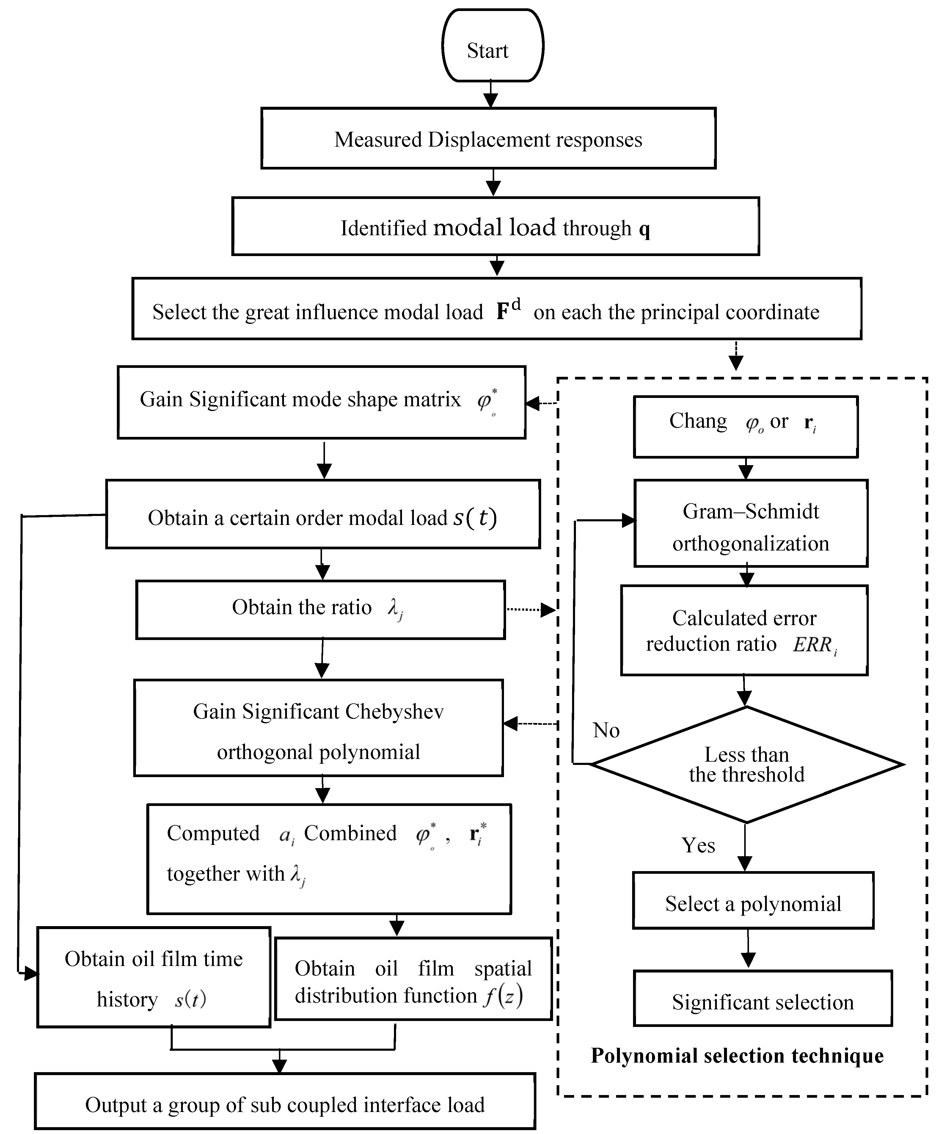
3. The Identification Processes of Sliding Bearing Coupling Interface Load

Generally speaking, the implementation details of sliding bearing coupling interface load identification combined POD decomposition algorithm with polynomial selection technique, described in Figure 2, can be summarized as follows:

Step 1: Combine the measured response together with the centralized dynamic load identification method to identify the modal load on the corresponding concentrated load node;

Step 2: Combine the modal load together with the blind source separation method to calculate the great influence of the modal load ${\mathbf{F}}^{\mathrm{d}}$ on each principal coordinate;

Step 3: Combine the great influence modal load ${\mathbf{F}}^{\mathrm{d}}$ with polynomial selection technique to denote a certain order modal load as the corresponding oil film time history;

Step 4: Calculate the ratio ${\mathsf{\lambda }}_j$ by comparing other order modal loads with a specific order modal load. Employ the polynomial structure selection technique based on the error reduction ratio of this ratio to select effective Chebyshev polynomials ${\mathbf{R}}_i$ and identify the corresponding coefficient $a_i$. This process yields a group of oil film spatial distribution functions;

Step 5: Apply the same method to identify other groups of oil film time history and the corresponding oil film spatial distribution function;

Step 6: Multiply the identified oil film time history and the corresponding oil film spatial distribution function to derive a group of sub-coupled interface loads. The linear superposition of the k sub-coupled interface load synthesizes the coupling interface load of the sliding bearing.

To explicitly evaluate the accuracy between the identified $\tilde{\mathit{F}}$ and the actual load F using this proposed method, the following evaluation metrics are defined: correlation coefficient function $\mathrm{CC}\left(\mathit{F},\tilde{\mathit{F}}\right)$.

$$\mathrm{CC}\left(\mathit{F},\tilde{\mathit{F}}\right)={\displaystyle \frac{\sum \sum \left[\mathit{F}-E\left(\mathit{F}\right)\right]\left[\tilde{\mathit{F}}-E\left(\tilde{\mathit{F}}\right)\right]}{‖\tilde{\mathit{F}}-E\left(\tilde{\mathit{F}}\right)‖‖\mathit{F}-E\left(\mathit{F}\right)‖}}$$

(12)

where $E\left(•\right)$ represents calculating the expected value of the corresponding matrix or vector. $\mathrm{RE}\left(\mathit{F},\tilde{\mathit{F}}\right)$ denotes the relative error function and $\mathit{RE}\left(\mathit{F},\tilde{\mathit{F}}\right)={\displaystyle \frac{‖\tilde{\mathit{F}}-\mathit{F}‖}{‖\mathit{F}‖}}$.

4. Numerical Example

The model of the wind turbine gearbox shaft system in this case study is illustrated in Figure 3a. The transfer matrix model shown in Figure 3b used to obtain the structural mass matrix, structural damping matrix, and structural stiffness matrix is constructed according to the transfer matrix method in the literature [30], which is subdivided into 18 elements consisting of 19 nodes. The material properties of the main shaft of the wind turbine gearbox are uniform, with an elastic modulus of 125 Gpa, a Poisson’s ratio of 0.335, and a density of 8850 kg/m³. According to the surrogate model construction method of wind power sliding bearing lubrication characteristics provided by the literature [31], it is assumed that the expression for the coupling interface load of the sliding bearing in the wind turbine gearbox is as follows $\mathit{F}\left(t,h(z)\right)=(400\sin \left(z^{2}t\right)+600\sin \left(z^1{t}^2\right)+1000\mathrm{s}\mathrm{i}\mathrm{n}(t^3))$, $t\in \left[0,2\right]s$, $z\in \left[0,0.2\right]\mathrm{m}$, acting vertically along the y direction on the left end area (0 ~ 200 mm) of the main shaft. The spatial distribution function is discretized into 101 points, and the oil film time history is discretized into 101 points.

4.1. The Sliding Bearing Coupling Interface Load Decomposed

Using the POD algorithm, the sliding bearing coupling interface load is decomposed into a linear combination of the sub-coupled interface load, which is independent in terms of oil film time history and spatial distribution, as shown in Figure 4. The sliding bearing coupling interface load is decomposed into three groups of sub-coupled interface load with oil film spatial distribution functions (shown in Figure 4a) and corresponding oil film time histories (shown in Figure 4b). The sub-coupled interface load corresponding to each group of oil film time history and spatial distribution functions are (shown in Figure 4c). The absolute error, as observed in Figure 4d, fluctuates between −100 N and 100 N, with an overall relative error of RE = 3.18 × 10⁻⁵, indicating a minimal discrepancy compared to the real sliding bearing coupling interface load. Hence, the sliding bearing coupling interface load in this study can be equivalently represented by three groups of the sub-coupled interface load. The sliding bearing coupling interface load identification can be transformed into three groups of sub-coupled interface load identification.

4.2. Obtain Displacement Response

The form of the main shaft transient displacement response is mainly determined by the multiple independent oil film time histories of the sliding bearing coupling interface load together, and the oil film spatial distribution functions are the factors that influence the transient displacement response amplitude. According to the modal transformation, the modal loads are the linear combination of the three groups of oil film time histories, and the amplitude coefficients are affected by the three groups of oil film spatial distribution functions. Via the blind source separation method, the modal load with great influence on each oil film time history function is obtained. As the blind source separation method has been investigated and widely used in the field of signal processing, the deductions and formulations of the basic functions are not provided here, which can refer to reference [6].

In this study, the main shaft transient displacement response used to identify modal load based on the centralized dynamic load identification method is obtained using three groups of the equivalent sub-coupled interface load of the five concentrated load points of nodes 1–5 shown in Figure 3b, three groups of the sub-coupled interface load shown in Figure 4c can be expressed as follows: Node 1 −0.0928×$s_1\left(t\right)$+ 0.1741×$s_2\left(t\right)$ − 0.1834×$s_3(t)$; Node 2 −0.1921×$s_1(t)$ + 0.1791× $s_2\left(t\right)$ + 0.0284×$s_3(t)$; Node3 −0.1988×$s_1(t)$ + 0.0073×$s_2\left(t\right)$ + 0.2198×$s_3(t)$; Node 4 −0.2056×$s_1(t)$ − 0.1636× $s_2(t)$ + 0.0843×$s_3(t)$; Node 5 −0.1062×$s_1\left(t\right)-$0.1651×$s_2\left(t\right)$ − 0.2454×$s_3(t)$. The transient displacement responses of the more sensitive nodes 6, 9, 12, 15, and 19 out of 19 nodes in the main shaft to the sub-coupled interface load are collected, as shown in Figure 5.

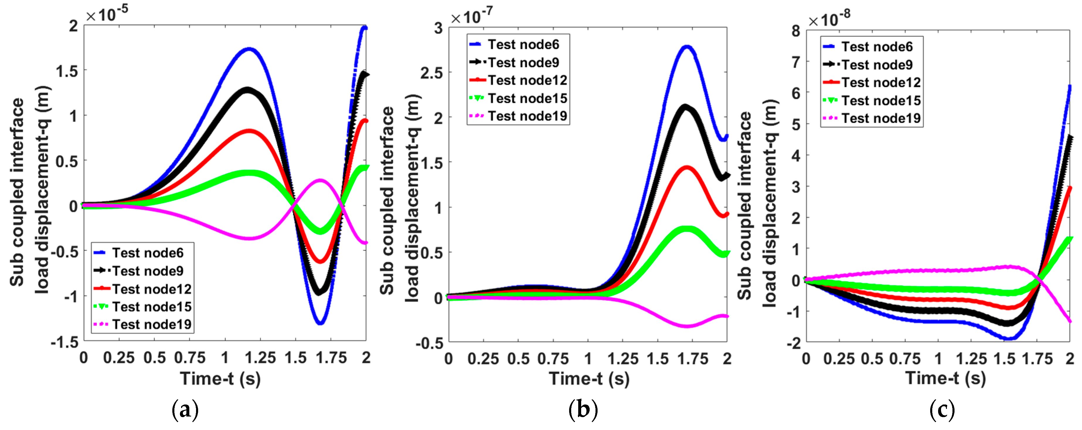
4.3. Result Discussion of Identify Sub-Coupled Interface Load

Based on the displacement response coming from the first group of the sub-coupled interface load, equivalent concentrated time-domain loads at load nodes 1, 2, 3, 4, and 5 are identified, as illustrated in Figure 6a. The wind turbine gearbox main shaft model is divided into 19 nodes with 76 modal orders, as shown in Figure 3b. Five effective modal orders, specifically the 16th, 23rd, 42nd, 54th, and 67th, are selected using the polynomial structure selection technique. A comparative analysis between the oil film time history of the first group of the sub-coupled interface load and the 16th modal load at the 5th load node reveals a difference only in amplitude, with C 4.1 being −821.3365, as shown in Figure 6b. This confirms that the oil film time history of the sub-coupled interface load and their modal loads share the same functional form, differing only in amplitude by a coefficient relationship. The ratio of the 16th, 23rd, 42nd, 54th, and 67th modal loads of the five load nodes to the 16th modal loads of the first load node is ${\lambda }_1=1$, ${\lambda }_2=-1.1280$, ${\lambda }_3=0.8409$, ${\lambda }_4=-2.8514$, and ${\lambda }_5=-25.2032$.

The six Chebyshev orthogonal polynomials described in Equation (13) are equivalent to the load point of 1–5 nodes of the wind turbine gearbox main shaft. The equivalent amplitude coefficient is shown in

Table 1. Evaluation indicators for identifying loads.

Load	$\mathbf{CC}\left(\mathit{F},\tilde{\mathit{F}}\right)$			$\mathbf{RE}\left(\mathit{F},\tilde{\mathit{F}}\right)$
	$\mathit{l}\left(\mathit{t}\right),\mathit{s}\left(\mathit{t}\right)/\mathit{c}2$	$\mathit{h}\left(\mathit{z}\right),\mathit{c}2\mathit{f}\left(\mathit{z}\right)$	$\mathit{F}\left(\mathit{t}\mathbf{,}\mathit{h}(\mathit{z})\right),\tilde{\mathit{F}}\left(\mathit{t}\mathbf{,}\mathit{h}(\mathit{z})\right)$	$\mathit{l}\left(\mathit{t}\right),\mathit{s}\left(\mathit{t}\right)/\mathit{c}2$	$\mathit{h}\left(\mathit{z}\right),\mathit{c}2\left(\mathit{z}\right)$	$\mathit{F}\left(\mathit{t}\mathbf{,}\mathit{h}(\mathit{z})\right),\tilde{\mathit{F}}\left(\mathit{t}\mathbf{,}\mathit{h}(\mathit{z})\right)$
The first group	0.9995	1	0.9995	2.83%	0.62%	2.99%
The second group	0.9998	1	0.9999	1.68%	0.61%	1.81%
The third group	0.9995	0.9951	0.9945	1.85%	10.92%	11.08%
Coupling interface load	—	—	0.9995	—	—	3.00%

. Utilizing the polynomial selection technique based

$$\left\{\begin{array}{l}{R}_{\mathbf{1}}\left(z\right)=\mathbf{1}\\ R_{\mathbf{2}}\left(z\right)=z\\ R_{\mathbf{3}}\left(z\right)=\mathbf{2}{z}^{\mathbf{2}}-\mathbf{1}\\ R_{\mathbf{4}}\left(z\right)=\mathbf{4}{z}^{\mathbf{3}}-\mathbf{3}z\\ R_{\mathbf{5}}\left(z\right)=8z^{\mathbf{4}}-8z^{\mathbf{2}}-1\\ R_{\mathbf{6}}\left(z\right)=16z^{\mathbf{5}}-20z^{\mathbf{3}}+5z\\ \cdots \end{array}\right.$$

(13)

on the error reduction ratio, the first and second terms of the six Chebyshev orthogonal polynomials are identified as effective from the ratio ${\lambda }_i$. The Chebyshev orthogonal polynomial coefficients $a_1=-81.6080,a_2=5.6587,a_3=0$, $a_4=0$, $a_5=0,$ and $a_6=0$ are identified according to Equation (10). These coefficients are then multiplied with the corresponding Chebyshev orthogonal polynomials to fit the oil film spatial distribution function of the first group of the sub-coupled interface load. A comparison with the actual oil film spatial distribution function, as shown in Figure 6c, reveals that the actual and fitted oil film spatial distribution functions of the first group of sub-coupled interface load differ only in amplitude, with the inverse of the amplitude also being −821.3365. A comparison of the identified and actual first group of sub-coupled interface load and their errors, as depicted in Figure 6f, indicates a minimal identification error and a high degree of conformity with the actual first set of the sub-coupled interface load. Evaluation metrics of the identified parameters compared to the original parameters are shown in the first row of Table 1.

The minimum correlation coefficient for the oil film time history of the first set sub-coupled interface load is 0.9995, the minimum correlation coefficient for the spatial distribution function is 1, and the minimum correlation coefficient for the sub-coupled interface load is 0.9995; the relative error for the oil film time history of the first set of the sub-coupled interface load is 2.83%, the relative error for the spatial distribution function is 0.62%, and the maximum overall relative error is 2.99%.

Based on the displacement response of the second group of the sub-coupled interface load, equivalent concentrated time-domain loads at the five load nodes mentioned above are identified, as shown in Figure 7a. Five effective modal orders, namely the 10th, 14th, 23rd, 28th, and 56th, are selected for these five equivalent concentrated time-domain loads using the polynomial structure selection technique. As illustrated in Figure 7b, a comparative analysis between the oil film time history of the actual second group of the sub-coupled interface load and the 10th modal load at the first load node shows that they share the same functional form, differing only in amplitude by a coefficient, denoted as C. The ratio of the 10th, 14th, 23rd, 28th, and 56th modal loads at the five load nodes to the 10th modal load at the first node are ${\lambda }_1=1$, ${\lambda }_2=-0.5473$, ${\lambda }_3=-1.4656$, ${\lambda }_4=0.0490,$ and ${\lambda }_5=-0.7377$, respectively. Employing the polynomial structure selection technique based on the error reduction ratio and the ratio ${\lambda }_i$, the first and second terms are identified as effective from the six Chebyshev orthogonal polynomials. The coefficients $a_1=-0.2177$, $a_2=9.8711$, $a_3=0$, $a_4=0$, $a_5=0,$ and $a_6=0$ of the Chebyshev orthogonal polynomials are identified. By multiplying these coefficients with the corresponding Chebyshev orthogonal polynomials, the oil film spatial distribution function of the second set of sub-coupled interface load is fitted and compared with the actual oil film spatial distribution function, as shown in Figure 7c. It is observed that the actual and fitted oil film spatial distribution functions of the second group of sub-coupled interface load differ only in amplitude, with the inverse of the amplitude being −57.8713. A comparative analysis between the identified and actual second group of the sub-coupled interface load and their errors, as depicted in Figure 7f, indicates minimal identification error and excellent conformity with the actual second set. The evaluation metrics of the identified parameters compared to the original parameters are presented in the second row of Table 1.

The minimum correlation coefficient for the oil film time history of the second group of sub-coupled interface load is 0.9998, for the oil film spatial distribution function is 1, and for the sub-coupled interface load is 0.9999; the relative error for the oil film time history of the second group of sub-coupled interface load is 1.68%, for the oil film spatial distribution function is 0.61%, and the maximum overall relative error is 1.81%.

Based on the displacement response of the third group of the sub-coupled interface load, equivalent concentrated time-domain loads at the five load nodes mentioned above are identified, as depicted in Figure 8a. Five effective modal orders, specifically the 10th, 14th, 23rd, 28th, and 56th, are selected for these five equivalent concentrated time-domain loads using the polynomial structure selection technique. A comparative analysis between the oil film time history of the actual third group of the sub-coupled interface load and the 10th modal load at the first load node is conducted, as shown in Figure 8b. Both demonstrate the same functional form and differ only in amplitude by a coefficient denoted as C. The ratios of the 10th, 14th, 23rd, 28th, and 56th modal loads at the five load nodes to the 10th modal load at the first node are ${\lambda }_1=1$, ${\lambda }_2=-2.8569$, ${\lambda }_3=0.7663$, ${\lambda }_4=-0.3558,$ and ${\lambda }_5=0.8836$, respectively. Utilizing the polynomial structure selection technique based on the error reduction ratio and the ratio λ, the first and second terms are identified as effective from the six Chebyshev orthogonal polynomials. The coefficients $a_1=7.5683$, $a_2=0$, $a_3=26.2981$, $a_4=1.4765$, $a_5=0,$ and $a_6=0$ of the Chebyshev orthogonal polynomials are identified. These coefficients are then multiplied with the corresponding Chebyshev orthogonal polynomials to fit the oil film spatial distribution function of the third group of sub-coupled interface load. A comparison with the actual oil film spatial distribution function of the third group, as shown in Figure 8c, reveals that the actual and fitted oil film spatial distribution functions differ only in amplitude, with the inverse of the amplitude being −161.7890. A comparative analysis of the identified and actual third set of the sub-coupled interface load and their errors, as depicted in Figure 8f, indicates a minimal identification error and excellent conformity with the actual third group. The evaluation metrics of the identified parameters compared to the original parameters are presented in the third row of Table 1. The minimum correlation coefficient for the oil film time history of the third group is 0.9995, for the oil film spatial distribution function is 0.9951, and for the sub-coupled interface load is 0.9945; the relative error for the oil film time history of the third group is 1.85%, for the oil film spatial distribution function is 10.92%, and the maximum overall relative error is 11.08%.

4.4. Identification of Sliding Bearing Coupling Interface Load

The sliding bearing coupling interface load is obtained by linearly superimposing the three groups of identified sub-coupled interface load, and its accuracy is compared with the actual sliding bearing coupling interface load and the corresponding errors, as shown in Figure 9. Overall, the identification error is minimal, and the linearly superimposed sliding bearing coupling interface load from the identified three groups of the sub-coupled interface load shows excellent agreement with the actual load. The evaluation metrics of the identified parameters compared to the original parameters are presented in the fourth row of Table 1. The minimum correlation coefficient for the sliding bearing coupling interface load is 0.9995, with a maximum relative error of 3.00%. These results demonstrate the accuracy of the improved identification method.

4.5. The Influence of Polynomial Selection Technique on Recognition Results

In order to verify the influence of the selection of effective modal vector and Chebyshev orthogonal polynomial terms on the accuracy of sliding bearing coupling interface load identification, the following three forms are compared and analyzed: (I) no choice; (II) only effective modal vectors are selected; (III) only the effective Chebyshev polynomials are selected. The recognition results of the three cases are shown in Figure 10. It can be seen from Figure 10 that the maximum overall relative error of (I) is 84.15 %; the maximum overall relative error of (II) is 63.87%. The maximum overall relative error of (III) is 18.65%. By comparing (II) and (III) with (I), it can be seen that the recognition accuracy of the oil film spatial distribution function and the oil film time history is improved, respectively. Among them, the recognition error of (II) is larger than that of (III). It can be concluded that the polynomial structure selection technology has a better effect on the oil film spatial distribution function than the time history recognition accuracy. At the same time, the identification method of selecting the effective mode and Chebyshev polynomial is more accurate than that of only one choice. It has been proved that the polynomial structure selection technology can improve the identification accuracy of the oil film time history and spatial distribution function of the sliding bearing coupled interface load obviously.

5. Conclusions

This paper analyzes the coupling interface load of sliding bearings in a wind turbine gearbox, which is a time and space coupled distribution load. The POD decomposition can transform the coupling interface into a linear superposition of space–time independent distributed loads. Therefore, a space–time independent distributed load identification method can be used to gain the sliding bearing coupling interface load, which is difficult to measure and calculate directly, and the introduction of polynomial selection can effectively improve the identification accuracy. The minimum correlation coefficient is 0.9995, and the overall maximum relative error is 3.00%. The results prove the accuracy and effectiveness of the identification and realize the effective identification of this complex coupled interface load. The main novelties of this improved method are as follows: (1) it deeply explores the multi-solution nature of sliding bearing coupling interface load identification, and the polynomial selection technique is used to deal with the recognition accuracy problem caused by this multi-solution nature; (2) it describes and identifies the sliding bearing coupling interface load from the viewpoint of the whole oil film time-domain and space-domain. Also, there are two main shortcomings of this improved method: one is to apply the sliding bearing coupling interface load to the main shaft as an external force rather than a conventional support force, and the other is that the displacement response does not take into account the fluctuations caused by other factors in engineering practice.

References

1. Fei, W.J.; Tan, J.J.; Li, H.; Zhu, C.C.; Sun, Z.D.; Wang, H.X. Influences of planet gear journal bearing on dynamic characteristics of megawatt-scale wind turbine drivetrains: Simulations and experiments. Mech. Syst. Signal Process. 2024, 221, 111747. [Google Scholar] [CrossRef]
2. Thomas, D.; Georg, J.; Carsten, G.; Julian, R.; Mattheüs, L.; Benjamin, L. Multiscale-simulation method for the wear behaviour of planetary journal bearings in wind turbine gearboxes. J. Phys. Conf. Ser. 2024, 2767, 052012. [Google Scholar]
3. Zhang, K.; Chen, Q.; Zhang, Y.B.; Zhu, J.; Wang, M.X.; Feng, K. Numerical and experimental investigations on thermoelastic hydrodynamic performance of planetary gear sliding bearings in wind turbine gearboxes. Tribol. Int. 2024, 191, 109081. [Google Scholar] [CrossRef]
4. Ding, H.; Mermertas, Ü.; Hagemann, T.; Schwarze, H. Calculation and Validation of Planet Gear Sliding Bearings for a Three-Stage Wind Turbine Gearbox. Lubricants 2024, 12, 95. [Google Scholar] [CrossRef]
5. Liu, Y.; Wang, L.; Li, M.; Wu, Z.M. A distributed dynamic load identification method based on the hierarchical-clustering-oriented radial basis function framework using acceleration signals under convex-fuzzy hybrid uncertainties Mechanical Syst. Signal Process. 2022, 172, 108935. [Google Scholar] [CrossRef]
6. Liu, J.; Li, K. Sparse identification of time-space coupled distributed dynamic load. Mech. Syst. Signal Process. 2021, 148, 107177. [Google Scholar] [CrossRef]
7. Li, K.L.; Xiao, L.F.; Liu, M.Y.; Kou, Y.F. A distributed dynamic load identification approach for thin plates based on inverse Finite Element Method and radial basis function fitting via strain response. Eng. Struct. 2025, 322, 119072. [Google Scholar] [CrossRef]
8. Bu, W.P.; Zhao, Y.M.; Shen, C. Fast and efficient finite difference/finite element method for the two-dimensional multi-term time-space fractional Bloch-Torrey equation. Appl. Comput. Math. 2021, 398, 125985. [Google Scholar] [CrossRef]
9. Huang, J.; Wang, F.; Qiao, L.; Yang, X. T-distributed stochastic neighbor embedding echo state network with state matrix dimensionality reduction for time series prediction. Eng. Appl. Artif. Intell. 2023, 122, 106055. [Google Scholar] [CrossRef]
10. You, Y.; Zhang, W.; Yan, Q.; Xu, J.; Wang, C.; Li, Z.; Su, H. Blade Failure Fault Reproduction Based on High Low Cycle Composite Fatigue Test Technology. Propuls. Technol. 2020, 41, 1130–1137. [Google Scholar]
11. Chen, D.Y.; Xiao, Q.; Sun, S.G. Method for identifying dynamic loads on strongly coupled structures. J. Mech. Eng. 2021, 57, 174–181. [Google Scholar]
12. Li, J.J.; Ren, Z.S.; Wu, Y.M.; Wang, Y.W. Method and experimental verification of load decoupling and dimensionality reduction calibration for high-speed train frames. J. Cent. South Univ. (Nat. Sci. Ed.) 2022, 53, 1730–1739. [Google Scholar]
13. Sun, X.G.; Guo, Y.C.; Nie, X.H. Research on Decoupling Method for Complex Load on Airframe Wall Panels. Eng. Test. 2023, 63, 4–6. [Google Scholar]
14. Cao, Z.K.; Sun, C.B.; Cui, M.; Zhou, L.; Liu, K. A fast methodology for identifying thermal parameters based on improved POD and particle swarm optimization and its applications. Eng. Anal. Bound. Elem. 2024, 169, 106001. [Google Scholar] [CrossRef]
15. Kawaguchi, M.; Lwasaki, M.; Nakayama, R.; Yamamoto, R.; Nakashima, A.; Ogato, Y. Mode analysis for multiple parameter conditions of nozzle internal unsteady flow using Parametric Global Proper Orthogonal Decomposition. Fluid Dyn. Res. 2024, 56, 055501. [Google Scholar] [CrossRef]
16. Chen, R.; Min, G.Y.; Hu, M.M.; Yang, S.G.; Cai, M.Q. Proper orthogonal decomposition (POD) dimensionality reduction combined with machine learning to predict the vibration characteristics of stay cables at different lengths. Measurement 2025, 242, 115827. [Google Scholar] [CrossRef]
17. Zhao, Y.; Li, Y.; Song, X. PIV Measurement and Proper Orthogonal Decomposition Analysis of Annular Gap Flow of a Hydraulic Machine. Machines 2022, 10, 645. [Google Scholar] [CrossRef]
18. Li, Z.L.; Niu, Y.P. Application of Orthogonal Polynomial Fitting Method to Extract Gravity Wave Signals from AIRS Data Related to Typhoon Deep Convection. Earth Space Sci. 2022, 9, e2022EA002408. [Google Scholar] [CrossRef]
19. Wang, J.; Li, X.; Wang, Z.; Davey, P.G.; Li, Y.; Yang, L.; Lin, M.; Zheng, X.; Bao, F.; Elsheikh, A. Accuracy and reliability of orthogonal polynomials in representing corneal topography. Med. Nov. Technol. Devices 2022, 15, 100133. [Google Scholar] [CrossRef]
20. Li, K.; Liu, J.; Han, X.; Sun, X.; Jiang, C. A novel approach for distributed dynamic load reconstruction by space-time domain decoupling. J. Sound Vib. 2015, 348, 137–148. [Google Scholar] [CrossRef]
21. Li, K.; Liu, J.; Han, X.; Jiang, C.; Zhang, D. Distributed dynamic load identification based on shape function method and polynomial selection technique. Inverse Probl. Sci. Eng. 2016, 25, 1323–1342. [Google Scholar] [CrossRef]
22. Luo, S.; Jiang, J.; Zhang, F.; Mohamed, M.S. Distributed Dynamic Load Identification of Beam Structures Using a Bayesian Method. Appl. Sci. 2023, 13, 2537. [Google Scholar] [CrossRef]
23. Liu, J.; Sun, X.S.; Han, X.; Jiang, C.; Yu, D.J. Dynamic load identification for stochastic structures based on Gegenbauer polynomial approximation and regularization method. Mech. Syst. Signal Process. 2014, 56–57, 35–54. [Google Scholar] [CrossRef]
24. Sanchez, J.; Benaroya, H. Review of force reconstruction techniques. J. Sound Vib. 2014, 333, 2999–3018. [Google Scholar] [CrossRef]
25. Lu, C.; Liu, J.; Jiang, C. Research on nonlinear model identification of the hydragas suspension based on structure-selection techniques. Mech. Sci. Technol. Aerosp. Eng. 2014, 33, 1293–1297. [Google Scholar]
26. He, H.; Jing, J. Modified oil film force model for investigating motion characteristics of rotor-bearing system. J. Vib. Control. 2016, 22, 756–768. [Google Scholar] [CrossRef]
27. Geng, Y.; Zhu, K.D.; Qi, S.M.; Liu, Y.; Yu, R.F.; Chen, W.; Liu, H. A deterministic mixed lubrication model for parallel rough surfaces considering wear evolution. Tribol. Int. 2024, 194, 109443. [Google Scholar] [CrossRef]
28. Rodriguez, P.C.; Marti-Puig, P.; Caiafa, C.F.; Serra-Serra, M.; Cusidó, J.; Solé-Casals, J. Exploratory Analysis of SCADA Data from Wind Turbines Using the K-Means Clustering Algorithm for Predictive Maintenance Purposes. Machines 2023, 11, 270. [Google Scholar] [CrossRef]
29. Mao, W.; Pei, S.; Guo, J.; Li, J.; Wang, B. An Electromagnetic Load Identification Method Based on the Polynomial Structure Selection Technique. Shock. Vib. 2024, 2024, 1842508. [Google Scholar] [CrossRef]
30. Mao, W.; Han, X.; Liu, G.; Liu, J. Bearing dynamic parameters identification of a flexible rotor-bearing system based on transfer matrix method. Inverse Probl. Sci. Eng. 2015, 24, 372–392. [Google Scholar] [CrossRef]
31. Li, J.H.; Mao, W.G.; Feng, D. Lubrication characteristic surrogate model construction of wind power sliding bearing based on Polynomial structure selection technology. Lubr. Eng. 2023, 48, 173–181. [Google Scholar]
Figure 1. Geometrical model and coordinate system from the literature [3].
Machines 12 00848 g001
Figure 2. Identification flow chart.
Machines 12 00848 g002
Figure 3. Sliding bearing structure of wind turbine gearbox.
Machines 12 00848 g003
Figure 4. POD decomposition of the coupled interface load of sliding bearings. (a) Three groups of oil film spatial distribution functions (b) Three groups of oil film time histories. (c) Three groups of sub-coupled interface load. (d) Real and linearly superimposed coupling interface load and error.
Machines 12 00848 g004
Figure 5. Displacement response under three groups of the sub-coupled interface load. (a) Group 1; (b) Group 2; (c) Group 3.
Machines 12 00848 g005
Figure 6. Identification of the first group of the sub-coupled interface load based on polynomial structure selection technology. (a) Equivalent concentrated time load. (b) The oil film time history. (c) The oil film spatial distribution function. (d) Real sub-coupled interface load. (e) Identification of sub-coupled interface load. (f) Identification error.
Machines 12 00848 g006
Figure 7. Identification of the second group of the sub-coupled interface load based on polynomial structure selection technology. (a) Equivalent concentrated time load. (b) The oil film time history. (c) The oil film spatial distribution function. (d) Real load. (e) Identification load. (f) Identification error.
Machines 12 00848 g007
Figure 8. Identification of the third group of the sub-coupled interface load based on polynomial structure selection technology. (a) Equivalent concentrated time load. (b) The oil film time history. (c) The oil film spatial distribution function. (d) Real load (e) Identification load (f) Identification error.
Machines 12 00848 g008
Figure 9. Identification of coupled interface load of sliding bearings under polynomial structure selection technique. (a) The coupled interface load. (b) Linear superposition of three groups of loads. (c) Identification error.
Machines 12 00848 g009
Figure 10. Comparison of errors in load identification under different selection scenarios.
Machines 12 00848 g010aMachines 12 00848 g010b