An Extend Sliding Mode Disturbance Observer for Optical Inertial Platform Line-of–Sight Stabilized Control

Abstract

As the imaging distance and focal length of photoelectric systems increase, the requirements for line-of–sight stabilization of optical inertial stabilized platforms (ISPs) become higher. Disturbance rejection directly determines the stability accuracy of optical inertial stabilized platforms. However, the accurate observation and suppression of wide-band and rapidly changing disturbances remains a challenge in current engineering applications. This paper proposes a robust extended sliding mode observer (ESMO) method to improve disturbance estimation performance. First, the linear extended state observer (LESO) is designed by taking the total disturbances as extended states. Then, a sliding mode observer (SMO) is incorporated in the extended states of the extended observer, forming a robust ESMO. Subsequently, the robustness and convergence characteristics of the proposed method are mathematically proved, revealing that it operates robustly without knowing the disturbance’s upper bound and offers faster dynamics and higher accuracy than the LESO. Finally, a series of simulation experimental tests are performed to demonstrate the effectiveness of the proposed method. The proposed method observes wide-band and rapidly changing disturbances utilizing the rapidly switching characteristic of the SMO and smooths the jitter of the SMO by cascading sliding mode estimation to the differentiation term of extended observation, achieving the integral effect of the reaching law. Meanwhile, this method only requires adjusting two parameters, making it suitable for engineering applications. It can be effectively used in optical inertial stabilized platform control systems for disturbance estimation and compensation.

1. Introduction

High precision stability is the core issue of ISP control. The motion of sensing instruments, such as cameras and lasers mounted on a platform, should be isolated from base disturbances. ISPs usually use the inner loop to reject external disturbances as the stabilization loop [1,2]. Especially with the increase in sensing instruments’ distance and the lengthening of focal length, the demand for stable control of optical ISP is becoming higher.

The overall stability performance mainly depends on the inner loop’s ability to reject external disturbances, and the most critical performance metric for an ISP is torque disturbance rejection [3,4]. The disturbance suppression performance of the ISP, determining the stability accuracy, is key to achieving high-precision stability, especially the suppression effect of rapidly changing disturbances. Disturbance suppression is gradually classified into two methods. One method achieves disturbance compensation through measuring disturbances, which requires additional disturbance measurement sensors, and another method uses disturbance observers. For some disturbance signals that cannot be directly obtained through sensors, disturbance observer methods are becoming increasingly popular. Various methods of disturbance observers achieving satisfactory effects have been proposed. The extended state observer (ESO) concept proposed by Han [5] is a famous and effective method used to achieve robust control. This method can estimate and compensate for total disturbances and is independent of the object model (unmodeled dynamics and unknown disturbances), showing immense potential for solving control problems.

The linear extended state observer (LESO) and nonlinear extended state observer (NESO) have been adopted in active disturbance rejection control (ADRC) to compensate for uncertainties, successfully applied to several applications. Ahi et al. applied ADRC to a one-axis gimbal mechanism, illustrating its effectiveness against external disturbances and parameter uncertainties [6]. Yao et al. proposed an ESO via the backstepping method to track control of a class of uncertain parametric and uncertain nonlinearities, demonstrating its tracking performance in a robot manipulator [7]. Wang et al. proposed an enhanced linear active disturbance rejection control (LADRC) in the sensor-less control of an interior permanent magnet synchronous motor (IPMSM). The LADRC with cascaded ESO guaranteed relatively timely and accurate estimation of the total disturbance [8]. Yuan et al. designed an NESO adopted in ADRC to control the pneumatic muscle actuator system, demonstrating its effectiveness under various sampling intervals and disturbances [9]. Rsetam et al. studied a new cascaded ESO-based sliding mode control (SMC) for an underactuated flexible joint robot. The cascaded ESO estimated the uncertain disturbances, verifying its performance in dealing with control challenges including coupling, underactuation, nonlinearity, uncertainties, external disturbances, and noise amplification [10]. The ADRC with ESO applied to the current control, speed control, and position control of permanent magnet synchronous motors was fully reviewed [11]. Yan et al. proposed an enhanced nonlinear ADRC scheme that integrated a cascaded ESO to achieve timely and accurate disturbance estimations, improving speed control performance of the generator rotor characterized by resistance to load shocks [12]. Chen et al. proposed a nonlinear extended state observer and recursive sliding mode control [13]. The extended state observer observes lumped disturbances including load variations, wind gusts, and inaccurate model parameters in quadrotor dynamics. The recursive sliding mode controller scheme reduced chattering and ensured fast response.

From these studies, the NESO observed by nonlinear state feedback makes implementation somewhat difficult [14]. For the conventional LESO, the estimated disturbance performance has been proven. The estimated disturbance can be regarded as the true disturbance filtered by a typical second-order low pass filter, and the steady-state tracking error of the speed control system is proportional to the first derivative of the total disturbance [15]. Therefore, the LESO with a larger bandwidth is proposed to reject time-varying disturbances. However, as mentioned, the adoption of a high-gain LESO increases noise sensitivity [16]. Although the LESO is easy to implement and effective against low-frequency, slow-moving disturbances, it has difficulty suppressing wide-band and rapidly changing interference. The LESO cannot balance the estimation accuracy and speed, resulting in a steady-state estimation error.

In actual optical ISPs, there are numerous nonlinear and rapidly changing disturbances from both external and internal sources. External disturbance sources for the aircraft include attitude changes of the base, gusts, vibration disturbances, and micro-vibration disturbances. Internal sources involve nonlinear sudden changes in the friction torque of the ISP’s internal shaft system, cable twisting torque fluctuations, and torque ripple caused by the motor’s cogging effect. These external and internal disturbances exhibit wide-band and rapidly changes.

Sliding mode control is a well-known nonlinear control method with strong robustness and fast response due to its sign function, which directly controls based on the polarity of the error. Many studies have proven that the sliding mode technique in observers is able to achieve high-performance and satisfactory control effects in systems with nonlinear characteristics or rapidly changing disturbances. When the system is on the sliding mode surface, its responses and states remain insensitive to both parameter perturbation and external disturbances. Rsetam et al. proposed terminal sliding mode control and a cascaded finite-time sliding mode observer for high-order underactuated flexible joint robot trajectory tracking, achieving robustness against lumped disturbance and estimation error [17]. Neisarian et al. proposed a novel fast finite-time velocity observer-based terminal sliding mode controller for nonlinear systems in the presence of unknown time-varying matched uncertainties and input saturation constraints [18]. Zhu et al. proposed an adaptive sliding mode disturbance observer (SMO) to compensate for free-flying space manipulator system with complex and uncertain dynamics after capturing a space target with uncertain mass [19]. Lu designed a sliding mode disturbance observer with switching-gain adaptation based on the internal model principle for a class of nonlinear systems, alleviating the chattering problem [20]. Deng et al. designed a hybrid control strategy combining adaptive sliding mode control and SMO to improve the performance of the permanent magnet synchronous motor current loop, restraining external disturbances and reducing sliding mode control gains [21]. Rabiee proposed an adaptive SMO for finite-time disturbance estimation, relaxing assumptions on disturbances and ensuring convergence of the disturbance observer error to the origin in finite time [22]. A robust SMO was designed to improve disturbance rejection performance of the photoelectric stabilized platform, with friction torque and moving base disturbances observed to compensate by feedback and feedforward [23]. A continuous global sliding mode controller equipped with a nonlinear disturbance observer was designed to effectively address various challenges including uncertainties, disturbances, unmodeled dynamics, and unmodeled frictions. This controller also effectively resolves chattering issues and demonstrates strong regulation and disturbance estimation performance [24]. A sliding mode–assisted observer with an adaptive law was designed to estimate the residual-disturbance estimation error of the disturbance observer to suppress rapidly changing disturbances [25]. Chen et al. proposed an adaptive sliding mode disturbance observer-based finite-time control scheme with prescribed performance in an unmanned aerial manipulator system. The observer with a nested adaptive structure estimated and compensated for external disturbances and state-dependent uncertainties in finite time [26].

These SMDOs achieve some effect; however, the use of the sign function, while crucial for addressing nonlinear characteristics and rapidly changing disturbances, also introduces chattering in sliding mode techniques. It should be pointed out that in an independent SMDO system, the upper bound of the total lumped disturbance and uncertainties needs to be known, and the sliding mode gain must be greater than it, which is difficult to acquire in practical systems [25]. The SMO based on terminal sliding mode technique may converge slowly when the initial state is far from the equilibrium region. Additionally, this approach requires solving a singular problem within the state observer. In contrast, the SMO system that utilizes gain-adaptive adjustment experiences constant changes in sliding mode gain, leading to decreased observation accuracy during the gain-switching process. Furthermore, these SMO systems contain multiple parameters that influence estimation accuracy and require careful adjustment. The suitable selection of these parameters is difficult and requires a thorough understanding of the controlled object.

To solve the problem of estimating wide-band and rapidly changing disturbances caused by some nonlinear factors, an ESMO method is proposed in this paper.

The main contributions of this paper are as follows:

(1) The proposed ESMO utilizes the bang-bang switching characteristic of the sliding mode to compensate for the LESO’s deficiency in observing rapidly changing disturbances. The proposed method smooths the jitter of the SMO by cascading sliding mode estimation to the differentiation term of extended observation, achieving the integral effect of the reaching law. At the same time, chattering is considered part of the ‘total disturbance’, which is observed by the LESO to achieve fast and accurate estimation.

(2) The stability and convergence characteristics of the proposed method are mathematically proved, revealing that it operates stably without knowing the disturbance’s upper bound and offers faster dynamics and higher accuracy than the LESO.

(3) The proposed ESMO presents a general observer scheme, demonstrating that various forms of extended sliding mode observers can be obtained by combining the ESO with other forms of sliding mode observers.

The remainder of this paper is organized as follows. Section 2 describes the problem investigated in this study. Section 3 introduces the proposed method. Section 4 analyzes the stability and convergence characteristics of the proposed method. Section 5 presents the simulation experimental results. Finally, Section 6 concludes the paper.

2. Line-of-Sight Stabilization Control Problem of Optical Inertial Platforms

Generally, the inertial stabilization platform is driven by a DC motor. Without loss of generality, its motion model is as follows shown in Equation (1):

$$J\dot{\omega }(\mathrm{t})=C_{m}i(t)+B\omega (t)+\Delta T_d$$

(1)

where J is the equivalent rotational inertia of the motor shaft, ${∆T}_d$ is the disturbance torque referred to the motor shaft, $\omega \left(t\right)$ is the angular velocity of optical inertial platform, $C_m$ is the torque constant of the motor, B is the friction coefficient, and $i\left(t\right)$ is the control current of the motor.

In practice, J and $C_m$ are time-varying parameters, which vary with temperature, air pressure, and other factors. The friction coefficient B is also difficult to determine accurately. Therefore, in control system design, nominal values $J_n$ and $C_{mn}$ are typically used for J and $C_m$ respectively. The deviations between the true values are denoted as $∆J$ and $∆C_m$. Thus, Equation (1) can be expressed as

$$\left(J_n+\Delta J\right)\dot{\omega }(t)=\left(C_{mn}+\Delta C_m\right)i(t)+B\omega (t)+\Delta T_d$$

(2)

From Equation (2), we can obtain

$$\dot{\omega }(t)={\displaystyle \frac{C_{mn}i(t)}{J_n}}+{\displaystyle \frac{B\omega (t)+\Delta T_d-\Delta J\dot{\omega }(t)+\Delta C_{m}I}{J_n}}$$

(3)

Let

$$d\left(t\right)={\displaystyle \frac{B\omega +\Delta T_d-\Delta J\dot{\omega }+\Delta C_{m}I}{J_n}}$$

(4)

And d(t) can be considered as total disturbance. Then the system model can be expressed as Equation (5)

$$\dot{\omega }(t)={\displaystyle \frac{C_{mn}i(t)}{J_n}}+d\left(t\right)$$

(5)

It can be seen that the system disturbance d(t) consists of multiple components, including disturbances caused by time-varying parameters, frictional damping, and external uncertainties. Therefore, the disturbance d(t) is nonlinear and rapidly changing. If d(t) can be accurately estimated, the total disturbance can be precisely compensated.

3. Design of the Extended Sliding Mode Observer

Let the state variable $X(t)=\left[\begin{array}{c}{x}_1\left(t\right)\\ x_2\left(t\right)\end{array}\right]=\left[\begin{array}{c}\omega \left(t\right)\\ d\left(t\right)\end{array}\right]$ and the input variable $u\left(t\right)=i\left(t\right)$. Then, the extended state equation of $d\left(t\right)$ can be shown as Equation (6)

$$\left\{\begin{array}{l}{\dot{x}}_1\left(t\right)=x_2\left(t\right)+{\displaystyle \frac{c_{mn}}{J_n}}u\left(t\right)\hfill \\ {\dot{x}}_2\left(t\right)=\dot{d}\left(t\right)\hfill \end{array}\right.$$

(6)

Assuming the upper bound of the disturbance derivative is p as shown in Equation (7), with the inertial stabilized platform current u(t) = i(t) and angular velocity ω(t) as inputs, and the observed state variable set as $\widehat{x}(t)=\left[\begin{array}{c}{\widehat{x}}_1\left(t\right)\\ {\widehat{x}}_2\left(t\right)\end{array}\right]$, the disturbance d(t) is observed as a new state. ${\widehat{x}}_1\left(t\right)$ is the estimate of the rotational speed ω(t), and ${\widehat{x}}_2\left(t\right)$ is the estimate of the disturbance d(t). The differential of d(t) is bounded, and the upper bound is less than p

$$\left|\dot{d}\left(t\right)\right|<p$$

(7)

The LESO is established as shown in Equation (8)

$$\left\{\begin{array}{l}{\dot{\widehat{x}}}_1\left(t\right)={\widehat{x}}_2\left(t\right)+{\beta }_1[x_1\left(t\right)-{\widehat{x}}_1\left(t\right)]+{\displaystyle \frac{c_{mn}}{J_n}}u\left(t\right)\hfill \\ {\dot{\widehat{x}}}_2\left(t\right)={\beta }_2[x_1\left(t\right)-{\widehat{x}}_1\left(t\right)]\hfill \end{array}\right.$$

(8)

A parameterized design method based on the bandwidth concept is used to determine the parameters of the LESO [27,28], with ${\beta }_1=2{\omega }_o$ and ${\beta }_2={\omega }_o^2$, where ${\omega }_o$ is the bandwidth of the extended state observer. The LESO performs well for low-frequency and slowly varying disturbances but poorly for rapidly changing disturbances. To compensate for rapidly changing disturbances, a sliding mode observer is cascaded to the LESO. The sliding mode control input $u_{smo}\left(t\right)$ is added to the control u(t), utilizing the switching characteristics of sliding mode to enhance the observation of rapidly changing disturbances. The ESMO is designed as follows:

$$\left\{\begin{array}{l}{\dot{\widehat{x}}}_1\left(t\right)={\widehat{x}}_2\left(t\right)+{\beta }_1\left[x_1\left(t\right)-{\widehat{x}}_1\left(t\right)\right]+{\displaystyle \frac{c_{mn}}{J_n}}u\left(t\right)\hfill \\ {\dot{\widehat{x}}}_2\left(t\right)={\beta }_2\left[x_1\left(t\right)-{\widehat{x}}_1\left(t\right)\right]+u_{smo}\left(t\right)\hfill \end{array}\right.$$

(9)

Comparing the first row of the ESMO in Equation (9) with the first row of the system model in Equation (6), it can be seen that the observation of the total disturbance d(t), denoted as $\widehat{d}(t)$, is the sum of the observations from the extended observer and the sliding mode observer, that is

$$\widehat{d}\left(t\right)={\widehat{x}}_2\left(t\right)+u_{smo}\left(t\right)$$

(10)

We define the observation error of the ESMO shown in Equation (9) as

$$e_{\omega }\left(t\right)=e_1\left(t\right)=\omega \left(t\right)-{\widehat{x}}_1\left(t\right)=x_1\left(t\right)-{\widehat{x}}_1\left(t\right)$$

(11)

$$e_d\left(t\right)=d\left(t\right)-\widehat{d}\left(t\right)=x_2\left(t\right)-{\widehat{x}}_2\left(t\right)= e_2(t)$$

(12)

where $e_{\omega }\left(t\right)$ and $e_1\left(t\right)$ are the observation errors of ω(t), $e_d\left(t\right)$ and $e_2(t)$ are the observation errors of $d\left(t\right)$.

Setting the sliding mode surface $\sigma \left(t\right)$ as

$$\sigma \left(t\right)={\dot{e}}_1\left(t\right)+{\beta }_1{e}_1\left(t\right)$$

(13)

In order to guarantee that the state variables always stay on the sliding manifold σ(t), reaching law $u_{smo}\left(t\right)$ is designed as follows:

$$u_{smo}\left(t\right)={{\displaystyle \int }}_0^{t}qsgn\left[\sigma \left(t\right)\right]dt$$

(14)

where q > 0 is the switching gain and sgn( ) is the switching function, which is

$$sgn\left[\sigma \left(t\right)\right]=\left\{\begin{array}{c}1 \sigma \left(t\right)>0\\ 0 \sigma \left(t\right)=0\\ -1 \sigma \left(t\right)<0\end{array}\right.$$

(15)

By organizing Equations (9)–(15), the sliding mode observer $u_{smo}\left(t\right)$ shown in Equation (14) is incorporated in the extended states in Equation (9), forming a robust ESMO shown in Equation (16). The ESMO observes wide-band and rapidly changing disturbances utilizing the rapidly switching characteristic of the SMO shown in Equation (14) and smooths the jitter of the SMO by cascading sliding mode estimation to the differentiation term of extended observation, achieving the integral effect of the reaching law. The extended sliding mode observer for the system in Equation (6) can be obtained as Equation (16), where ${\widehat{x}}_1\left(t\right)$ is the estimate of $x_1\left(t\right)$, and ${\widehat{d}\left(t\right)=\widehat{x}}_2\left(t\right){+u}_{smo}\left(t\right)$ is the estimate of $d\left(t\right)$

$$\left\{\begin{array}{l}{\dot{\widehat{x}}}_1\left(t\right)={\widehat{x}}_2\left(t\right)+{\beta }_1\left[x_1\left(t\right)-{\widehat{x}}_1\left(t\right)\right]+{\displaystyle \frac{c_{mn}}{J_n}}u\left(t\right)+u_{smo}\left(t\right)\hfill \\ {\dot{\widehat{x}}}_2\left(t\right)={\beta }_2\left[x_1\left(t\right)-{\widehat{x}}_1\left(t\right)\right]\hfill \\ \begin{array}{l}\widehat{d}\left(t\right)={\widehat{x}}_2\left(t\right)+u_{smo}\left(t\right)\hfill \\ u_{smo}\left(t\right)={{\displaystyle \int }}_0^{t}qsgn\left[\sigma \left(t\right)\right]dt \hfill \end{array}\hfill \end{array}\right.$$

(16)

Letting ${\widehat{z}}_1\left(t\right)={\widehat{x}}_1\left(t\right)$, ${\widehat{z}}_2\left(t\right)={\widehat{x}}_2\left(t\right)+u_{smo}\left(t\right)$, the following equivalent form of ESMO shown in Equation (17) can be derived from Equation (16), where ${\widehat{z}}_1\left(t\right)$ and ${\widehat{z}}_2\left(t\right)$ are the estimates of $x_1\left(t\right)$ and $d\left(t\right)$ in the system Equation (6), respectively. From the two forms of ESMO shown in Equations (16) and (17), the sliding mode estimation $u_{smo1}\left(t\right)$ is introduced to the differentiation term of extended observation, achieving the integral effect of the reaching law, to smooth the jitter characteristics.

$$\left\{\begin{array}{l}{\dot{\widehat{z}}}_1\left(t\right)={\widehat{z}}_2\left(t\right)+{\beta }_1\left[x_1\left(t\right)-{\widehat{z}}_1\left(t\right)\right]+{\displaystyle \frac{c_{mn}}{J_n}}u\left(t\right)\hfill \\ {\dot{\widehat{z}}}_2\left(t\right)={\beta }_2\left[x_1\left(t\right)-{\widehat{z}}_1\left(t\right)\right]+u_{smo1}\left(t\right)\hfill \\ \begin{array}{l}\widehat{d}\left(t\right)={\widehat{z}}_2\left(t\right)\hfill \\ u_{smo1}\left(t\right)=qsgn\left[\sigma \left(t\right)\right]\hfill \end{array}\hfill \end{array}\right.$$

(17)

4. Stability and Convergence of the Extended Sliding Mode Observer

Theorem 1.

For the system in Equation (9), when q > p (i.e., switching gain q is greater than the upper bound of the disturbance), using the sliding mode surface in Equation (13) and the sliding mode reaching law in Equation (14), the extended sliding mode observer converges. At this time,${\widehat{d}\left(t\right)=\widehat{x}}_2\left(t\right){+u}_{smo}\left(t\right)\to d\left(t\right)$.

The proof of Theorem 1 is as follows:

Take the Lyapunov function $V\left(t\right)$ as

$$V\left(t\right)={\displaystyle \frac{1}{2}}{\sigma }^2\left(t\right)$$

(18)

Then we can obtain

$$\dot{V}\left(t\right)=\sigma \left(t\right)\dot{\sigma }\left(t\right)$$

(19)

Subtracting Equation (6) from Equation (9), we can obtain the following Equation (20):

$$\left\{\begin{array}{c}{\dot{e}}_1\left(t\right)=e_2\left(t\right)-{\beta }_1{e}_1\left(t\right)\\ {\dot{e}}_2\left(t\right)=-{\beta }_2{e}_1\left(t\right)+\dot{d}\left(t\right)-u_{smo}\left(t\right)\end{array}\right.$$

(20)

Deriving the first equation of Equation (20) and substituting the second equation into it, we can obtain Equation (21)

$${\ddot{e}}_1\left(t\right)={\dot{e}}_2\left(t\right)-{\beta }_1{\dot{e}}_1\left(t\right)=-{\beta }_2{e}_1\left(t\right)+\dot{d}\left(t\right)-{\beta }_1{\dot{e}}_1\left(t\right)-qsgn\left[\sigma \left(t\right)\right]$$

(21)

Taking the derivative of Equation (13) we can obtain

$$\dot{\sigma }\left(t\right)={\ddot{e}}_1\left(t\right)+{\beta }_1{\dot{e}}_1\left(t\right)$$

(22)

Substituting into Equation (21) we obtain

$$\dot{\sigma }\left(t\right)={\dot{e}}_2\left(t\right)-u_{smo}\left(t\right)={\dot{e}}_2\left(t\right)-qsgn\left[\sigma \left(t\right)\right]=\dot{d}\left(t\right)-{\dot{\widehat{x}}}_2\left(t\right)-qsgn\left[\sigma \left(t\right)\right]$$

(23)

From Equation (23), we can derive

$$\begin{array}{l}\dot{V}\left(t\right)=\sigma \left(t\right)\dot{\sigma }\left(t\right)\\ =\sigma \left(t\right)\left[\dot{d}\left(t\right)-{\dot{\widehat{x}}}_2\left(t\right)\right]-qsgn\left[\sigma \left(t\right)\right]\sigma \left(t\right)\\ =\sigma \left(t\right)\left[\dot{d}\left(t\right)-{\dot{\widehat{x}}}_2\left(t\right)\right]-q\left|\sigma \left(t\right)\right|\\ \le \left|\sigma \left(t\right)\right|\left|\dot{d}\left(t\right)-{\dot{\widehat{x}}}_2\left(t\right)\right|-q\left|\sigma \left(t\right)\right|\\ \left|\sigma \left(t\right)\right|\left|\dot{d}\left(t\right)\right|-q\left|\sigma \left(t\right)\right|\\ \le \left|\sigma \left(t\right)\right|\left(\left|\dot{d}\left(t\right)\right|-q\right)\end{array}$$

(24)

Then when q > p (i.e., $q>\left|\dot{d}\left(t\right)\right|$) and $\dot{V}\left(t\right)<0$ (i.e., Lyapunov stability), $\sigma \left(t\right)$ tends to 0. From the first equation of Equation (20), we can obtain

$$\underset{t\to \infty }{lim}{e}_2\left(t\right)=\underset{t\to \infty }{lim}\left[{\dot{e}}_1\left(t\right)+{\beta }_1{e}_1\left(t\right)+u_{smo}\left(t\right)\right]=u_{smo}\left(t\right)$$

(25)

$$\underset{t\to \infty }{\lim }{e}_d\left(t\right)=\underset{t\to \infty }{\lim }\left[d\left(t\right)-\widehat{d}\left(t\right)\right]=\underset{t\to \infty }{\lim }\left[x_2\left(t\right)-\left[{\widehat{x}}_2\left(t\right)+u_{smo}\left(t\right)\right]\right]=\underset{t\to \infty }{\lim }\left[e_2\left(t\right)-u_{smo}\left(t\right)\right]=0$$

(26)

Then we can obtain $\widehat{d}\left(t\right)={\widehat{x}}_2\left(t\right)+u_{smo}\left(t\right)\to d\left(t\right)$.

For a pure sliding mode system, if the switching gain is smaller than the upper bound of the disturbance, the system will diverge. However, for practical systems, the upper bound of the disturbance is not easily obtainable. If an excessively large switching gain is used blindly, it may cause system saturation or significant chattering, limiting the application of the sliding mode system. In contrast, for the ESMO, due to the feedback term of the observation error in the LESO, it can still operate without divergence even when the switching gain q is smaller than the upper bound of the disturbance.

Theorem 2.

For the system in Equation (9), when p > q > 0 (i.e., when switching gain q is smaller than the upper bound of the disturbance or the upper bound of the disturbance is unknown), using the sliding mode surface in Equation (13) and the sliding mode reaching law in Equation (14), the ESMO shown in Equation (16) still operate, and the estimation error is bounded. This error is smaller than the error of the LESO.

The proof of Theorem 2 is as follows:

Transforming Equation (20) into a matrix form

$$\dot{E}\left(t\right)=A_{e}E\left(t\right)+MP+N{u}_{smo}\left(t\right)$$

(27)

where $E\left(t\right)={[e_1\left(t\right),e_2\left(t\right)]}^T$, $A_e$ is the transfer matrix

$$A_e=\left[\begin{array}{cc}-{\beta }_1& 1\\ -{\beta }_2& 0\end{array}\right]$$

where M is the interference matrix coefficient $M={[0, 1]}^T$ and N is the sliding mode matrix system $N={[1, 0]}^T$.

The characteristic polynomial of the error Equation (27) is

$$f\left(\lambda \right)=\left|\lambda I-A_e\right|={\left( \lambda +{\omega }_o\right)}^2$$

(28)

Due to observer bandwidth ${\omega }_o>0$, all characteristic roots overlap at a negative real number in the left half-plane, satisfying the first Lyapunov stability condition and ensuring the asymptotic convergence of the error Equation (27).

To verify the situation where the switching gain is less than the upper bound of the disturbance, consider $\left|\dot{d}\left(t\right)\right|=p>q$.

When $\dot{d}(t)=p>q$, the error equation becomes

$$\left\{\begin{array}{c}{\dot{e}}_1\left(t\right)=e_2\left(t\right)-{\beta }_1{e}_1\left(t\right)-u_{smo}\left(t\right)\\ {\dot{e}}_2\left(t\right)=-{\beta }_2{e}_1\left(t\right)+p\end{array}\right.$$

(29)

Derivative the first equation in Equation (29):

$${\ddot{e}}_1\left(t\right)={\dot{e}}_2\left(t\right)-{\beta }_1{\dot{e}}_1\left(t\right)-{\dot{u}}_{smo}=-{\beta }_2{e}_1\left(t\right)+p-{\beta }_1{\dot{e}}_1\left(t\right)-qsgn\left[\sigma \left(t\right)\right]$$

(30)

Substituting the second equation of Equation (29) into Equation (30), we obtain

$${\ddot{e}}_1\left(t\right)+{\beta }_1{\dot{e}}_1\left(t\right)+{\beta }_2{e}_1\left(t\right)=p-qsgn\left[\sigma \left(t\right)\right]$$

(31)

Since p > q > 0, the right side of Equation (31) is greater than 0. Therefore, we can obtain ${\underset{t\to \infty }{lim}e}_1\left(t\right)>0$,$\underset{t\to \infty }{lim}{\dot{e}}_1\left(t\right)\ge 0$.

Then, we can obtain $\sigma \left(t\right)={\dot{e}}_1\left(t\right)+{\beta }_1{e}_1\left(t\right)>0$. So, when $\dot{d}\left(t\right)=p>q$, Equation (31) can be transformed into

$${\ddot{e}}_1\left(t\right)+{\beta }_1{\dot{e}}_1\left(t\right)+{\beta }_2{e}_1\left(t\right)=p-q$$

(32)

Solving differential equations of Equation (32), we can obtain

$$e_1\left(t\right)={\displaystyle \frac{p-q}{{\omega }_o^2}}\left[\left(1-e^{-{\omega }_o\mathrm{t}}-{\omega }_o\mathrm{t}{e}^{-{\omega }_o\mathrm{t}}\right)\right]$$

(33)

Substituting into the second equation of (29), we obtain

$$e_2\left(t\right)={\displaystyle \frac{p-q}{{\omega }_o}}\left[2-2e^{-{\omega }_{o}t}-{\omega }_o\mathrm{t}{e}^{-{\omega }_{o}t}\right)]+u_{smo}$$

(34)

From Equations (35) and (36), we know that the estimation error is bounded and the error is smaller than the error of the LESO [29] when p > q > 0

$$\underset{t\to \infty }{\lim }{e}_1\left(t\right)={\displaystyle \frac{p-q}{{\omega }_o^2}}<{\displaystyle \frac{p}{{\omega }_o^2}}$$

(35)

$$\underset{t\to \infty }{\lim }{e}_d\left(t\right)=\underset{t\to \infty }{\lim }{e}_2\left(t\right)-u_{smo}={\displaystyle \frac{2\left(p-q\right)}{{\omega }_o}}<{\displaystyle \frac{2p}{{\omega }_o}}$$

(36)

Similarly, when $\dot{d}(t)=-p$, Equation (20) becomes

$$\left\{\begin{array}{c}{\dot{e}}_1\left(t\right)=e_2\left(t\right)-{\beta }_1{e}_1\left(t\right)-u_{smo}\\ {\dot{e}}_2\left(t\right)=-{\beta }_2{e}_1\left(t\right)-p\end{array}\right.$$

(37)

Derivative the first equation in Equation (37):

$${\ddot{e}}_1\left(t\right)+{\beta }_1{\dot{e}}_1\left(t\right)+{\beta }_2{e}_1\left(t\right)=-p-qsgn\left[\sigma \left(t\right)\right]$$

(38)

Since $\left|-p\right|>q>0$, the right side of the above formula is less than 0 and ${\underset{t\to \infty }{lim}e}_1\left(t\right)<0$,$\underset{t\to \infty }{lim}{\dot{e}}_1\left(t\right)\le 0$, Thus $\sigma \left(t\right)<0$, and when $\dot{d}(t)=-p$, Equation (39) holds

$${\ddot{e}}_1\left(t\right)+{\beta }_1{\dot{e}}_1\left(t\right)+{\beta }_2{e}_1\left(t\right)=-p+q$$

(39)

Solving the system of equations, we can obtain

$$e_1\left(t\right)={\displaystyle \frac{-p+q}{{\omega }_o^2}}\left[\left(1-e^{-{\omega }_{o}t}-{\omega }_o\mathrm{t}{e}^{-{\omega }_{o}t}\right)\right]$$

(40)

$$e_2\left(t\right)={\displaystyle \frac{-p+q}{{\omega }_o}}\left[2-2e^{-{\omega }_{o}t}-{\omega }_o\mathrm{t}{e}^{-{\omega }_{o}t}\right)]+u_{smo}$$

(41)

From Equations (42) and (43), we know that the estimation error is bounded and the error is smaller than the error of the LESO [29] when $\left|-p\right|>q>0$

$$\underset{t\to \infty }{\lim }\left|e_1\left(t\right)\right|=\left|{\displaystyle \frac{-p+q}{{\omega }_o^2}}\right|<{\displaystyle \frac{p}{{\omega }_o^2}}$$

(42)

$$\underset{t\to \infty }{\lim }\left|e_d\left(t\right)\right|=\underset{t\to \infty }{\lim }\left|e_2\left(t\right)-u_{smo}\right|=\left|{\displaystyle \frac{2\left(-p+q\right)}{{\omega }_o}}\right|<{\displaystyle \frac{2p}{{\omega }_o}}$$

(43)

So far, Theorem 2 has been proved.

The above proof shows that even if the switching gain q is smaller than the upper bound of the disturbance, using the sliding mode surface [13] and sliding mode reaching law [14], the estimation error of the extended sliding mode observer is bounded, and this error is smaller than that of the LESO.

5. Simulation Experiments

To verify the effectiveness of the proposed algorithm, mathematical simulations were conducted, and the observation effect of the ESMO in system [6] under two types of disturbance signals, sine and step, was studied. The control structure of proposed algorithm is shown in Figure 1.

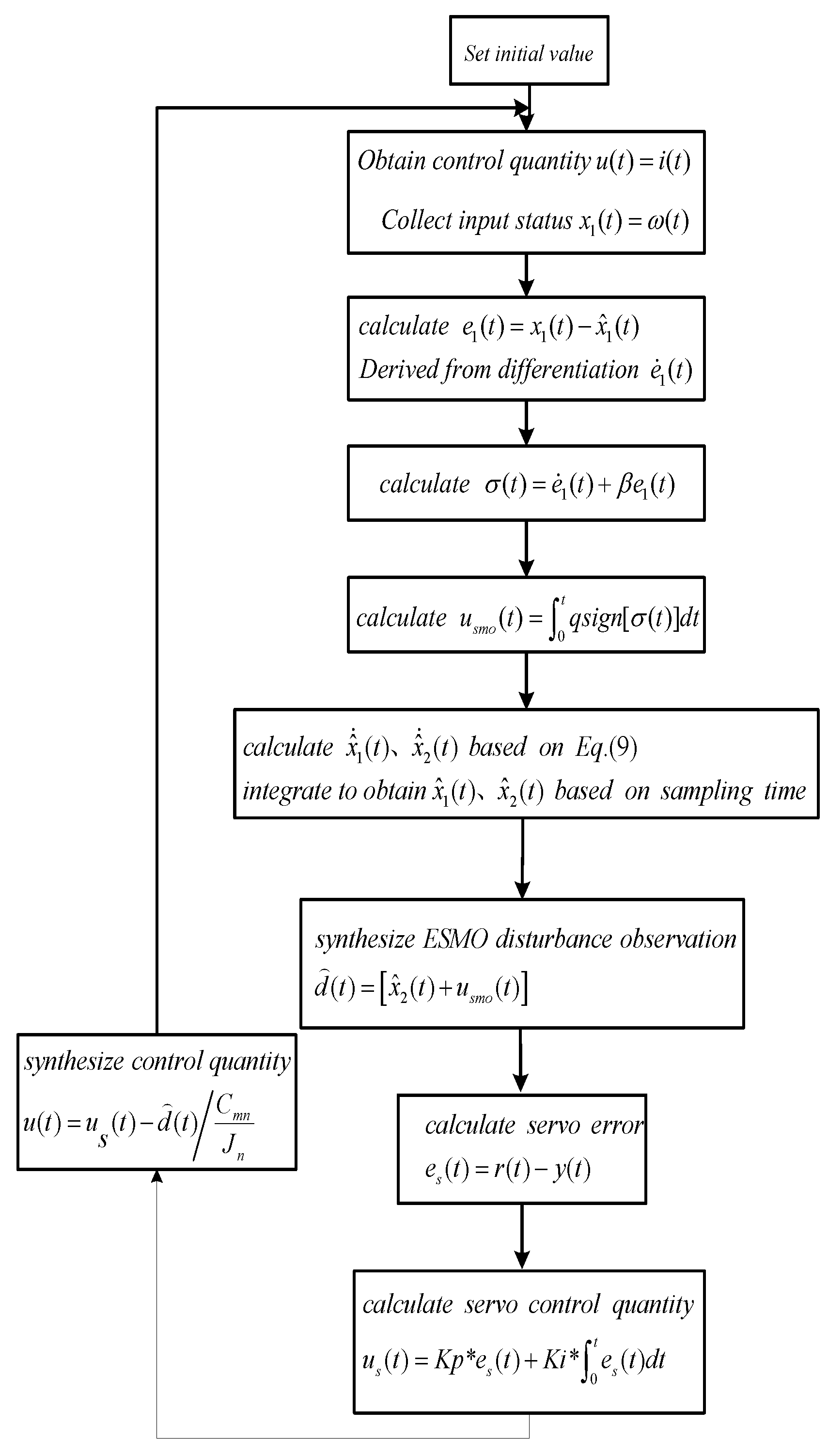
The output of the inner loop ESMO observer is compensated to the controller output, while the outer loop controller $G_c\left(s\right)$ uses a proportional integer (PI) control rate to further suppress disturbances. The system input r(t) = 0 and operates in stable mode. At the same time, in order to approach the actual system more realistically, based on the actual noise characteristics of the system, in the simulation, Band Limited White Noise is introduced at the output position of the system to simulate system noise, which follows an N(0, 0.00142) distribution. The flowchart of the control algorithm is shown in Figure 2.

(a) 

Sinusoidal Disturbance Simulation and Analysis

Most conventional disturbance estimation studies focus on disturbances in the 1–2 Hz range. To verify the estimation effect on rapidly changing disturbances, this simulation uses an 8 Hz sinusoidal disturbance as a representative to evaluate the ESMO disturbance estimation effect. The sinusoidal disturbance is $d\left(t\right)=18sin\left(16\pi t\right)$ and $\dot{d}\left(t\right)=288\pi sin\left(16\pi t\right)$. In this condition, the upper bound of $\left|\dot{d}\left(t\right)\right|$ is 288π, which is less than p = 920.

To compare the algorithm’s effectiveness, it was compared with the conventional LESO algorithm and the SMO method from [25]. The tracking differentiator is used in SMO method [25] to obtain the estimates of $\mathsf{\omega }\left(\mathrm{t}\right)$ and $\mathrm{u}\left(\mathrm{t}\right)$. The aim of Equation (44) is to map ${\widehat{\mathrm{y}}}_1\left(\mathrm{t}\right)\to \mathsf{\omega }\left(\mathrm{t}\right)$ and ${\widehat{\mathrm{y}}}_2\left(\mathrm{t}\right)\to \dot{\mathsf{\omega }}\left(\mathrm{t}\right)$, where ${\widehat{\mathrm{y}}}_1\left(\mathrm{t}\right)$ and ${\widehat{\mathrm{y}}}_2\left(\mathrm{t}\right)$ are the sate values. The aim of Equation (45) is to map ${\widehat{\mathrm{y}}}_3\left(\mathrm{t}\right)\to \mathrm{u}\left(\mathrm{t}\right)$ and ${\widehat{\mathrm{y}}}_4\left(\mathrm{t}\right)\to \dot{\mathrm{u}}\left(\mathrm{t}\right)$, where ${\widehat{\mathrm{y}}}_3\left(\mathrm{t}\right)$ and ${\widehat{\mathrm{y}}}_4\left(\mathrm{t}\right)$ are the state values and ${\mathsf{\alpha }}_1$, ${\mathsf{\alpha }}_2$, and R are the tracking differentiator weighting coefficients.

$$\left\{\begin{array}{c}{\dot{\widehat{y}}}_1\left(t\right)={\widehat{y}}_2\left(t\right)\\ {\dot{\widehat{y}}}_2\left(t\right)=-R^2{\alpha }_1\left[{\widehat{y}}_1\left(t\right)-\omega \left(t\right)\right]-R{\alpha }_2{\widehat{y}}_2\left(t\right)\end{array}\right.$$

(44)

$$\left\{\begin{array}{c}{\dot{\widehat{y}}}_3\left(t\right)={\widehat{y}}_4\left(t\right)\\ {\dot{\widehat{y}}}_4\left(t\right)=-R^2{\alpha }_1\left[{\widehat{y}}_3\left(t\right)-u\left(t\right)\right]-R{\alpha }_2{\widehat{y}}_4\left(t\right)\end{array}\right.$$

(45)

Furthermore, the disturbance estimation ${\widehat{\mathrm{d}}}_{\mathrm{n}}\left(\mathrm{t}\right)$ is obtained, as shown in Equation (46). Based on the disturbance estimation, the SMO observer ${\mathrm{u}}_{\mathrm{t}}\left(\mathrm{t}\right)$ is introduced, as shown in Equation (47). The sliding mode surface of the SMO ${\sigma }_n\left(t\right)$ is given by Equation (49) and the estimation error by Equation (48). The sliding reaching law can be expressed as Equation (50), where $\mathsf{\xi }$ is the SMO approach rate coefficient. And its switching gain is showed as Equations (51) and (52), where $\mathsf{\Gamma }$ is the sliding mode switching gain and $\mathsf{\gamma }$ is the sliding mode surface coefficient

$${\widehat{d}}_n\left(t\right)={\widehat{y}}_2\left(t\right)-{\displaystyle \frac{c_{mn}}{J_n}}{\widehat{y}}_3\left(t\right)$$

(46)

$$J_n {\dot{\omega }}_t\left(t\right)=C_{mn}u\left(t\right)+J_n{\widehat{d}}_n\left(t\right)+C_{mn}{u}_t\left(t\right)$$

(47)

$$e_n\left(t\right)=\omega \left(t\right)-{\omega }_t\left(t\right)$$

(48)

$${\sigma }_n\left(t\right)={\dot{e}}_n\left(t\right)$$

(49)

$$u_t\left(t\right)=\xi {\sigma }_n\left(t\right)+\phi \left(t\right)sign[{\sigma }_n\left(t\right)]$$

(50)

$$\phi \left(t\right)=\left\{\begin{array}{c}\Gamma ,{\sigma }_n\left(t\right)>\gamma \\ {\widehat{y}}_5\left(t\right),\left|{\sigma }_n\left(t\right)\right|\le \gamma \end{array}\right.$$

(51)

where $t_0$ is the time when $\left|{\sigma }_n\left(t\right)\right|$ changes from greater than γ to less than or equal to γ.

$$\left\{\begin{array}{c}{\dot{\widehat{y}}}_5\left(t\right)={\widehat{y}}_6\left(t\right),{\widehat{y}}_5\left(t_0\right)=\Gamma \\ {\dot{\widehat{y}}}_6\left(t\right)=-R^2{\alpha }_1{\widehat{y}}_5\left(t\right)-R{\alpha }_2{\widehat{y}}_6\left(t\right),{\widehat{y}}_6\left(t_0\right)=0\end{array}\right.$$

(52)

Simulation experiment parameters of sinusoidal disturbance are shown in

Table 1. The simulation experiment parameters of sinusoidal disturbance.

Symbol	Description	Values
$J$	inertia J	0.01 kg‧m2
$C_{mn}$	Torque coefficient	$0.2\mathrm{Nm}/\mathrm{A}$
Kp	Proportional gain in $G_c\left(s\right)$	93.6
Ki	Integral gain $G_c\left(s\right)$	150
${\omega }_o$	LESO bandwidth of the proposed method	$2\times \pi \times 29.8 \mathrm{H}\mathrm{z}$
q	Switching gain of the proposed method	920
Kp1	Controller proportional gain [25]	4.68
Ki1	Controller integral gain [25]	7.5
R	Tracking differentiator coefficient [25]	200
${\alpha }_1$	Tracking differentiator weighting coefficient [25]	1
${\alpha }_2$	Tracking differentiator weighting coefficient [25]	2
$\xi$	SMO approach rate coefficient [25]	5
$\Gamma$	Sliding mode switching gain [25]	1.25
$\gamma$	Sliding mode surface coefficient [25]	0.027

.

Figure 3 shows the sinusoidal disturbance estimation. Due to the constraints of actual system noise, the observation bandwidth ${\mathsf{\omega }}_{\mathrm{o}}$ of the LESO cannot be infinitely large. Therefore, as the disturbance bandwidth increases, the observation error, especially the phase lag of the LESO, will increase. From the disturbance simulation results in Figure 3a, it can be seen that under 8 Hz sinusoidal disturbance, overall, the LESO method exhibits a noticeable lag in estimating rapidly changing disturbances. The SMO contains a fast switching convergence feature shown as in Equations (14) and (50), and can observe wide-band and rapidly changing disturbances. After introducing the SMO, both the adaptive SMO in [25] method and the ESMO method proposed in this paper improved the estimation capability for rapidly changing disturbances, with no significant estimation lag observed for rapidly changing disturbances. However, when ${\sigma }_n\left(t\right)>\gamma$ in the adaptive SMO [25], the switching gain is a fixed large value, and the switching gain is greater than the upper bound of disturbance. When ${\sigma }_n\left(t\right)$ changes from greater than γ to less than or equal to γ, the switching gain gradually decreases from $\mathsf{\Gamma }$, and there is a dynamic process of the switching gain gradually decreasing. So, the adaptive SMO method shows noticeable chattering in the estimation results during disturbance gain switching, and the magnitude of chattering depends on the gain setting. Figure 3b shows that the maximum estimation error of the LESO is about 0.1 Nm, while the adaptive SMO method has a larger estimation error of about 0.3 Nm during switching gain adjustments, and after the gain adjustment, the estimation error is about 0.03 Nm. The method proposed in this paper observes wide-band and rapidly changing disturbances utilizing the rapidly switching characteristic of the SMO shown in Equation (14) and smooths the jitter of the SMO by cascading sliding mode estimation to the differentiation term of extended observation, achieving the integral effect of the reaching law. The method proposed in this paper shows a disturbance estimation error of less than 0.01 Nm.

Figure 3c shows that the proposed method’s σ(t) is finite and fluctuates around zero, thereby proving Theorem 1, confirming the existence of the sliding mode state in Theorem 1. Figure 3d compares the chattering effects of the control value between the adaptive SMO and ESMO methods. It shows that the adaptive SMO has significant chattering up to 1.5 A during the gain-switching process, with a control input chattering of 0.04 A after the switching process. This chattering is consistent with the noticeable chattering in the estimation results during disturbance gain switching. The ESMO method, utilizing the low-pass effect of the LESO, has better smoothing of the chattering, with a control input chattering of 0.02 A. Figure 3e compares the stability accuracy of the three methods under the sinusoidal disturbance. The stability accuracy error is 0.09 rad/s for the LESO, 0.015 rad/s for the adaptive SMO, and 0.004 rad/s for the ESMO. Simulation results are shown in

Table 2. The simulation results of sinusoidal disturbance.

Comparison Items	LESO	ASMO	ESMO
Estimation error	0.1 Nm	0.3 Nm (Switching gain adjustment process) 0.03 Nm (Switching gain adjustment ends)	0.005 Nm
Stability accuracy error	0.09 rad/s	0.015 rad/s	0.004 rad/s
Control value jitter	NA	1.5 A (Switching gain adjustment process) 0.04 A (Switching gain adjustment ends)	0.02 A

. The method proposed in this paper provides better disturbance estimation, resulting in the smallest servo error.

(b) 

Step Disturbance Simulation and Analysis

To verify the effectiveness of the ESMO in estimating rapidly changing disturbances when q is smaller than the upper bound of the disturbance or the upper bound of the disturbance is unknown, the disturbance is $d\left(t\right)=\left\{\begin{array}{c}0\\ 180(t-0.5)\end{array}\right.\begin{array}{c}t<0.5\\ t\ge 0.5\end{array}$, and in this condition, $\dot{d}\left(t\right)$ is a step disturbance, $\dot{d}(t)=\left\{\begin{array}{c}0\\ 180\end{array}\right.\begin{array}{c}t<0.5\\ t\ge 0.5\end{array}$, with the upper bound ${\left|\dot{d}\left(t\right)\right|}_{sup}=180$. The input for the speed loop is r(t) = 0, operating in stable mode.

During the simulation, the switching gain q is set to 920 and 100 respectively, to verify the suppression effect of the ESMO when switching gain is greater than and less than the disturbance upper bound. Except for the switching gain q, all other simulation parameters are the same as in Table 1. The simulation results are shown in Figure 4.

Figure 4a shows the estimation performance of the LESO and ESMO under step disturbance at t = 0.5 s. It can be seen that in Figure 4a, at t = 0.5 s, the LESO is limited by the observation bandwidth and cannot quickly estimate step disturbances. The ESMO works quickly as in Equation (14), outputting $u_{smo}\left(t\right)$ to achieve rapid observation of step disturbances when a step disturbance is imposed. So, the ESMO method estimates a faster response than the LESO method, and when the switching gain q of the ESMO is larger, the observer’s estimation response is faster and the error is smaller; from Figure 4b, when the switching gain q = 920 is greater than the upper bound of the disturbance, the estimation error approaches zero. When the switching gain q = 100 is less than the upper bound of the disturbance, the estimation error is 0.01 Nm, but it is still smaller than the LESO estimation error of 0.02 Nm, thus verifying Theorem 2.

From Figure 4c, it can be seen that the proposed method’s σ(t) is finite. When the switching gain q = 920 in Equation (14) is greater than the upper bound of the disturbance, σ(t) fluctuates around zero. When the switching gain q = 100 in Equation (14) is less than the upper bound of the disturbance, since the switching gain is less than the upper bound, it does not enter the sliding mode state. But the ESMO still works quickly as in Equation (14), outputting $u_{smo}\left(t\right)$. At this time, due to the reasons of $\dot{d}\left(t\right)>0$, $\sigma \left(t\right)>0$, the sliding mode observer outputs the sliding mode estimate with the maximum gain, further compensating for the LESO estimation error, which is consistent with the proof of Theorem 2 in the simulation results.

In Figure 4d, it can be seen that the control value chattering is relatively small, about 0.02 A. Figure 4e compares the stability accuracy errors of the ESMO and LESO methods under the step disturbance, showing that ESMO has smaller servo errors. As the switching gain q in the ESMO increases, the error decreases. When q = 920, which is greater than the upper bound of the disturbance, the disturbance is quickly estimated and compensated, and the system servo error remains around zero. When q = 100, the ESMO cannot fully compensate for the disturbance, and the remaining part is compensated by the outer controller $G_c\left(s\right)$. The stability accuracy error of the ESMO gradually decreases from 0.01 rad/s. The LESO disturbance estimation error is larger than that of the ESMO, with most disturbances needing compensation by the outer controller $G_c\left(s\right)$, and the stability accuracy error of the LESO gradually decreases from 0.02 rad/s. Simulation results are shown in

Table 3. The simulation results of step disturbance.

Comparison Items	LESO	ESMO q = 100	ESMO q = 920
Estimation error	0.02 Nm	0.01 Nm	<0.001 Nm
Stability accuracy error	0.02 rad/s gradually decreases	0.01 rad/s gradually decreases	<0.001 rad/
Controlled variable jitter	NA	NA	0.02 A

.

6. Conclusions

This paper investigates the problem of estimating and accurately compensating for wide-band, rapidly changing disturbances, and proposes an ESMO method. An SMO is introduced into the disturbance term estimated by the LESO, utilizing the switching characteristic of sliding mode to compensate for the inadequacies of the LESO in observing rapidly changing disturbances. The proposed method smooths the jitter of the SMO by cascading sliding mode estimation to the differentiation term of extended observation, achieving the integral effect of the reaching law. At the same time, the influence of chattering is considered as part of the ‘total disturbance’, and observed by the ESO to achieve fast and accurate estimation of the ‘total disturbance’. The stability and convergence characteristics of the proposed method are mathematically proved, revealing that it operates stably without knowing the disturbance’s upper bound and offers faster dynamics and higher accuracy than the LESO. Its effectiveness is verified through the simulation experiments. The results show that the proposed method improves the observation ability for wide-band and rapidly changing disturbances, improving the observation accuracy of disturbances and enhancing the disturbance suppression ability of the system. In addition to the ${\mathsf{\omega }}_o$ of the LESO, this method only requires to tune one switching gain parameter q, making it simple and convenient to debug and easy for engineering applications. The method can be used for disturbance estimation and compensation in optical inertial stabilized platform control systems to observe disturbances, improving stability accuracy.

This method is a general observer scheme. Future research can explore its application to other high-order systems, and the extended observer can be combined with other forms of SMO to form various types of ESMO.