Fault-Tolerant Closed-Loop Controller Using Online Fault Detection by Neural Networks

Abstract

This paper presents an online model-free sensor fault-tolerant control scheme capable of tolerating the most common faults affecting an induction motor. This approach involves using neural networks for fault detection to provide the controller with sufficient information to counteract adverse consequences due to sensor faults, such as degradation in performance, reliability, and even failures in the control system. The proposed approach does not consider the knowledge of the nominal model of the system or when the fault may occur. Therefore, a high-order recurrent neural network trained online by the Extended Kalman Filter is used to obtain a mathematical model of the system. The obtained model is used to synthesize a discrete-time sliding mode control. Then, the fault-detection and -isolation stage is performed by independent neural networks, which have as input the signal from the current sensor and the position sensor, respectively. In this way, the neural classifiers continuously monitor the sensors, showing the ability to know the sensor status. The combination of controller and fault detection maintains the operation of the motor during the time of the fault occurrence, whether due to sensor disconnection, degradation, or connection failure. In fact, the MLP neural network achieves an accuracy between 95% and 99% and shows an AUC of 97% to 99%, and this neural network correctly classifies true positives with acceptable performance. The Recall value is high, between 97% and 99%, and the F1 score confirms a good performance. In contrast, the CNN shows a higher accuracy, between 96% and 99% in accuracy and 98% to 99% in AUC. In addition, its Recall and F1 reflect a better balance and capacity to handle complex data, demonstrating its superiority to MLP in fault classification. Therefore, neural networks are a promising approach in areas such as fault-tolerant control.

1. Introduction

In recent years, there has been increasing interest in fault-tolerant control systems, motivated by the complexity of the systems to be managed and by the fact that the various components of the system can generate uncertainties, disturbances, or risks [1,2]. In general, a failure in a system can be defined as a deviation of a parameter from its acceptable value that can cause a reduction in, or loss of, the capability of a functional unit to perform a required function. In this way, fault tolerance is interpreted as the ability of a system to continue functioning despite the presence of faults. The presence of faults is inevitable in any real system, and this can cause impairments in the stability and performance of the system.

The operation of faulty systems mitigates system performance, but the degradation may be acceptable up to a certain level of confidence. Such approaches that are capable of providing system safety and reliability by mitigating the effects of system failures or breakdowns are called fault-tolerant control (FTC) systems [3,4]. Fault-tolerant control schemes are an integral part of all safety-critical systems for many of the systems with real-world applications such as engines. FTC consists of the following phases.

The primary stage is fault detection and isolation (FDI), which is to process the system’s input–output data to find faults. In addition to detecting the fault, FDI is responsible for isolating it from other possible faults present to facilitate precise and efficient intervention [5]. Then, an adjustment is made to the fault-tolerant control algorithm to compensate for the effects caused by the detected fault, using the information obtained during the detection and isolation phase. In this way, it is guaranteed that the system can continue to operate safely and efficiently, despite the presence of faults, maintaining its performance within acceptable margins [3].

FDI is indispensable for fault-tolerant control systems because it provides information about faults, which enables control capable of reducing or eliminating negative impacts on system performance. Therefore, FDI is an important field of research in all types of systems. Numerous studies have been dedicated to fault detection and isolation. However, most FDI schemes are model-based, using nominal, fault-free mathematical representations of the system.

Model-based schemes use the residual generated by the difference between plant sensor measurements and signals generated by a mathematical model. Therefore, if this residual is too large and exceeds a predefined threshold, then an alarm is triggered. In order to prevent false alarms brought on by signal noise or disruptions, this threshold was carefully chosen. An example of a model-based technique in the paper [6] addresses the problem of isolation, diagnosis, and fault-tolerant control in quadrotor UAV systems with uncertainties. A general dynamic model is proposed that considers uncertainties in the system state and input. The work uses an observer method to identify faults, followed by an adaptive observer that accurately estimates the magnitude of the faults. The estimate is then used by a fault-tolerant controller based on sliding modes to compensate for the faults and ensure that the system output follows the desired reference signals, even in the face of external disturbances and actuator failures. The effectiveness of the methodology is validated through simulations. Also, in the article [7], model-based fault detection and isolation are addressed. It focuses on distributed parameter systems (DPSs) modeled by parabolic partial differential equations (PDEs). For fault detection, a filter-based scheme is proposed that allows the detection of faults in actuators, sensors, and states in linear and non-linear systems based on Luenberger-type observers with filters to generate residuals to detect the fault. The paper [8] addresses the problem of fault detection and isolation (FDI) of sensors in networks of linear process systems with a loop structure. A dynamic model based on a two-input, single-output LTI state-space model is proposed that incorporates faults as additive linear terms. The fault isolation algorithm is able to detect faulty measurements in the network. Furthermore, a proportional-integral (PI)-based observer is developed to estimate the magnitude of the faults. The proposed method is validated in MATLAB/Simulink.

In model-free schemes, the system’s state variables are monitored by employing measured data without establishing explicit dependency laws. From these principles, an accurate model is obtained. The development of this type of approach is based on measurements of the input and output variables of the process. Data are collected from the plant, both under normal conditions and in the presence of faults [9].

In this work, a real-time fault diagnosis and isolation scheme is proposed using neural networks to provide information to control systems about the presence of faults. There are various classification techniques to solve fault-detection and -isolation problems in control systems, such as probabilistic methods and “black box” approaches [10,11], as well as artificial neural networks (ANNs), support vector machines (SVMs), and fuzzy inference [12]. A promising approach is using deep neural networks (DNNs) for fault classification and isolation. By employing currents, vibrations, or voltages as input to the model, DNNs have been used to detect faults in circuits or motors, improve maintenance and detect early faults in machinery gears [13,14,15].

In model-free adaptive control approaches, the controller is designed using observed input and output data of a plant. Assumptions like unmodeled dynamics or theoretical preconceptions regarding plant dynamics are eliminated because nominal plant models are not necessary [16]. Under this circumstance, controller design is considered a controller-parameter-identification problem.

For this purpose, artificial neural networks (ANNs) have gained relevance in identifying mathematical models accurately, allowing them to predict, simulate, emulate, and even design [17] control systems. These models identified by neural networks approximate nonlinear dynamics, along with perturbations, which are then used to synthesize conventional [18] controllers.

This work presents a fault-tolerant control scheme that fully utilizes neural networks for its implementation, from system identification to fault detection and isolation, using sliding mode control for discrete-time nonlinear systems. In general, works related to fault-tolerant control (FTC) are model-based. However, in this work, both the controller and the fault classifier are considered model-free, making it an attractive approach within artificial intelligence.

The proposed methodology for neural classification on faulty sensor data streams and fault-tolerant control is applied to an induction motor. The fault-tolerant control and fault detection and isolation schemes are implemented in a closed loop using deep neural network architectures without knowledge of a nominal motor model. The contributions of the work are highlighted below.

• Sensor fault classification is performed in real time using two deep neural networks.
• The classification is performed using neural classifiers without pre-processing the data.
• The neural classifiers and the controller are tested in a closed loop in MATLAB/Simulink Version: 24.2.0.2790852 (R2024b) Update 2.
• A real-world application is included in the fault-tolerant control (FTC) scheme.
• The fault classification results between a multilayer perceptron (MLP) neural network and a convolutional neural network (CNN) are compared.
• A high-order recurrent neural network (RHONN) was used to identify the model of an induction motor, and the Extended Kalman Filter (EKF) was used as a training algorithm to obtain an adequate model despite unexpected conditions such as disturbances or sensor failures.
• A sliding mode control for discrete-time nonlinear systems was used to control the motor in the presence of faults.

The paper is organized as follows: first, a review of the analyzed system is included. Next, the proposed neural networks that will be used as fault classifiers are described. Then, the proposed scheme for fault detection and isolation is presented. Then, the RHONN for system identification is described, together with the sliding mode controller. Next, the results obtained are presented and discussed, and finally, conclusions and future work are presented.

2. Review of the Analyzed System

Induction motors (IMs) have diverse applications in industry and in real-world applications because they are reliable, low-cost, and efficient tools [4,19,20]. Electric motor applications subject them to long periods of work under electrical and mechanical stress conditions, which can cause failures or malfunctions, negatively affecting their stability and efficiency. For this reason, it is crucial to detect failures quickly and accurately to take corrective measures that preserve safety and performance and then prevent major failures [21,22]. There are three types of failures in induction motors: converter, machine, and sensor. Among them, the sensor has the greatest potential for failure, and since its function is to monitor the system’s state variables, it is crucial for control applications.

Control of induction motors (IMs) often relies on feedback signals such as rotor position and currents in stator coordinates $\alpha$-$\beta$. The transformed voltage vector rotates with the power supply frequency, and its components are projected onto the $\alpha$-$\beta$ axes. However, faults caused in these sensors negatively affect system performance, which could lead to total system failure. Current sensors are usually the most prone to failure, but malfunctions can also occur in other speed or position sensors.

The state variables considered measurable are $\theta$ for the rotor position, $\omega$ for its speed, $i_{\alpha }$ and $i_{\beta }$ for the alpha and beta currents, respectively, and ${\varphi }_{\alpha }$ and ${\varphi }_{\beta }$, representing the alpha and beta fluxes, respectively [23].

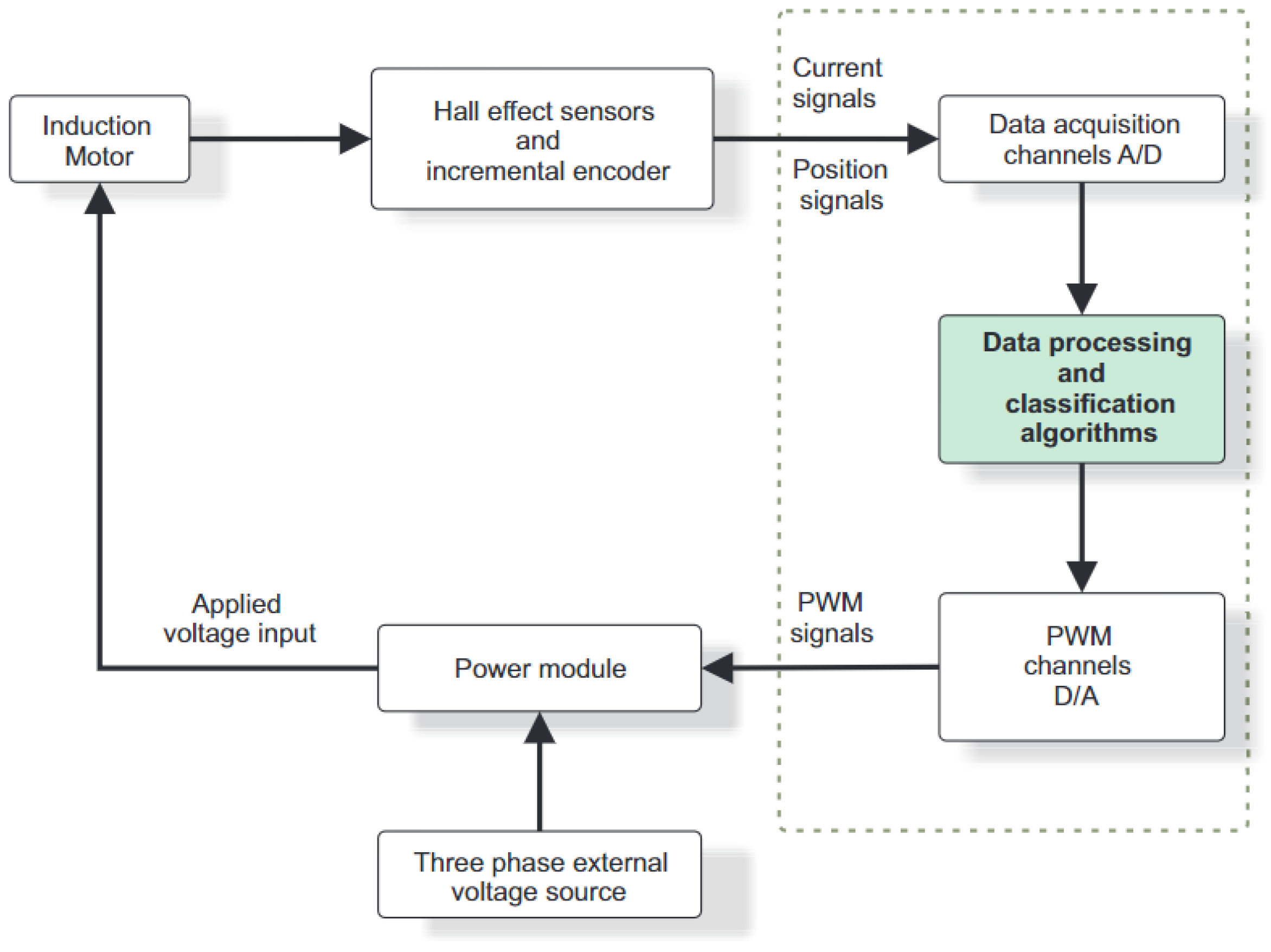
For this work, faults in current and position sensors are considered, and multilayer perceptron neural networks and convolutional neural networks perform fault detection. Then, system identification is carried out by a high-order recurrent neural network (RHONN), which is trained online; the obtained model synthesizes a discrete-time sliding-mode controller. The configuration used is shown in Figure 1. The proposed scheme is simulated and tested in MATLAB/Simulink Version: 24.2.0.2790852 (R2024b) Update 2, under various operating conditions.

3. Deep Neural Networks

Online sensor fault detection requires methods capable of analyzing large volumes of data in real time to achieve rapid and accurate detection. Common methods for sensor fault detection rely on observers, who rely on accurate mathematical models of the system being observed. However, in real-world applications, system parameters tend to vary over time. In addition, unknown perturbations can cause false alarms, making this approach ineffective [24].

There are FDI methods that have used neural networks, but they have shallow architectures, which limits their ability to learn complex non-linear relationships [11].

In contrast, deep neural networks (DNNs) have more complex architectures due to multiple layers of nonlinear operations, enabling them to capture complex functions through the training of those layers. [25]. In fault detection and isolation problems, DNNs can learn the characteristics of healthy or defective sensors, employing only the observed data from the sensors.

For FDI problems, deep neural networks have the ability to learn the characteristics of a healthy state or a fault state using only data observed over time by sensors. These characteristics allow the development of more reliable and effective fault diagnosis systems, overcoming the shortcomings of current methods for FDI.

Therefore, in this work, two neural networks are proposed to carry out online fault classification and isolation using the observed data from current sensors ($\alpha$ and $\beta$) and the position sensor in a fast and accurate manner. The proposed neural networks are the MLP neural network and the convolutional neural network, which are described below.

3.1. Multilayer Perceptron Networks

One of the widely recognized and used neural networks in various research fields is the MLP. It has applications such as in the problems published in [26,27], and it especially stands out for its efficiency and flexibility in classification tasks [27]. Its basic architecture generally consists of an input layer, one or more hidden layers, and an output layer in feed-forward mode. Dense layers comprise two or more hidden layers, each composed of several nodes, which are connected to the nodes of the adjacent layers through their corresponding weights.

The output of the network $y_p$ is obtained by adding the m neurons of the hidden layer, each multiplied by the inputs $u_n$ and the weights W, as shown in the following equation:

$$y_p=\sigma (\sum W_{nm}\sigma (\sum W_{nn}{u}_n+b_1)+b_2)$$

(1)

where m is the number of neurons, $u_n$ represents the input vector, $\sigma$ is the activation function, $W_{nn}$ corresponds to the weight matrix of the hidden layer, $W_{nm}$ is the weight matrix of the second layer, and $b_1$ and $b_2$ are the bias values.

3.2. Convolutional Neural Network

Convolutional neural networks (CNNs) have proven to be effective and widely used tools in various applications such as object recognition and image classification due to their ability to extract complex features from visual data. In recent years, their use has also been extended to the field of fault detection and classification, where CNNs help to identify anomalous patterns and improve the accuracy of problem diagnosis [28,29,30,31,32].

Although CNN applications are focused on 2D images or where information can be represented in two-dimensional matrices, 1D convolution architectures have also been used. These architectures use one-dimensional kernels and filters on the input signal. However, there are not many works that use this architecture with online applications in classification tasks.

A CNN is built from three main layers: a filter bank layer, a nonlinearity layer, and a feature pooling layer [33].

The filter bank layer is responsible for applying various filters to the input data. The output of the layer is generated by convolving the weights of the neurons (also known as filters or kernels) with the input data, resulting in an activation map. The resulting activation maps are stacked to form an output volume [34].

The nonlinearity layer uses the Rectified Linear Unit (ReLU) nonlinear function to adjust the generated output. The ReLU function is expressed by the following equation:

$$ReLU=\left\{\begin{array}{cc}0,& ifv<0,\\ \\ v,& ifv\ge 0.\end{array}\right.$$

(2)

In the pooling layer, the dimension of the input data is reduced. The most frequently applied methods are max pooling and mean pooling. Finally, in the output layer, the softmax function is used to maximize the probability of the output classes [34]. The equation of the Softmax function is expressed as follows:

$$o_j={\displaystyle \frac{e^{v_j}}{{\sum }_{j=1}^M{e}^{v_j}}},$$

(3)

where M represents the total number of output nodes, v is the output of the network before applying the softmax function, and o is the output of the network after applying the softmax function.

4. Neural Identifier

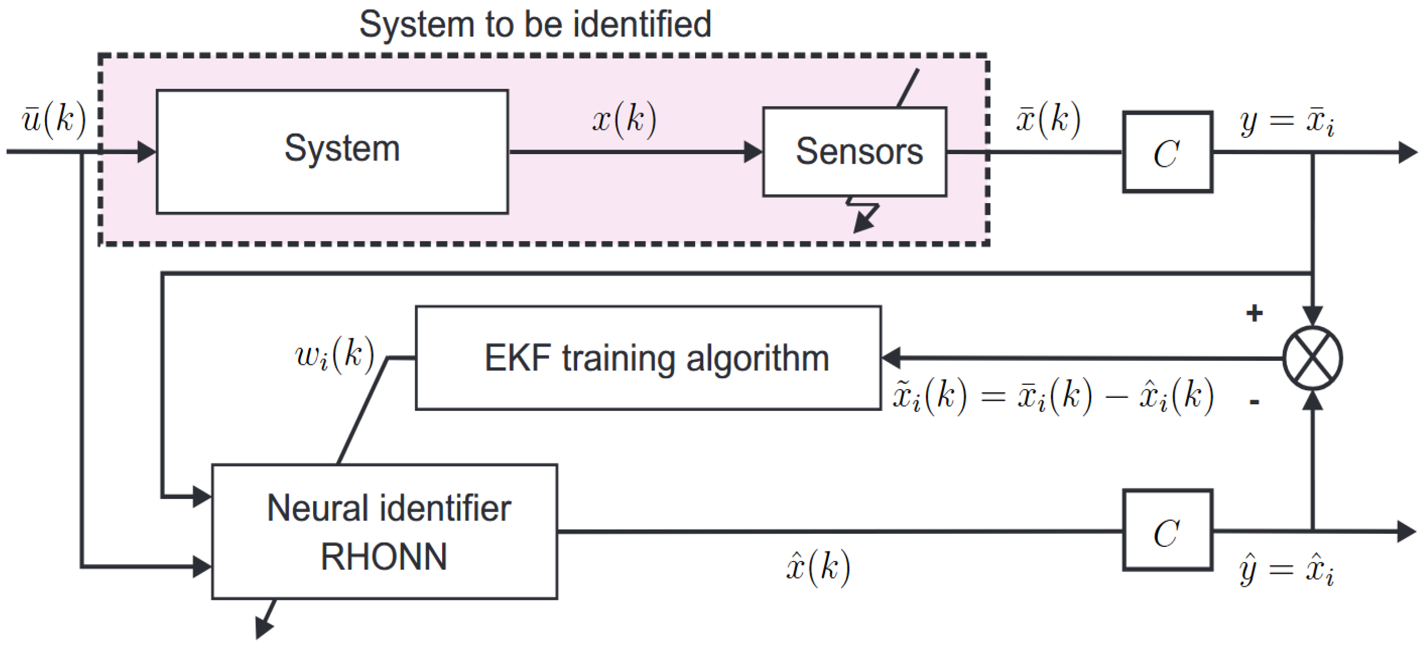
Figure 2 shows the methodology implemented in the identification of the nonlinear model with uncertainties, external disturbances, and sensor failures. In addition, the neural controller used to control the system in the presence of sensor failures is shown. The structure of a model identification system that integrates a Recurrent High-Order Neural Network (RHONN) and an Extended Kalman Filter (EKF). This scheme is used to estimate the state of a nonlinear dynamical system.

Let us consider an unknown nonlinear system that is subject to sensor failures. The complete system can be described as follows:

$$\overline{x}(k+1)=G(\overline{x}\left(k\right),\overline{u}\left(k\right))+\Delta \left(k\right)$$

(4)

$$y\left(k\right)=C\overline{x}\left(k\right)$$

(5)

where $\overline{x}\in {\mathbb{R}}^n$ represents the state vector of the system, $\overline{u}\in {\mathbb{R}}^m$ is the control signal applied, $y\in {\mathbb{R}}^p$ is the output vector, $C\in {\mathbb{R}}^{p\times m}$ is a known output matrix, $G\in {\mathbb{R}}^n\times {\mathbb{R}}^m\to {\mathbb{R}}^n$ is a nonlinear function, and $\Delta \in {\mathbb{R}}^n$ is the disturbance vector. Equation (4) can be rewritten in component-wise form:

$${\overline{x}}_i(k+1)=G_i(\overline{x}\left(k\right),\overline{u}\left(k\right))+{\Delta }_i\left(k\right)i=1,2,\dots ,n$$

(6)

Sensor faults can be defined as

$$\overline{x}\left(k\right)={\psi }_i(x_i\left(k\right),{\gamma }_i\left(k\right))$$

(7)

where ${\psi }_i$ is an unknown nonlinear function that depends on the sensor signal and is considered unknown but bounded. This function reflects the loss of sensor efficiency due to external inputs not measurable by the system, such as biases, drifts, or loss of accuracy over time $k_i^{*}$. $x_i\left(k\right)$ is assumed to be a measurable variable, and its measurement is denoted as ${\overline{x}}_i\left(k\right)$. The identification of the system is given in Equation (7) using a high-order recurrent neural network (RHONN).

In the context of sensor fault detection, the characteristics of the vectors $\overline{x}$ representing the internal dynamics of the system (4) can result in two distinct outcomes: either “failed” or “healthy”. Consequently, this scenario can be viewed as a classification problem, characterized by

$${\psi }_i(x_i\left(k\right),{\gamma }_i\left(k\right))=\left\{\begin{array}{c}failure,{\psi }_i\left(*\right)\in \Gamma \\ non-failure,{\psi }_i\left(*\right)\notin \Gamma \end{array}\right.$$

(8)

where $\Gamma$ represents the set of all possible failure modes. This set $\Gamma$ is then considered partially known due to the difficulty of completely defining the nonlinear system.

If the complete state $x\left(k\right)$ of the system is available and there is a data structure in the dynamics of (8), they can be recognized as features in a time series.

So, we can say that it is feasible to identify a “failure scenario” in the system by combining all input signals into a univariate time series.

4.1. Recurrent High-Order Neural Networks

The RHONN is useful for control tasks [35]. The ideal RHONN is

$${\overline{x}}_i(k+1)=w_i^{*T}{z}_i(\overline{x}\left(k\right),\overline{u}\left(k\right))+{ϵ}_{zi}i=1,2,\dots ,n$$

(9)

where $w^{*}i$ is the vector of ideal weights and $z_i(\overline{x}\left(k\right),\overline{u}\left(k\right))$ is a vector containing $L_i$ high-order terms, as described by [36]. Also, ${ϵ}_{zi}$ is the bounded approximation error that depends on the number of adjustable weights [36].

$$z_i(\overline{x}\left(k\right),\overline{u}\left(k\right))=\left[\begin{array}{c}{z}_{i_1}\\ z_{i_2}\\ ⋮\\ z_{i_{L_i}}\end{array}\right]=\left[\begin{array}{c}{\displaystyle \prod _{j\in I_1}{\xi }_{ij}^{r_{ij}^{\left(1\right)}}}\\ {\displaystyle \prod _{j\in I_2}{\xi }_{ij}^{r_{ij}^{\left(2\right)}}}\\ ⋮\\ {\displaystyle \prod _{j\in I_{L_i}}{\xi }_{ij}^{r_{ij}^{\left(L_i\right)}}}\end{array}\right]$$

(10)

with $r_{ij}\left(k\right)$ being non-negative integers and ${\xi }_i$ is defined as follows:

$${\xi }_i=\left[\begin{array}{c}{\xi }_{i_1}\\ ⋮\\ {\xi }_{i_n}\\ {\xi }_{i_{n+1}}\\ ⋮\\ z_{i_{n+m}}\end{array}\right]=\left[\begin{array}{c}S\left(x_1\right)\\ ⋮\\ S\left(x_n\right)\\ {\overline{u}}_1\\ ⋮\\ {\overline{u}}_m\end{array}\right]$$

(11)

in Equation (11), $\overline{u}=[{\overline{u}}_1,{\overline{u}}_2,\dots ,{\overline{u}}_m]$ is the input vector to the neural network, and $S(·)$ is:

$$S\left(\varsigma \right)={\mu }_{i}tanh\left({\beta }_i\varsigma \right)$$

(12)

where $\varsigma$ is a real value variable and $\mu$, $\beta$ are positive constants.

The ideal weight vector $w^{*}$ is assumed to be minimized together with $|{ϵ}_{zi}|$ on a compact set ${\Omega }_{zi}\supset {\mathbb{R}}^{L_i}$. For the purposes of analysis, the vector $w_i^T$ is assumed to exist and is constant and unknown. Therefore, by defining $w_i$ as an estimate of $w_i^{*}$, one can approximate the ideal RHONN as follows:

$${\widehat{x}}_i(k+1)=w_i^T{z}_i(\overline{x}\left(k\right),\overline{u}\left(k\right))+{ϵ}_{zi}i=1,2,\dots ,n$$

(13)

Then, the estimation error of the weights is defined as

$$\begin{array}{c}\hfill {\tilde{w}}_i\left(k\right)=[w_i^{*}\left(k\right)-w_i\left(k\right)]\end{array}$$

(14)

Then, from (9) and (13), the identification error is defined as

$$\begin{array}{c}\hfill {\tilde{x}}_i\left(k\right)=[{\overline{x}}_i\left(k\right)-{\widehat{x}}_i\left(k\right)]\end{array}$$

(15)

where $\widehat{x}$ corresponds to the output generated by the neural network and n represents the number of state variables.

4.2. RHONN Training Algorithm

The Extended Kalman Filter (EKF) algorithm is a widely used algorithm for RHONN weight optimization due to its fast convergence. The fundamental objective is to minimize the difference between the state variables of the system and those produced by the neural network. The EKF-based algorithm is described below:

$$\begin{array}{c}{w}_i(k+1)=w_i\left(k\right)+{\eta }_i{K}_i\left(k\right){\tilde{x}}_i\hfill \\ K_i\left(k\right)=P_i\left(k\right)+H_i\left(k\right){[R_i\left(k\right)+H_i^T\left(k\right)P_i\left(k\right)H_i]}^{-1}\hfill \\ P_i(k+1)=P_i\left(k\right)-K_i\left(k\right)H_i^T{P}_i\left(k\right)+Q_i\left(k\right)\hfill \end{array}$$

(16)

where $L_i$ denotes the total number of weights in the neural network, $w_i\in {\mathbb{R}}^{L_i}$ is the vector containing these weights, and $P_i\in {\mathbb{R}}^{L_i\times L_i}$ is the covariance matrix associated with the estimation error of these weights. The learning rate is represented by ${\eta }_i$, while $K_i\in {\mathbb{R}}^{L_i\times m}$ is the Kalman gain matrix. $Q_i\in {\mathbb{R}}^{L_i\times L_i}$ is the noise covariance matrix related to the estimation of the weights, and $R_i\in {\mathbb{R}}^{m\times m}$ corresponds to the measurement noise covariance matrix. Finally, $H_i\in {\mathbb{R}}^{L_i\times m}$ is defined as follows:

$$H_i\left(k\right)={\left[\begin{array}{c}{\displaystyle \frac{\partial {\overline{x}}_i\left(k\right)}{\partial w_i\left(k\right)}}\end{array}\right]}^T$$

(17)

5. Fault-Tolerant Sliding Mode Neural Controller

This study employs the RHONN neural model to develop an adaptive control law, based on the discrete-time sliding mode technique, applied to unknown nonlinear systems affected by sensor failures. According to [37], a discrete-time nonlinear system is described as follows:

$$\overline{x}(k+1)=f\left(x\left(k\right)\right)+B\left(k\right)\overline{u}\left(k\right)$$

(18)

where $\overline{x}\in {\mathbb{R}}^n$, f is a nonlinear function, $B\in {\mathbb{R}}^{nxm}$ is the input matrix, and $\overline{u}$ is the applied control law defined in Equation (23). Then, $u\in {\mathbb{R}}^m$ is the computed control law, defined as follows:

$$u\left(k\right)=\left\{\begin{array}{ccc}{u}_t\left(k\right)& for& \parallel u_t\left(k\right)\parallel \le u_{max}\\ u_{max}{\displaystyle \frac{u_t\left(k\right)}{\parallel u_t\left(k\right)\parallel }}& for& \parallel u_t\left(k\right)\parallel >u_{max}\end{array}\right.$$

(19)

with

$$u_t\left(k\right)=u_s^{eq}\left(k\right)+u_{sn}\left(k\right)$$

(20)

where $u_{max}$ is the control bound. Then, the equivalent control $u_s^{eq}$ and the stabilizing term to asymptotically reach the sliding surface $u_{sn}$ are defined as

$$\begin{array}{c}{u}_s^{eq}\left(k\right)=-B^{-1}\left(k\right)(f\left(k\right)-x^{des}(k+1))\hfill \\ u_{sn}\left(k\right)=-B^{-1}\left(k\right)K_s{S}_{mod}\left(k\right)\hfill \end{array}$$

(21)

where $K_s$ is a Schur matrix, $x^{des}$ is the desired time-varying trajectory for the state x, $B^{-1}$ is the generalized inverse of B, and the sliding surface $S_{mod}$ defined as the neural trajectory tracking error is described by:

$$S_{mod}\left(k\right)=\widehat{x}\left(k\right)-x^{des}\left(k\right)$$

(22)

It is important to note that the controller described in (23) has the ability to handle noise, uncertainties, unmodeled dynamics, and even measurement errors. For this reason, certain aspects of the control proposed in [37] have been considered to implement a fault-tolerant control scheme. First, it is assumed that faults occur in the sensors, which affect the state variables. As a result, faulty state variables replace the original measured variables. In the neural model, each $x_i$$(i=1,2,\cdots ,n)$ is replaced by ${\overline{x}}_i$$(i=1,2,\cdots ,n)$, where ${\overline{x}}_i$ corresponds to the sensor output, under computed normal or faulty conditions. With this fine-tuned neural model, the control law is synthesized as

$$\overline{u}\left(k\right)=\left\{\begin{array}{c}u\left(\overline{x}\left(k\right)\right)\mathrm{for}\overline{x}\left(k\right)\mathrm{healthy}\\ u\left(\overline{x}\left(\tau \right)\right)\mathrm{for}\overline{x}\left(k\right)\mathrm{faulty}\end{array}\right.$$

(23)

where fault occurrence is on $t=\tau$. This implies that the last value of the state variable is on hold when a fault that starts at instant $\tau$ is presented.

6. Neural-Network-Based Fault-Detection Strategy

The purpose of the FTC is to identify, correct, or reduce the impact of a fault. To this end, a controller capable of responding appropriately has been designed. In addition, an FDI scheme that works in real time and provides sufficient information to the controller is proposed. Figure 3 presents the proposed FTC scheme, which includes the induction motor, the current and position sensors, the controller, and the diagnostic process. With this configuration, the controller operates following a specific decision logic, oriented according to the fault detection and classification scheme, which allows for generating an FTC action when a fault is detected.

In industrial applications, sensors are the most susceptible to failure. However, traditional methods are affected in their efficiency by real-time processing requirements and the variable nature of the measured data. Therefore, new fault classification methods are needed that can extract valuable information from sensors, even in the presence of uncertainties, non-linear behaviors, and variability in the signals. In addition, these methods must be computationally efficient and achieve high accuracy in fault classification.

In this work, the problem of fault detection and diagnosis is addressed in two phases: a signal isolation phase and a fault classification phase. The methodology is detailed below.

For control tasks for induction motors, three sensors are usually used, two for current and one for position. In this way, fault detection and diagnosis can be approached as a multivariate time series classification problem.

In the literature, there are several methods for classifying multivariate time series, such as Dynamic Time Warping [38], whose purpose is to extract features from time series. The only drawback is that this approach presents a high computational cost when working with large data sets, which makes it unviable for real-time implementations.

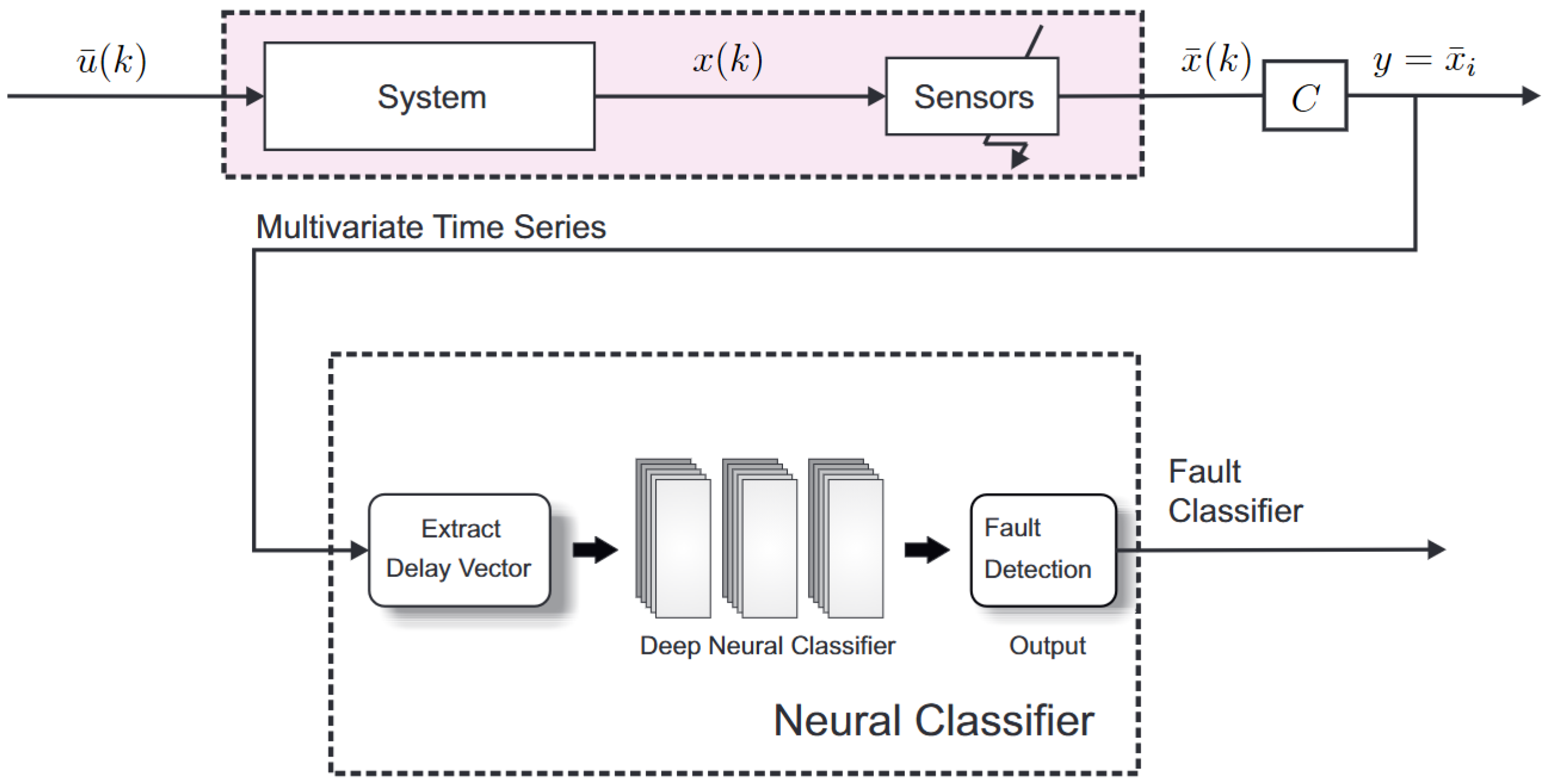
For fault detection, each sensor is monitored individually by a neural fault classifier, as shown in Figure 4. The classification results are achieved by separating the multivariate time series into univariate series, and then the univariate series are supervised by a neural classifier. The main advantage of this approach is that the neural classifier can simultaneously differentiate between failures that occur in one or more sensors without much context.

Sliding window-based strategies have been used to solve the data stream mining problem, where more relevance is given to recent information compared to historical data. In this technique, old samples are iteratively replaced with newly observed samples. This strategy is effective for fault detection, as it allows identifying faults that can occur at any time with the least number of data possible.

In this work, we propose the use of this approach since the continuous update of the current time window facilitates online fault detection to adapt to changes in system behavior over time. Data collected in overlapping time windows are used to provide additional context to [39] neural networks.

The sliding window technique divides the data into segments of length d, establishing a relationship between past and future information [40], as detailed below.

Here, we consider a univariate time series $X=[\overline{x}\left(0\right),\overline{x}\left(1\right),\overline{x}\left(2\right),\dots ,\overline{x}\left(k\right)]$ of finite length, where k is the number of samples observed so far. We obtain a sliding window $X\left(k\right)$ with length d, which captures the local information of the time series X. This window is updated iteratively as the sensor acquires new samples in real-time, i.e.,

$$X_k=[\overline{x}(k-d-1),\dots ,\overline{x}(k-1),\overline{x}\left(k\right)]$$

(24)

where $\{1,2,\dots ,d-1\}$ are lags. A graphic representation is shown in Figure 5.

The dataset D then consists of the time series $X_m$ and its corresponding class label vector $Y_m$.

$$D=(X_0,Y_0),(X_1,Y_1),\dots ,(X_k,Y_k)$$

(25)

where q represents the number of classes of $Y_m$, such that each element $j\in [1,q]$ is 1 if it corresponds to a class of $X_m$ and 0 otherwise.

7. Results

In this section, we present the results obtained with two neural classifiers, applying the previously described sensor-fault-tolerant controller scheme in neural sliding mode. The complete induction motor model, together with the controller and the neural classifier, is implemented in Matlab/SIMULINK to carry out the closed-loop system tests.

7.1. Neural Identifier

The proposed neural model for a three-phase induction motor is designed as in (13). In order to define the neural model, only the previously determined state variables are considered. The proposed RHONN model is defined to obtain a block control form [23,41] as follows:

$$\begin{array}{ccc}\hfill {\widehat{x}}_1\left(k+1\right)& =& w_{11}\left(k\right)S\left(\theta \left(k\right)\right)+w_{12}\left(k\right)S\left(\omega \left(k\right)\right)\hfill \\ \hfill {\widehat{x}}_2\left(k+1\right)& =& w_{21}S\left(\omega \left(k\right)\right)-w_{21}^{\prime }S\left({\varphi }_{\beta }\left(k\right)\right)i_{\alpha }\left(k\right)\hfill \\ & +& w_{22}^{\prime }S\left({\varphi }_{\alpha }\left(k\right)\right)i_{\beta }\left(k\right)\hfill \\ \hfill {\widehat{x}}_3\left(k+1\right)& =& w_{31}\left(k\right)S\left({\Phi }_m\left(k\right)\right)\omega \left(k\right)\hfill \\ & +& w_{32}\left(k\right)S\left({\varphi }_{\beta }\left(k\right)\right)i_{\alpha }\left(k\right)\hfill \\ & +& w_{33}\left(k\right)S\left({\varphi }_{\alpha }\left(k\right)\right)i_{\beta }\left(k\right)\hfill \\ & & -w_{31}^{\prime }\left(k\right)S\left({\varphi }_{\beta }\left(k\right)\right)u_{\alpha }\left(k\right)\hfill \\ & +& w_{32}^{\prime }\left(k\right)S\left({\varphi }_{\alpha }\left(k\right)\right)u_{\beta }\left(k\right)\hfill \\ \hfill {\widehat{x}}_4\left(k+1\right)& =& w_{41}\left(k\right)S\left({\Phi }_m\left(k\right)\right)+w_{41}^{\prime }S\left({\varphi }_{\alpha }\left(k\right)\right)i_{\alpha }\left(k\right)\hfill \\ & +& w_{42}^{\prime }S\left({\varphi }_{\beta }\left(k\right)\right)i_{\beta }\left(k\right)\hfill \\ \hfill {\widehat{x}}_5\left(k+1\right)& =& w_{51}\left(k\right)S\left({\varphi }_{\alpha }\left(k\right)\right)\omega \left(k\right)\hfill \\ & +& w_{52}\left(k\right)S\left({\varphi }_{\beta }\left(k\right)\right)\omega \left(k\right)\hfill \\ & +& w_{53}\left(k\right)S\left(i_{\alpha }\left(k\right)\right)+w_{51}^{\prime }{u}_{\alpha }\left(k\right)\hfill \\ \hfill {\widehat{x}}_6\left(k+1\right)& =& w_{61}\left(k\right)S\left({\varphi }_{\alpha }\left(k\right)\right)\omega \left(k\right)\hfill \\ & +& w_{62}\left(k\right)S\left({\varphi }_{\beta }\left(k\right)\right)\omega \left(k\right)\hfill \\ & +& w_{63}\left(k\right)S\left(i_{\beta }\left(k\right)\right)+w_{61}^{\prime }{u}_{\beta }\left(k\right)\hfill \end{array}$$

(26)

where $\theta$ represents the rotor position measurement; $\omega$ is its speed; $i_{\alpha }$ and $i_{\beta }$ are the alpha and beta current measurements, respectively; ${\varphi }_{\alpha }$ and ${\varphi }_{\beta }$ represent the alpha and beta fluxes; ${\widehat{x}}_1$ represents the rotor position; ${\widehat{x}}_2$ is the rotor speed; ${\widehat{x}}_3$ is the electromechanical torque $\tau e$; ${\widehat{x}}_4$ is the magnitude of the squared rotor flux $\Phi m={\varphi }_{\alpha }^2+{\varphi }_{\beta }^2$; and ${\widehat{x}}_5$ and ${\widehat{x}}_6$ are the currents in the alpha and beta axes, respectively. The state variables of the neural network are randomly initialized, as are the weight vectors. Additionally, specific weights are set as $w_{21}^{\prime }=w_{22}^{\prime }=0.1$, $w_{31}^{\prime }=w_{32}^{\prime }=0.092$, $w_{41}^{\prime }=w_{42}^{\prime }=0.00092$ and $w_{51}^{\prime }=w_{61}^{\prime }=0.0092$. The covariance matrices are heuristically initialized to minimize the identification error.

7.2. Fault-Tolerant Control

Now, based on the neural network model (26), an FTC is designed (23). The variables to be controlled are ${\tau }_e$ and ${\Phi }_m$, assuming complete access to state variables for measurement. Let us consider

$$z\left(k\right)=\left[\begin{array}{c}{z}_1\left(k\right)\\ z_2\left(k\right)\end{array}\right]=\left[\begin{array}{c}{\widehat{x}}_3\left(k\right)-{\tau }_e^{des}\left(k\right)\\ {\widehat{x}}_4\left(k\right)-{\Phi }_m^{des}\left(k\right)\end{array}\right]$$

(27)

where ${\tau }_e^{des}$ is the desired electromechanical torque and ${\Phi }_m^{des}$ is the desired square rotor flux magnitude. Then, the dynamic of (27) is defined as

$$z\left(k+1\right)=\left[\begin{array}{c}{F}_{z_1}\left(k\right)+B_{z_1}\left(k\right)u\left(k\right)\\ F_{z_2}\left(k\right)\end{array}\right]$$

with

$$\begin{array}{ccc}{F}_{z_1}\left(k\right)\hfill & =& w_{31}\left(k\right)S\left({\Phi }_m\left(k\right)\right)\omega \left(k\right)\hfill \\ & +& w_{32}\left(k\right)S\left({\varphi }_{\beta }\left(k\right)\right)i_{\alpha }\left(k\right)\hfill \\ & +& w_{33}\left(k\right)S\left({\varphi }_{\alpha }\left(k\right)\right)i_{\beta }\left(k\right)-{\tau }_e^{des}\left(k+1\right)\hfill \end{array}$$

(28)

$$\begin{array}{ccc}{F}_{z_2}\left(k\right)\hfill & =& w_{41}\left(k\right)S\left({\Phi }_m\left(k\right)\right)+w_{41}^{\prime }S\left({\varphi }_{\alpha }\left(k\right)\right)i_{\alpha }\left(k\right)\hfill \\ & +& w_{42}^{\prime }S\left({\varphi }_{\beta }\left(k\right)\right)i_{\beta }\left(k\right)-{\Phi }_m^{des}\left(k+1\right)\hfill \end{array}$$

(29)

$$\begin{array}{ccc}\hfill B_{z_1}\left(k\right)& =& {\left[\begin{array}{cc}-w_{31}^{\prime }S\left({\varphi }_{\beta }\left(k\right)\right)& w_{32}^{\prime }S\left({\varphi }_{\alpha }\left(k\right)\right)\end{array}\right]}^T\hfill \end{array}$$

(30)

Given this, the control law (23) is applied, and introducing a desired dynamic for $z_2\left(k\right)$ as $k_2{z}_2\left(k\right)$ with $\left|k_2\right|<0$, it is then possible to define $z_3\left(k\right)$ as

$$z_3\left(k\right)=F_{z_2}\left(k\right)-k_2{z}_2\left(k\right)$$

(31)

with $z\left(k\right)$ defined as

$$z\left(k+1\right)=\left[\begin{array}{c}{z}_1\left(k+1\right)\\ z_2\left(k+1\right)\\ z_3\left(k+1\right)\end{array}\right]=\left[\begin{array}{c}{F}_{z_1}\left(k\right)+B_{z_1}\left(k\right)u\left(k\right)\\ k_2{z}_2\left(k\right)+z_3\left(k\right)\\ F_{z_3}\left(k\right)+B_{z_3}\left(k\right)u\left(k\right)\end{array}\right]$$

(32)

where

$$\begin{array}{ccc}\hfill F_{z_3}\left(k\right)& =& w_{41}\left(k+1\right)S\left(F_{z_2}\left(k\right){\Phi }_m^{des}\left(k+1\right)\right)\hfill \\ & +& w_{41}^{\prime }S\left({\varphi }_{\alpha }\left(k+1\right)\right){\widehat{x}}_5\left(k+1\right)\hfill \\ & +& w_{42}^{\prime }S\left({\varphi }_{\beta }\left(k+1\right)\right){\widehat{x}}_6\left(k+1\right)-{\Phi }_m^{des}\left(k+2\right)\hfill \\ & -& k_2{z}_2\left(k+1\right)\hfill \\ \hfill B_{z_3}\left(k\right)& =& {\left[\begin{array}{cc}{w}_{41}^{\prime }{w}_{51}^{\prime }S\left({\varphi }_{\alpha }\left(k\right)\right)& w_{42}^{\prime }{w}_{61}^{\prime }S\left({\varphi }_{\beta }\left(k\right)\right)\end{array}\right]}^T\hfill \end{array}$$

(33)

Sliding mode surface is selected as $S_D\left(k\right)={\left[z_1\left(k\right),z_3\left(k\right)\right]}^T$, whose dynamic is

$$S_D\left(k+1\right)=\left[\begin{array}{c}{F}_{z_1}\left(k\right)\\ F_{z_3}\left(k\right)\end{array}\right]+\left[\begin{array}{c}{B}_{z_1}\left(k\right)\\ B_{z_3}\left(k\right)\end{array}\right]u\left(k\right)$$

(34)

then, from $S_D\left(k+1\right)=0$, the following is obtained:

$$u_{eq}\left(k\right)=-B_s^{-1}\left(k\right)F_s\left(k\right)$$

(35)

7.3. Neural Classifier

Due to the complexity of deep neural networks, both the CNN and the MLP are trained offline using data other than the test data. MLP contains an input layer with 10 neurons representing the dimension of the delay vector, then two hidden layers with 20 neurons in each layer, and finally a neuron at the output; all layers have a Sigmoid activation function. The convolutional neural network architecture contains an input layer with 10 neurons. Then, the convolutional layer is followed by a ReLU activation function and a pooling layer, which generate 20 feature maps. Afterward, the network includes a first dense layer with 180 neurons, which allows the combining of the features extracted by the convolutional layer, followed by a second dense layer with 100 neurons. The network output only generates a single output representing the failed or healthy states.

7.4. Sensor Faults Description

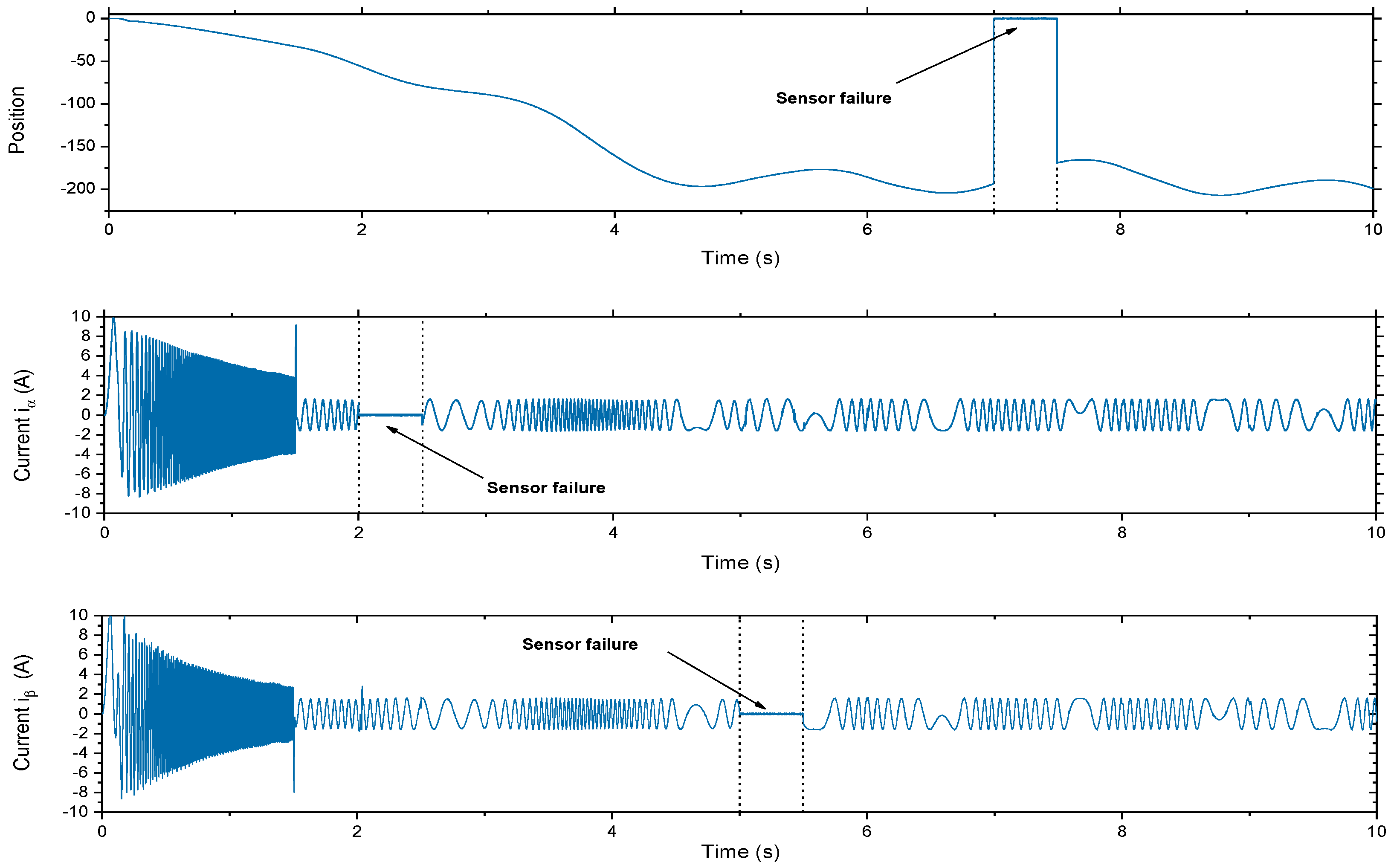
Figure 6 illustrates the behavior of the currents $\alpha$ and $\beta$, as well as the position of the closed-loop system. Different faults are applied to the signals from the current sensors $i_{\alpha }$, $i_{\beta }$ and the position sensor $\theta$, as can be seen in the same figure.

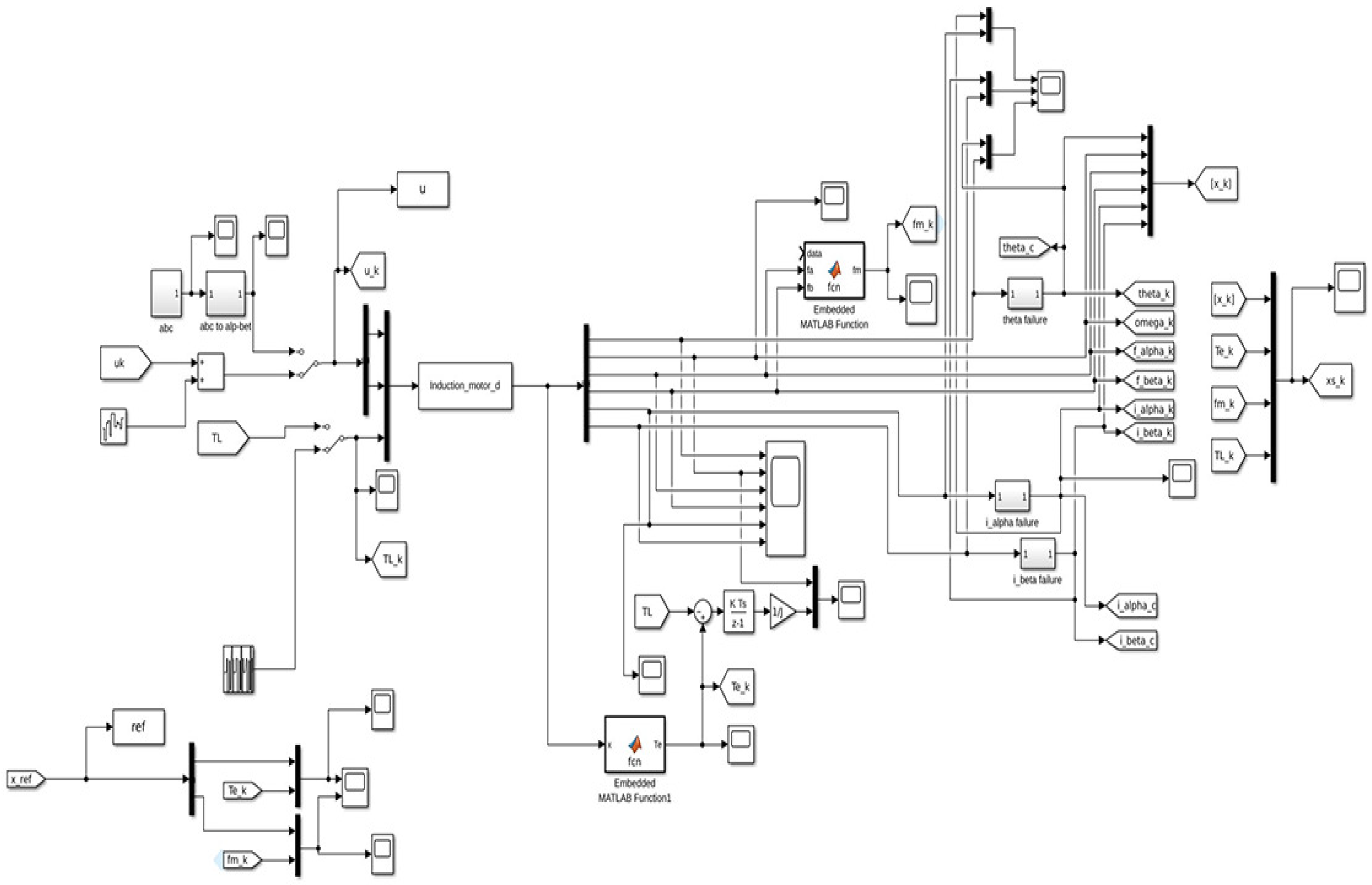
The data presented above were obtained from the Simulink diagram shown in Figure 7. The Simulink model represents a rotational induction motor. The model includes blocks used to simulate fault conditions that may occur in the sensors due to disconnections. Faults are synthetically introduced in the sensors $\theta$ and the current components $i_{\alpha }$ and $i_{\beta }$, which are essential to control and monitor the motor’s performance.

Three faults are introduced, one for each of the sensors mentioned above. The first fault occurs in the current component $i_{\alpha }$ at $t=2$ s. This introduces an interruption in one of the key current measurements that drive the motor dynamics. At $t=5$ s, the second fault appears in the component $i_{\beta }$ affecting the other current measurement. Finally, at $t=7$ s, a fault is introduced in the rotor position ($\theta$). The progressive nature of these faults allows for a step-by-step investigation of the engine’s ability to maintain functionality and performance despite these faults. This setup provides a test environment to simulate real-world engine failure scenarios and allows for the evaluation of fault detection and diagnostic methods, as well as fault-tolerant controllers under controlled conditions.

7.5. Evaluation Criteria

The performance of the neural classifiers was then evaluated using the following evaluation criteria.

Classification accuracy (A) measures the proportion of correct predictions relative to the total number of samples and is calculated as follows:

$$A={\displaystyle \frac{T_P+F_P}{T_P+T_N+F_P+F_N}}$$

(36)

The precision (P) metric evaluates how effective the classification of true positives is compared to false positives:

$$P={\displaystyle \frac{T_P}{T_P+F_P}}$$

(37)

Recall (R) provides information about the proportion of correctly identified positive cases:

$$R={\displaystyle \frac{T_P}{T_P+F_N}}$$

(38)

Finally, the F1 score combines the precision and recall metrics into a single value, which is especially useful when the class distribution is unbalanced:

$$F1=2\ast {\displaystyle \frac{P\ast R}{P+R}}$$

(39)

where $T_P,F_P,T_N,F_N$, are true positive, false positive, true negative, and false negative, respectively.

The ROC curve is a widely used criterion to evaluate the discrimination capacity of classification methods, showing the relationship between the rate of true positives and false positives according to different thresholds. In this curve, a diagonal line indicates random classification performance. The most effective classification methods are those whose curve approaches the upper left edge, indicating high performance. The ability of a model to differentiate between classes is summarized in the area under the curve (AUC); the higher the AUC, the better the classifier’s performance [42].

7.6. Fault-Tolerant Control and Fault-Detection Results

The classification results of the proposed classification methods on the different sensors are presented in

Table 1. Classification results obtained by the MLP and CNN neural classifiers.

Neural Network	Sensor	Accuracy	AUC	Precision	Recall	F1 Score	Execution Time
MLP	Position	0.9914	0.9949	0.9269	0.9949	0.9597
	Current $i_{\alpha }$	0.9539	0.9750	0.7601	0.9750	0.8542	1.67647 × 10−9 s.
	Current $i_{\beta }$	0.9560	0.9765	0.7659	0.9765	0.8585
CNN	Postion	0.9914	0.9955	0.9269	0.9955	0.9610
	Current $i_{\alpha }$	0.9653	0.9809	0.7951	0.9809	0.8783	4.6236 × 10−8 s.
	Current $i_{\beta }$	0.9688	0.9828	0.8080	0.9828	0.8869

. The MLP neural network shows good results, achieving a CA of between 95% and 99% for the evaluated sensors. Regarding the ROC curve, the area under the curve (AUC) varies between 97% and 99%. However, the precision criterion indicates that the MLP neural network makes errors in the classification of true positives, this could be an indicator of acceptable, although not optimal, performance in this metric. On the other hand, the recall value shows that the MLP neural network is capable of correctly classifying false positives, reaching values between 97% and 99%, so the performance in this aspect is acceptable. In the case of the F1 score, which combines precision and recall, it confirms a solid performance of the MLP overall. It is important to note that all samples were classified online without any preprocessing of the data.

On the other hand, the CNN shows higher performance in the evaluation criteria according to the CA; CNN achieves results between 96% and 99%, while the area under the curve (AUC) is between 98% and 99%. The case of precision shows values ranging from 79% to 92%, indicating an acceptable classification of true positives compared to false positives. According to recall, CNN obtains consistent results between 98% and 99%, so CNN has the ability to correctly identify positive cases. Finally, the F1 score is in a range of 88% to 96%, demonstrating an effective balance between precision and recall. In general, CNN outperforms MLP in fault classification and its greater ability to handle complex and non-linear data.

It is noteworthy that the data used for online classification are completely different from those used during the training of deep neural networks. Despite this, the results obtained by both neural classifiers show robust and reliable performance.

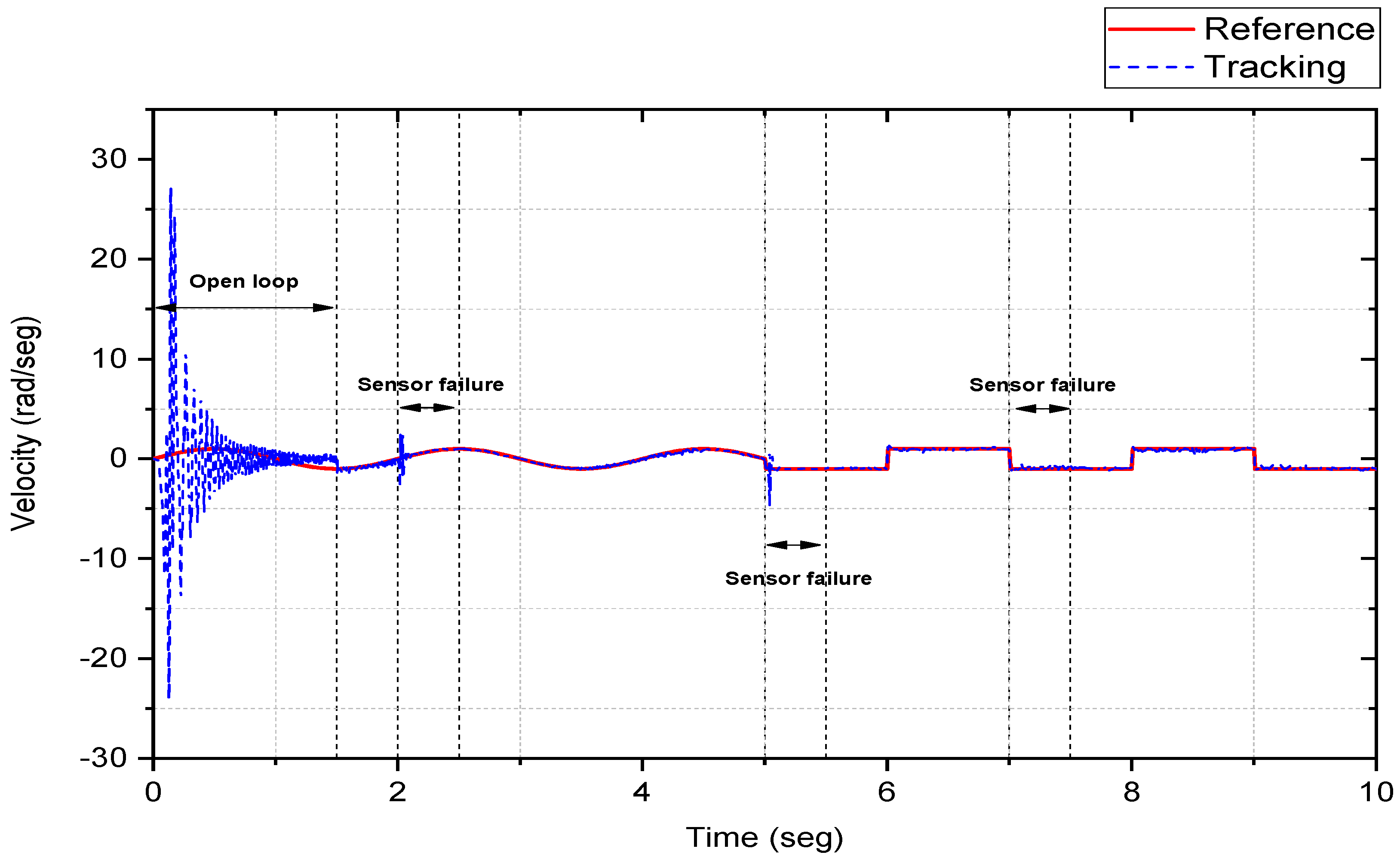
The objective is to achieve the tracking of the stator power reference; for this simulation, a time-varying reference is used. The neural controller was subjected to three different faults that occurred in the three sensors throughout the simulation. The fault events are shown in Figure 8 and are described as follows.

At time $t=2$ s, the current sensor $i_{\alpha }$ presents a fault. Then, the neural classifier immediately detects and isolates the fault, which generates an alert that is provided to the controller. In this event, the neural identifier compensates for the disturbance generated by the fault. Although the fault temporarily alters the motor’s performance, the neural sliding mode fault-tolerant controller has the ability to reject the disturbance and restore system stability in a short period of time.

Then, another failure occurs in the current sensor $i_{\beta }$ at time $t=5$ s; in the same way, the neural classifier has the ability to detect the failure, and this time, the motor control performance is affected to a lesser extent than for the first failure. Thus, despite the disturbance caused by the sensor failure, the stability remains stable despite the failure of the sensor $i_{\beta }$.

Finally, the last fault occurs at time $t=7$ in the position sensor. After the fault identification, the controller takes action to reduce the problems caused by the fault. In fact, the fault does not have a major impact on the reference track; the performance is kept almost unchanged, which demonstrates the controller’s ability to efficiently manage this type of event without compromising the stability or accuracy of the system.

8. Discussion

Overall, the results obtained from the neural sliding mode’s fault-tolerant controller and the neural classifier show robust performance in maintaining engine performance even in the presence of sensor failures.

The neural classifier, based on deep neural networks, was able to accurately differentiate between the different classes (the fault state or the normal state). This allowed the classifier to provide the necessary information to both the controller and the neural identifier, facilitating the compensation of the effects caused by each detected fault.

Furthermore, it can be noted that although the first fault produces a slight disturbance in the system, it manages to stabilize quickly. Under the presence of the second fault, the impact is drastically reduced. Finally, the effect is practically reduced to zero when the third sensor failure occurs. The results show the ability of the neural controller to adapt and effectively mitigate the effects of sensor failures as they occur, thus maintaining system stability and performance over time.

The proposed method stands out from other fault detection approaches due to its accuracy (96–99%), low sensitivity to noise, and a response time of 1.67647 ns, and it does not require a nominal model of the system for its implementation. Unlike methods such as the state observer and Kalman Filters, which are effective for monitoring but require a model and are not currently used in closed-loop control tasks, the proposed method is suitable for both real-time detection and applications in closed-loop control systems. This makes it versatile and efficient in environments where immediate response and accuracy in fault identification are needed, overcoming the limitations of traditional methods that often rely on specific models or are too sensitive to noise. A summary of the comparison is added in

Table 2. Incorporation of methods in the fault-detection literature and the proposed method.

Method	Required Model	Noise Sensitivity	Response Time	Real-Time Detection	Accuracy	Application in Control Tasks	Citations
Deep Neural Network	No (free model)	High	<100 ms	Yes	>99%	Not directly (in monitoring)	[43]
Artificial neural networks	No (free model)	Moderate	28 μs	Yes	94.73% unprocessed, 98.43% processed	Not directly (in monitoring)	[44]
State Observer Approach	Yes	High	Not specified	Yes	High (Not specified)	With potential use	[45]
Kalman Filter/EKF	Yes	High	Not specified	Yes	80–95%	Not directly (in monitoring)	[46]
Redundancy Analysis	No	High	Not specified	Yes	80–97%	Not directly (in monitoring)	[47]
Signal Parity Methods	Yes	High	Not specified	Yes	Effective in diagnosis and isolation	Not directly (in monitoring)	[48]
Fuzzy Logic	No (requires rules)	High	Not specified	Yes	High (based on defuzzification)	Not directly (in monitoring)	[49]
Observer-Based Approach	Yes	High	Not specified	Yes	High (accurate fault determination)	Yes, with fault compensation	[6]
Filter-Based	Yes	High	Not specified (high computational cost)	Yes	High (in well-defined systems)	Not directly (in diagnosis)	[7]
Model-based approach	Yes	Moderate	Not specified	Yes	High in well-defined networks	Not directly (in diagnosis)	[8]
Proposed Method	No	Low	1.67647 × 10−9 s	Yes	96–99%	Applied in closed loop with a controller

.

9. Conclusions

In this study, an online fault-tolerant control scheme was proposed that does not depend on a nominal model of the system. A high-order recurrent neural network (RHONN) trained using the Extended Kalman Filter (EKF) was used to identify the behavior of an induction motor. The identification generated a nonlinear model that allowed the synthesis of a sensor fault-tolerant controller with neural sliding mode, capable of maintaining system stability and minimizing the effects of successive sensor failures, thus achieving a small tracking error. It is important to note that the proposed methodology inserted three faults in different sensors, which were effectively absorbed and compensated by the RHONN model.

Additionally, a neural classifier was implemented to detect and isolate the online faults. Two types of deep neural networks were used, thus demonstrating the potential of deep learning in detecting sensor faults without the need for a nominal model of the system. Typically, in fault-tolerant control schemes, fault detection and isolation are performed by observers comparing the sensor output to continuous estimates. However, these methods rely heavily on nominal models, which are not always easy to obtain and can become inaccurate when system parameters change over time.

For example, methods such as the Luenberger State Observer are based on a mathematical model of the system to estimate its state and detect deviations that could indicate a failure. The Kalman Filter is also popular in fault detection, but this method assumes linearity in the system, which can limit its adaptability and accuracy in complex systems. Other techniques use Analytical Redundancy Analysis, which compares redundant signals in the system to identify discrepancies that could indicate failures. Although it is a useful technique in systems where redundancy is easy to implement, it is inefficient when faced with multiple failures and presents problems in systems without redundant sensors.

Deep neural networks have drawbacks in real-time fault detection, including processing time when the neural network contains too many hidden layers, or the need for large amounts of labeled data to achieve adequate performance, which can be a challenge in problems where data, especially those with faults, are scarce. In this work, these limitations were addressed by proposing improvements in the network structure and optimization to reduce inference times.

The comparative results showed that both deep neural networks were able to classify online with a high level of confidence. The proposed CNN obtained a superior performance in this work. As a future line of research, it is suggested that the use of other specialized time-series neural network architectures, such as long-short-term memory (LSTM) networks, be explored either in their unidirectional or bidirectional (BiLSTM) versions, to further improve fault detection in dynamic environments.