Detection of Damage on Inner and Outer Races of Ball Bearings Using a Low-Cost Monitoring System and Deep Convolution Neural Networks

Abstract

Bearings are vital components in machinery, and their malfunction can result in equipment damage and reduced productivity. As a result, considerable research attention has been directed toward the early detection of bearing faults. With recent rapid advancements in machine learning algorithms, there is increasing interest in proactively diagnosing bearing faults by analyzing signals obtained from bearings. Although numerous studies have introduced machine learning methods for bearing fault diagnosis, the high costs associated with sensors and data acquisition devices limit their practical application in industrial environments. Additionally, research aimed at identifying the root causes of faults through diagnostic algorithms has progressed relatively slowly. This study proposes a cost-effective monitoring system to improve economic feasibility. Its primary benefits include significant cost savings compared to traditional high-priced equipment, along with versatility and ease of installation, enabling straightforward attachment and removal. The system collects data by measuring the vibrations of both normal and faulty bearings under various operating conditions on a test bed. Using these data, a deep neural network is trained to enable real-time feature extraction and classification of bearing conditions. Furthermore, an explainable AI technique is applied to extract key feature values identified by the fault classification algorithm, providing a method to support the analysis of fault causes.

1. Introduction

Bearings are vital mechanical elements that support rotating shafts with minimal friction, ensuring the smooth functioning of machinery. They are extensively utilized in a variety of mechanical systems, especially in intricate and critical applications such as induction motors, automobiles, aircraft, and industrial machinery [1,2]. However, when bearings become damaged or fail, they can disrupt machine operations or even cause complete system shutdowns, leading to expensive repairs and significant losses in productivity. In fact, bearing problems are responsible for more than 40% of induction motor failures [3,4]. According to catalogs provided by major bearing manufacturers [5,6,7], the causes of bearing failure include fatigue, insufficient lubrication, contamination, overloading, improper installation, thermal overload, and misalignment. These factors lead to wear on the key mechanical components within the bearing, such as the inner and outer races and the balls. While bearing failures can occur due to factors beyond mechanical elements, typically, severe wear on the mechanical components of the bearing results in its failure. Consequently, it is essential to continuously monitor the condition of bearings and detect any damage or anomalies at an early stage. By identifying potential issues before they escalate into severe damage, preventive actions can be taken to ensure stable machine operations. Early detection not only lowers maintenance costs but also maximizes machine uptime. Utilizing predictive maintenance technologies and diagnostic tools to anticipate bearing damage can effectively prevent unexpected breakdowns and the associated substantial financial losses [8,9,10].

To address this need, recent research has explored condition monitoring techniques, including vibration spectrum analysis, sound waveform analysis, and temperature analysis, to detect rolling bearing damage. In industry, SKF has proposed the Proactive Reliability Maintenance (PRM) program, which offers a service to predict and address various potential failures in bearings within mechanical systems in advance. This service detects signals such as vibrations and temperatures generated by the system and uses them to identify issues with the bearings [11]. However, this approach has not yet encompassed signal analysis through machine learning and the identification of the underlying causes of these problems. In academia, Tahmasbi et al. diagnosed bearing failures and performed root cause analysis through vibration investigations on a 2300 kW motor, identifying resonance and inadequate lubrication as key failure causes and implementing corrective actions that improved the time between failures from 3 to 11 months [12]. Jakobson et al. presented a method for detecting insufficient lubrication in rolling bearings using a low-cost MEMS ultrasonic microphone, where vibration signals are analyzed under varying lubrication conditions and the viscosity ratio of the lubricant serves as a metric for oil-film quality, with results compared to predictions from regression and neural network models [13]. Fang et al. suggested a method that integrates autocorrelation with wavelet transform and cyclostationary theory to effectively identify compound faults in rolling bearings of aeroengines, outperforming conventional methods in fault separation and detection regardless of sensor orientation [14]. Xu et al. developed a digital twin-empowered discriminative graph learning network (DT-DGLN) for rolling bearing fault diagnosis using unlabeled industrial data, addressing the challenge of limited datasets by creating a detailed digital twin model and a framework that adapts knowledge from simulated to real signals for efficient fault recognition [15]. Gunerkar et al. introduced a novel bearing fault diagnosis method that integrates vibration and acoustic emission sensors through data acquisition, signal processing, feature extraction, K-nearest neighbor classification, high-level data fusion, and decision-making steps, enabling the early detection of all rolling bearing faults by leveraging the unique strengths of each sensor type [16]. Wang et al. used acoustic emissions and various sensing techniques to monitor and correlate wear mechanisms in oil-lubricated metal sliding contacts at the micro-scale [17]. Chen et al. demonstrated that combining online vibration and electrostatic sensors with advanced data fusion techniques effectively detects bearing deterioration before failure and enhances anomaly detection by identifying key diagnostic variables [18]. Yang et al. studied vibration characteristics resulting from cage damage by recording vibration and temperature data across the entire life cycle of two types of deep groove ball bearings (6210 and 6011) under abnormal load conditions [19]. Additionally, Küçükoglu Dogan et al. evaluated the fault detection and lifespan of polymer hybrid ball bearings using both an accelerometer and load cell under varying load conditions, showing that these sensors can provide complementary insights for bearing condition monitoring [20]. Zhang et al. synthesized CdTe/ZnS-SiO₂ nanocomposites to enhance the thermal stability and photoluminescence of CdTe quantum dots, enabling their effective use as reversible temperature sensors for thermal monitoring of bearing components in high-speed applications [21]. However, challenges remain in implementing these monitoring systems in industrial settings, primarily due to the high costs and limited integration capabilities of these systems.

With advances in machine learning algorithms, recent research has increasingly applied machine learning models to nonlinear and complex physical systems for bearing fault diagnosis. Magadán et al. predicted the remaining useful life of electric motor bearings using a Stacked Variational Denoising Autoencoder (SVDAE) and Bidirectional Long Short-Term Memory (BiLSTM) network [22]. Ma et al. proposed an ensemble deep learning diagnosis method that integrates a Convolution Residual Network (CRN), Deep Belief Network (DBN), and Deep Auto-Encoder (DAE) through a multi-objective optimization strategy, improving the diagnosis of rotor and bearing faults in rotating machinery compared to traditional models [23]. Elforjani et al. applied three supervised machine learning techniques—support vector machine regression, multilayer artificial neural networks, and Gaussian process regression—to correlate acoustic emission features with the natural wear of slow-speed bearings, concluding that neural networks can effectively estimate the remaining useful life of components using appropriate data and structure [24]. Hao et al. used a 1D Convolutional Long Short-Term Memory (1D CNN-LSTM) network to diagnose bearing conditions from vibration signals captured by multiple sensors [25]. Zhang et al. investigated a new deep learning model for intelligent fault diagnosis that effectively operates in noisy environments and adapts to changing working loads without requiring time-consuming denoising preprocessing or domain adaptation algorithms, achieving high accuracy and providing insights into its performance through feature visualization [26]. Yu et al. proposed a novel feature extraction method for improving bearing fault diagnosis accuracy by utilizing empirical mode decomposition and combining K-means clustering with standard deviation for selecting sensitive characteristics, along with a modified dimensionality reduction approach, ultimately demonstrating effective performance across 12 bearing fault conditions [27]. Feng Jia et al. utilized deep neural networks (DNNs) for intelligent fault diagnosis in rotating machinery by analyzing large-scale vibration data from AE sensors [28]. Guo et al. proposed a novel hierarchical learning-rate-adaptive deep convolutional neural network for accurately diagnosing bearing faults and evaluating their severity, achieving satisfactory results in fault-pattern recognition and fault-size assessment when tested on data from a test rig, outperforming existing methods [29]. While most previous studies have focused on training machine learning models and improving their accuracy and performance, this research presents a method for diagnosing bearing faults using a DNN model and explains the reasons behind fault classification through the use of explainable AI (xAI) techniques.

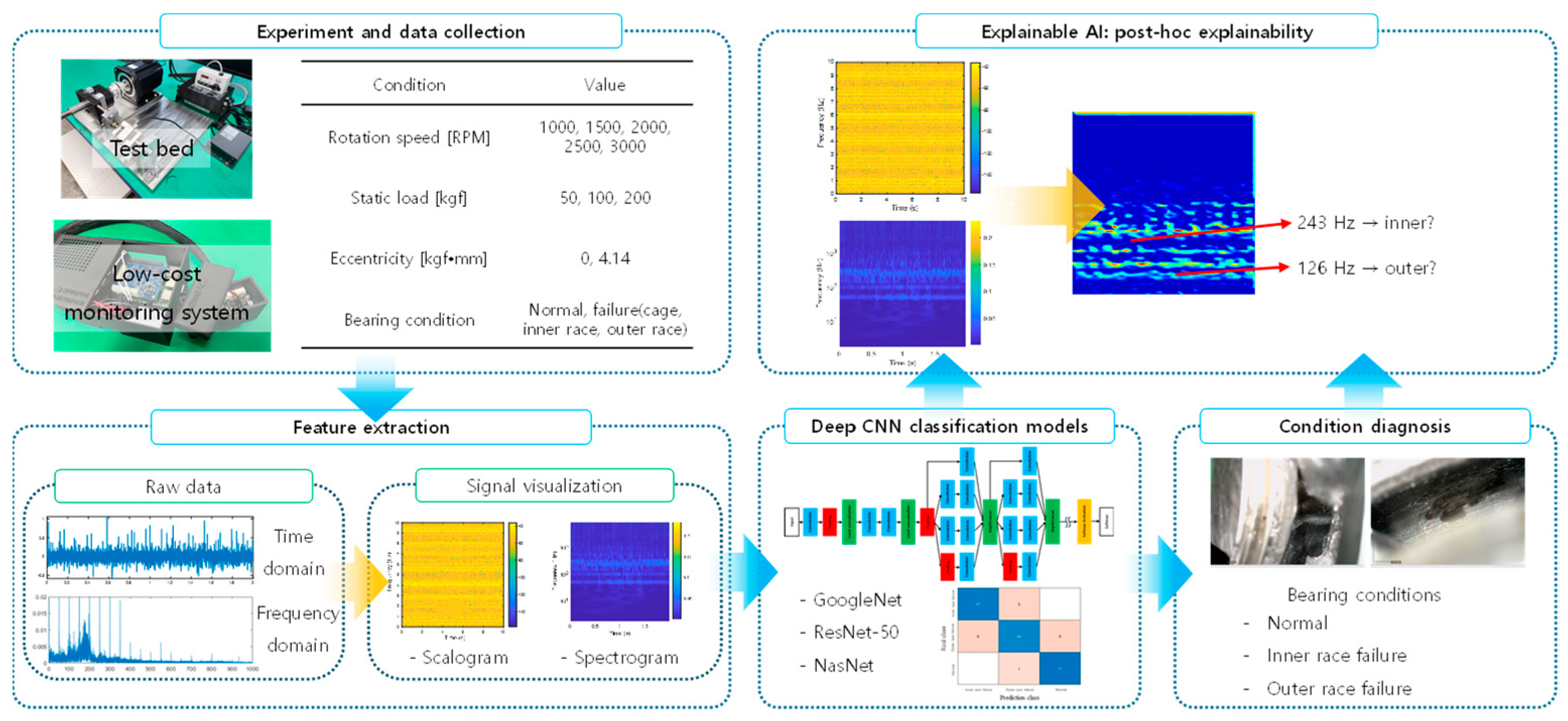
This study developed a cost-effective monitoring system using affordable sensors such as accelerometers, microphones, and piezo sensors, along with a budget-friendly data acquisition (DAQ) system, and validated its reliability against high-end systems. The low-cost monitoring setup was mounted on a test bed, where experiments were conducted under 72 different operating conditions to gather data. The collected data were visualized as scalograms and spectrograms, demonstrating that a deep neural network (DNN) model could accurately classify bearing faults and normal states. Additionally, the study proposed a method for extracting features from the trained DNN model using xAI, which confirmed the reliability of fault cause analysis by comparing the results with theoretical failure frequencies.

2. Experiment Setup and Low-Cost Monitoring System

2.1. Test Bed

A test bed was assembled to generate signals from both functioning and faulty bearings. Illustrated in Figure 1, the setup includes a motor, motor coupler, support bearings, specimen bearings, a rotating shaft, and a load cell. Constructed from S45C steel and weighing roughly 50 kg, the test bed effectively reduces vibrations caused by the motor’s high-speed rotation. It is equipped with a 2 kW BLDC motor that can operate up to 3000 RPM. A deep groove ball bearing is employed as the specimen bearing in both its normal and damaged conditions, while a thrust needle bearing is chosen as the support bearing for its superior radial load safety factor compared to ball bearings, thereby supporting the rotating shaft. The motor is connected to the rotating shaft through a motor coupler.

The test bed is engineered to accommodate both static and dynamic loading conditions. For static loads, a bolt on the right side is tightened, allowing up to 200 kgf of radial static load to be applied using a load cell (CSBA-200L, Curiosity Technology, Paju, Republic of Korea) and an indicator (CTI-2100, Curiosity Technology, Paju, Republic of Korea). To replicate dynamic loads caused by shaft eccentricity, a 25.4 g bolt is attached to the eccentric element illustrated in Figure 1. The attachment points, labeled A, B, and C, are positioned at distances of 95.3 mm, 77.8 mm, and 55 mm from the central axis, respectively, creating eccentricity levels of 1×, 2×, and 3×.

2.2. Low-Cost Monitoring System

The low-cost monitoring system is composed of two main components: a sensor module and a data acquisition module. The sensor module, which includes an accelerometer, a microphone, and a piezo disc, is mounted on top of the specimen bearing. The data acquisition module consists of a Raspberry Pi 4B paired with a DAQ HAT. Specifically, the DFR 0143 accelerometer is a three-axis device having adjustable sensitivity settings of 1.5 g and 6 g, yielding output voltages of approximately 800 mV/g and 220 mV/g, respectively. The MAX 9814 microphone is equipped with automatic gain control, allowing it to effectively adapt to varying noise levels, which is particularly useful in environments with significant motor noise. For vibration detection, the DFR 0052 piezo disc sensor, measuring 20 mm in diameter, leverages the piezoelectric properties of PZT to achieve high sensitivity to voltage fluctuations caused by vibrations. To enhance signal strength, an intermediate material was inserted between the PLA module and the PZT, with aluminum selected for the low-cost module due to its ability to produce peak amplitudes two to three times greater than glassfiber-reinforced polyamide.

Figure 2a illustrates the sensor and DAQ modules, highlighting the Raspberry Pi 4B’s role as the data acquisition unit. Although the Raspberry Pi 4B has a maximum sampling rate of 3.3 kHz, the addition of an MCC128 DAQ HAT enables data collection at up to 20 kHz. Figure 2b,c show the arrangement of components within both the sensor and data acquisition modules. The MCC128 from Measurement Computing’s DAQ series offers a 16-bit resolution and supports either eight single-ended or four differential analog input channels. In this setup, the three-axis accelerometer, piezo disc sensor, and microphone are connected to five single-ended input channels on the MCC128. Data gathered by the collection module can be accessed from a PC through a shared gateway and are processed in real time.

The sensor module is affixed to the top of the specimen bearing holder within the test bed. Its design is more compact than the specimen bearing holder, allowing it to be securely attached and easily removed using neodymium magnets. To ensure robust attachment, neodymium magnets were selected for their strong holding power. Additionally, the sensor cables are shielded to prevent interference from external noise. During the experiments with the sensor module attached, no changes in sensor position were observed due to a decrease in the magnetic force of the magnets. When the motor in the test bed operates, the sensor module captures the noise and vibrations produced by the specimen bearing and transmits these signals to the DAQ module. Furthermore, the housings made of ABS plastic for both the sensor module and the DAQ module are 3D printed to provide protection against external shocks and contamination, ensuring the durability and reliability of the monitoring system.

2.3. Validation of Low-Cost Monitoring System

A comparative study was conducted to evaluate the reliability of the low-cost sensor module for bearing diagnosis in comparison to high-cost industrial sensors. The components used for this validation are detailed in

Table 1. Parts list of low- and high-cost monitoring systems.

Type	High-Cost Sensor	Low-Cost Sensor
DAQ	NI cDAQ 9174	Raspberry Pi 4GB
ADC	NI 9775	DAQ HAT MCC 128
AE and Piezo Disc	Physical Acoustics R15	DFR0052
Accelerometer	CTC AC214-1D	MMA7361 DFR0143
Mic	Crysound 333-T1	MAX9814

. While high-cost sensors are established and dependable products within the industry, their low-cost counterparts are available for approximately 2% of the price, as listed in

Table 2. Price comparison between the low- and high-cost monitoring systems.

Low-Cost Monitoring System Components	Price	High-Cost Monitoring System Components	Price	Price Comparison (%)
PZT sensor (DFR 0052)	$7	AE sensor (R15a)	$4500	0.2%
Acc sensor (DFR 0143)	$11	Acc sensor (AC214)	$600	1.8%
Microphone (MAX 9814)	$10	Microphone (T333)	$800	1.3%
Raspberry Pi 4B	$80	DAQ (NI-9775 and -9174)	$6000	6.3%
MCC128 (DAQ HAT)	$300

. Additionally, the low-cost data acquisition (DAQ) module was selected, costing less than 5% of the high-cost DAQ used for validation. Consequently, the proposed low-cost monitoring system can be implemented at roughly 3% of the cost of a system comprising high-cost sensors and DAQ.

To verify the reliability of the low-cost monitoring system, a series of experiments was performed, divided into two parts: comparing the high-cost DAQ with the low-cost DAQ, and comparing the low-cost sensors with the high-cost sensors. Initially, both low-cost and high-cost sensors were connected to a high-end data acquisition device (cDAQ 9174, NI) and tested under the conditions specified in Table 2. The results, summarized in Figure 3, indicate that the low-cost accelerometer exhibited similar trends to the high-cost accelerometer at frequencies below 1 kHz.

Figure 3 compares the frequency-dependent sensitivities of high-cost sensors and low-cost sensors. To facilitate a comparison of the graph shapes, the data acquired by each sensor were scaled by a factor of 10 for the low-cost accelerometer, 2 for the high-cost microphone signal, and 8 for the low-cost piezo sensor. Taking these scaling factors into account, the low-cost accelerometer exhibits approximately 10 times lower sensitivity compared to the high-cost sensor. For the low-cost piezo sensor, the waveform shape differs, making a perfect comparison challenging. However, it appears to be about 20 times less sensitive in the 5–10 kHz range. In contrast, within the 100–500 Hz range, the low-cost piezo sensor shows sensitivities up to more than 20 times higher than the high-cost sensor. Regarding microphones, the low-cost sensor demonstrates 2–4 times higher sensitivity per frequency compared to the high-cost sensor. This increased sensitivity is likely due to the high-cost microphone sensor being positioned farther from the specimen bearing than the low-cost sensor.

In the case of accelerometers, both sensors display similar frequency patterns around 50–400 Hz. However, beyond 400 Hz, the low-cost accelerometer appears to produce stronger signals. Additionally, the low-cost sensor was unable to measure frequencies above 1000 Hz, resulting in the inability to acquire data observable by the high-cost sensor. These findings indicate that while the sensitivity below 400 Hz is somewhat reduced when using the low-cost accelerometer, it can still capture the same frequency patterns as the high-cost sensor.

For microphone sensors, the low-cost sensor was found to have sensitivities approximately 2–4 times higher than the high-cost sensor. Considering the reliability of the high-cost sensor, the low-cost sensor has the drawback of being unable to capture signals around the 80–100 Hz frequency range. Moreover, at frequencies above 5000 Hz, the sensitivity of the low-cost sensor decreases compared to the high-cost sensor. Although the frequency patterns differ in certain ranges compared to the high-cost sensor, overall, it was demonstrated that the low-cost sensor can also capture signals within the frequency range measured by the high-cost sensor.

Finally, the low-cost piezo sensor did not exhibit high sensitivity above 5000 Hz, unlike the high-cost AE sensor. However, the low-cost sensor was more sensitive to vibrations above 1000 Hz within the 100–1000 Hz range. This suggests that while the high-cost AE sensor is designed to be sensitive to signals above 5000 Hz, the low-cost sensor is configured to be more sensitive around 100–1000 Hz. In the case of bearing failure, fault signals are often observed at frequencies below 1000 Hz, indicating that the sensitivity distribution of the low-cost sensor may be more advantageous than that of the high-cost sensor.

To further validate the reliability of the low-cost DAQ, the DAQ module, consisting of a Raspberry Pi 4B and MCC128, was connected to three low-cost sensors and subjected to experiments under the conditions outlined in

Table 3. Experiment conditions for validating low-cost monitoring system.

Experiment Conditions	Value
Bearing condition	Normal
Rotation speed [RPM]	1750
Static load [kgf]	60
Sampling rate [kHz]	20
Data collection time [s]	10

. Measurements were conducted at a sampling rate of 20 kHz using BNC-to-alligator-clip cables. As shown in Figure 4, the signals acquired by both the high-cost DAQ and the low-cost DAQ were identical across all low-cost sensors except for certain frequency domains. When combining the accelerometer with the high-cost DAQ, a peak occurs around 830 Hz. This peak appears to be detectable by the high-cost DAQ but not by the low-cost DAQ. In other regions, signals were consistently captured by all DAQs. Additionally, different sensitivity characteristics were observed at frequencies below 500 Hz. This indicates that the high-cost DAQ can collect data more sensitively compared to the low-cost DAQ. This demonstrates that the low-cost DAQ module can achieve signal measurement performance comparable to that of the high-cost DAQ.

2.4. Experiments

Experiments for bearing fault diagnosis were performed using the developed test bed and a cost-effective monitoring system to gather necessary data as listed in

Table 4. Experiment conditions for validating low-cost monitoring system.

Experiment Conditions	Value
Bearing condition	Normal, inner race failure, and outer race failure
Rotation speed [RPM]	1000, 1500, 2000, 2500, and 3000
Static load [kgf]	50, 100, and 200
Eccentricity [kgf∙mm]	0, 4.14
Sampling rate [kHz]	20
Data collection time [s]	10

. A total of 72 distinct conditions were evaluated, with each condition being replicated 10 times. For safety reasons, tests at 2500 RPM and 3000 RPM were not conducted when eccentricity was introduced. To reduce assembly errors during the transition from normal to faulty bearings, damage was induced by drilling the inner and outer races of the test bearing, while the bearing designated for collecting normal data remained securely mounted in the bearing holder. Figure 5 illustrates the procedure for creating damage on the surfaces of the inner and outer races using a drill. The induced damage was randomly generated to replicate wear or failure conditions. Through these rotational bearing experiments, as depicted in Figure 6, a total of 720 samples were obtained, resulting in 2160 time-series data points collected from three sensors.

3. Bearing Fault Diagnosis via DNN

The process of bearing fault diagnosis is essential for maintaining the safety and efficiency of machinery. This procedure is structured into several key stages, beginning with the collection of monitoring data. Real-time data are acquired through an economical monitoring system equipped with three sensors, each possessing distinct characteristics and sensitivities, thereby enabling comprehensive data acquisition. The collected data then undergo a signal processing phase, where noise is eliminated and critical information is refined into a more usable form. Analysis revealed that measurements above 1 kHz did not provide meaningful features for differentiating between faulty and normal signals and were susceptible to external noise. Consequently, a cutoff frequency of 1 kHz was implemented for all sensors, effectively removing high-frequency components.

Following signal preprocessing, the data advance to the visualization stage, where they are transformed into graphical representations such as spectrograms and scalograms to facilitate the interpretation of data characteristics. A spectrogram typically employs the Fourier transform to convert the signal into the frequency domain, analyzing short segments of the signal to identify frequency components over time. In contrast, a scalogram utilizes the wavelet transform to temporally localize frequency components, capturing changes in specific frequency bands with higher resolution. This makes the scalogram particularly advantageous for analyzing the frequency components of non-stationary signals, thereby complementing the information provided by spectrograms. The visualization process generates a total of 4320 images, which are subsequently used to train deep neural network (DNN) models. Detailed descriptions of these processes are illustrated in Figure 7.

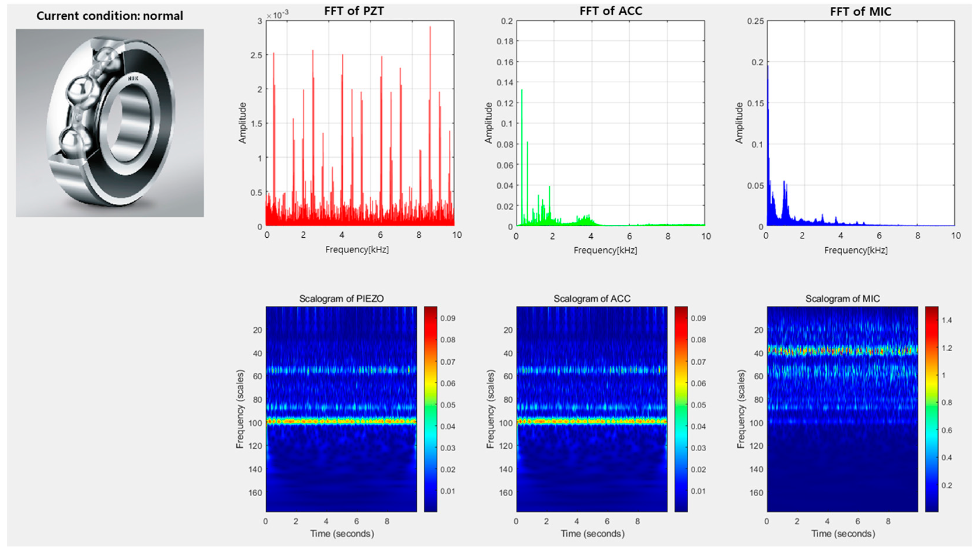
In the fault diagnosis phase, the integration of data collected simultaneously from the three sensors is crucial for combining the prediction results of each model. To achieve this, a majority voting method, also known as an ensemble technique, is employed to merge the predictions from multiple models, ultimately determining the bearing condition. The data from the three sensors is visualized and utilized to train the DNN models to classify bearings as either normal or faulty. Each classification outcome is determined by the majority vote, effectively reflecting the characteristics extracted from the visualized data of each sensor. 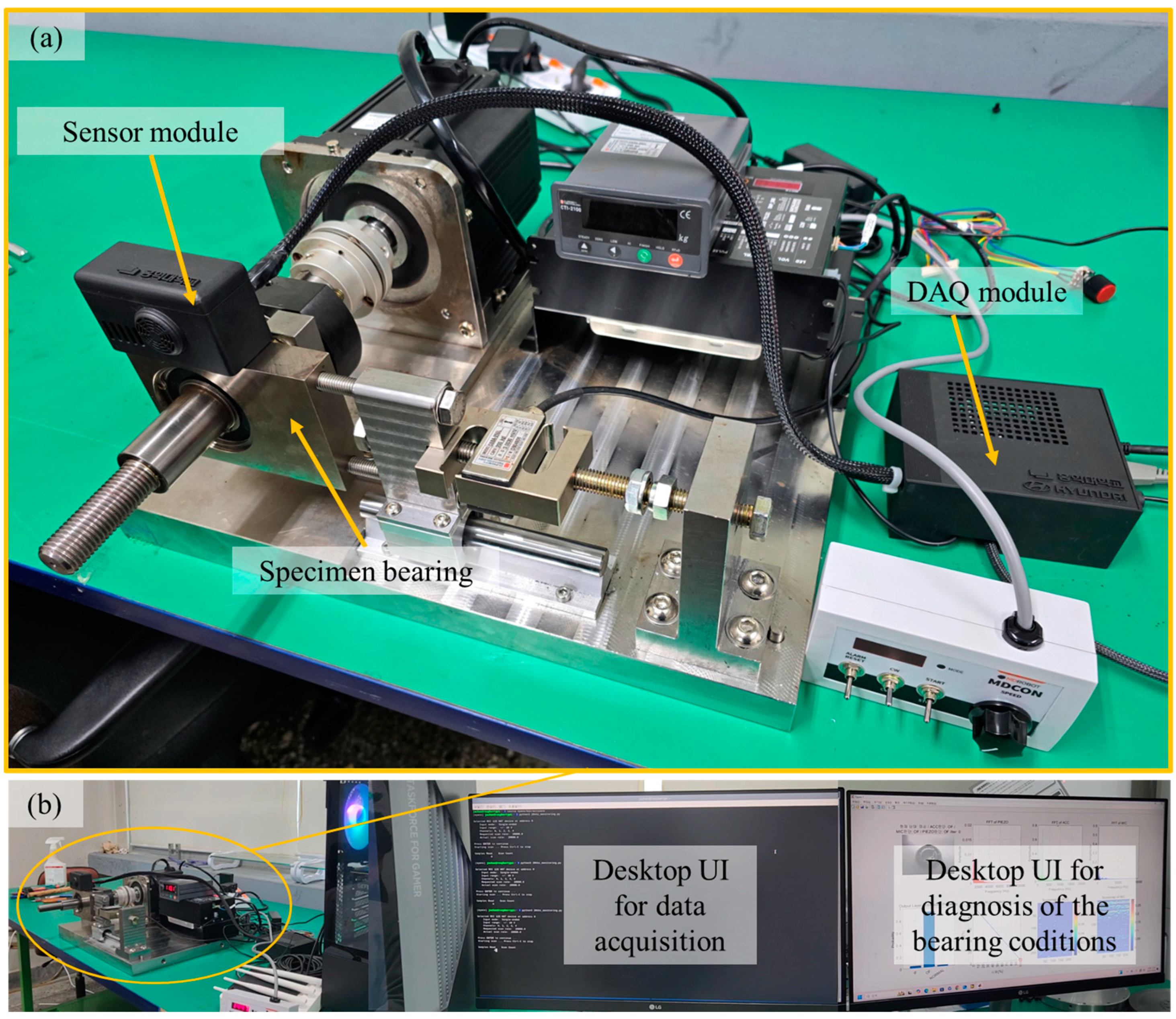As depicted in Figure 8, the user interface is designed to facilitate easy access to bearing condition diagnosis results by inputting new real-time data from the low-cost monitoring system into the trained DNN models. Additionally, various types of information, including sensor-specific FFT graphs, scalograms, and cumulative diagnosis counts, are updated and displayed in real-time, providing immediate access to insights regarding bearing analysis.

In this testbed, experiments were conducted under 72 distinct conditions, resulting in the collection of 2160 time-series signals from 10 bearings and 3 sensors. These signals were utilized to train deep neural network (DNN) models, thereby significantly enhancing the accuracy of bearing fault diagnosis. Recognizing that the fast Fourier transform (FFT) alone is limited in capturing the subtle distinctions between normal and faulty bearings, additional data visualization techniques such as spectrograms and scalograms were employed.

The spectrogram was generated using the following procedure. Initially, the signal was segmented into fixed-length frames (windows), and a window function was applied to each segment to minimize boundary effects. Subsequently, a Fourier transform was performed on each windowed frame, converting the signal from the time domain to the frequency domain. This transformation enabled the analysis of the frequency components within each frame, allowing for the extraction of both the magnitude and phase information of these components. The extracted data were then organized over time and visualized in a two-dimensional graphic, with frequency depicted on the Y-axis, time on the X-axis, and amplitude represented through variations in color or brightness.

The scalogram was produced using the following methodology. The signal underwent a wavelet transform, a technique that localizes frequency components in time, enabling high-resolution detection of changes in non-stationary signals. In this study, the Morlet wavelet was utilized. By applying the wavelet transform, the signal was transformed into the time–frequency domain, generating coefficients that depict the variation of frequency components over time. The visualization parameters included a signal length of 199,000 samples, a sampling frequency of 20,000 Hz, and 12 voices per octave. Utilizing these coefficients, the scalogram was created with time represented on the X-axis and frequency on the Y-axis, while the energy of each frequency band was visualized through color or brightness levels. In this visualization process, the intensity of each frequency band was depicted using a color map to represent the strength of the signal.

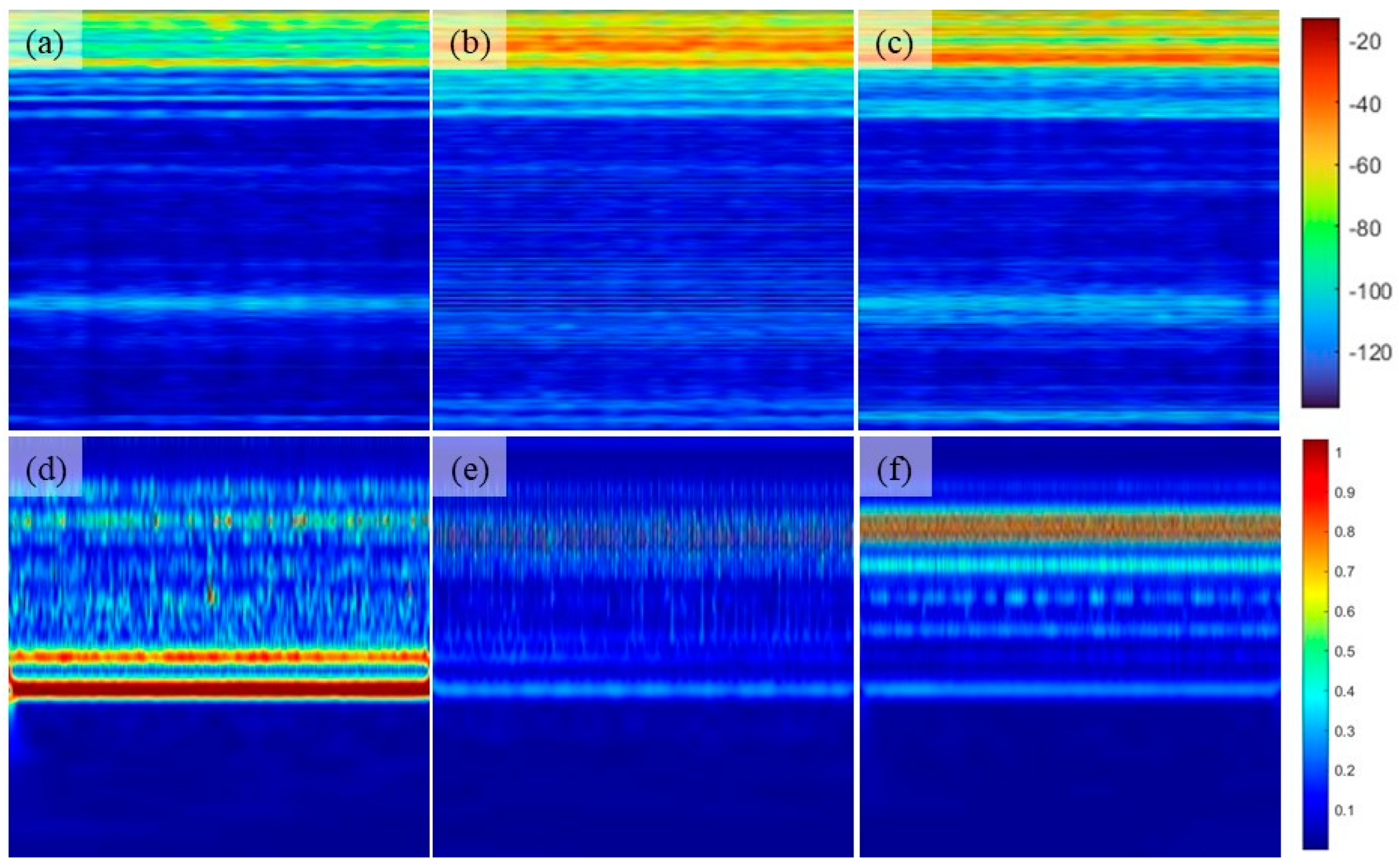
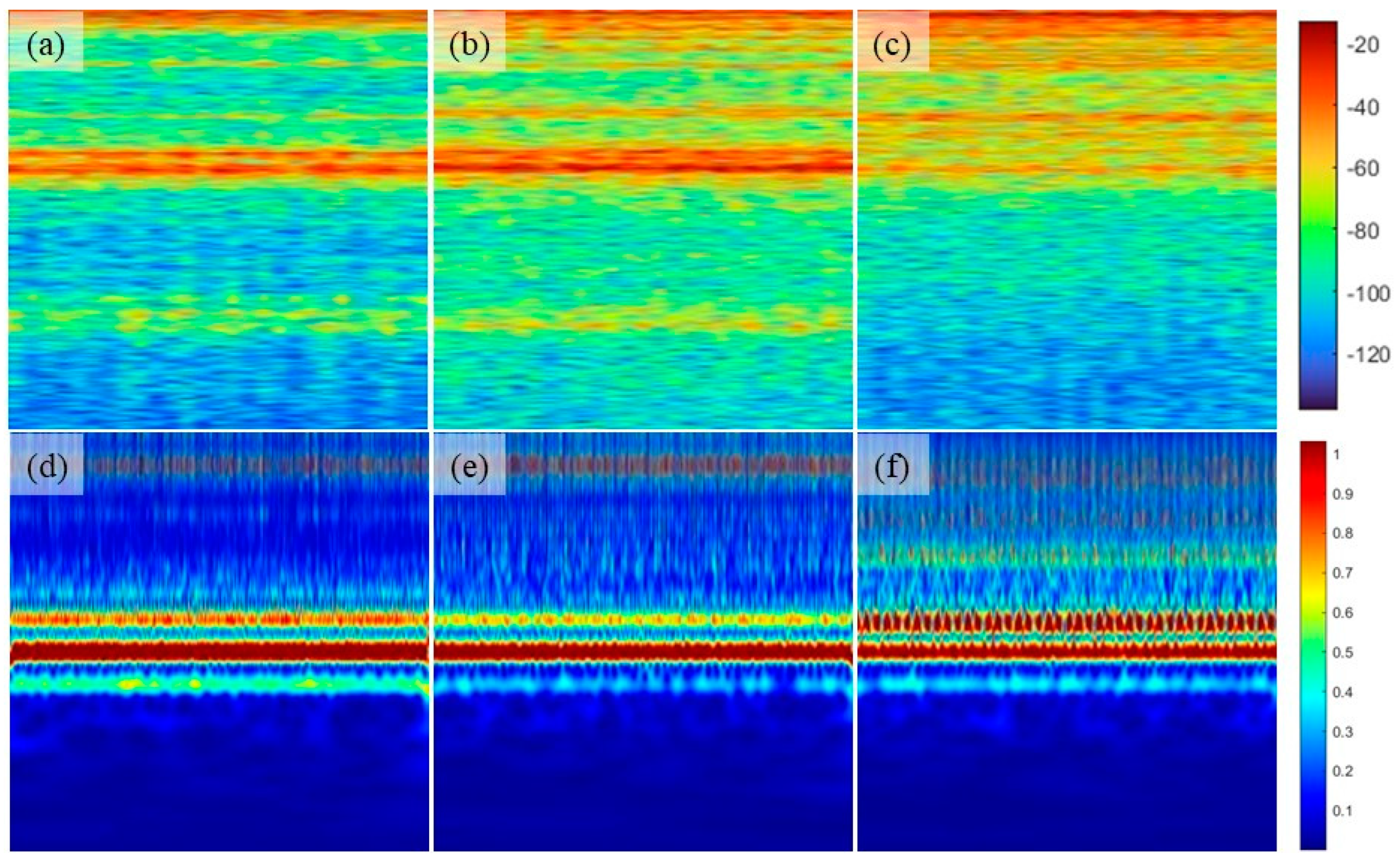
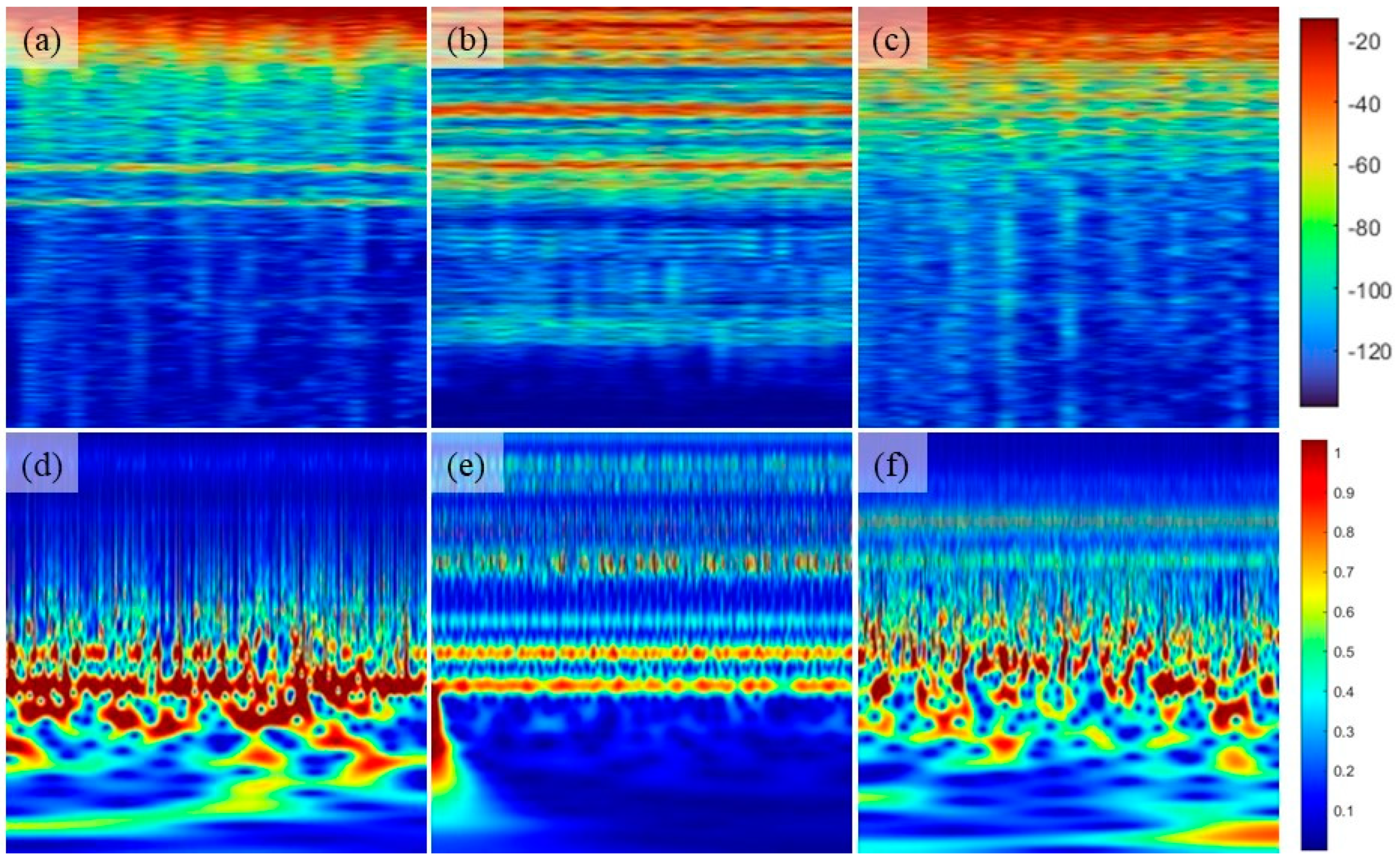
Figure 9, Figure 10 and Figure 11 display scalograms and spectrograms that clearly highlight amplitude variations and irregular patterns in data from faulty bearings over time. Each figure illustrates time-series data collected from the accelerometer, microphone, and piezo sensor, respectively. Across all figures, the scalograms demonstrate a noticeable visual distinction between normal and faulty conditions, a difference that is more pronounced than in the spectrograms. This enhanced distinction is attributed to the scalogram’s capability to analyze non-stationary signals at higher resolution, making anomalies in faulty bearings more evident. Conversely, while the spectrograms do not differentiate as distinctly between normal and faulty states, they do indicate that specific frequency values are significantly elevated in faulty bearings compared to their normal counterparts.

The aim of this study was to develop a model capable of distinguishing between faulty and normal bearings by training deep neural network (DNN) models using spectrogram and scalogram images derived from data visualization. The DNN architectures utilized in this research include GoogLeNet-V1, ResNet-50-V2, and NasNet-Mobile.

GoogLeNet, introduced by Google in 2014, features an innovative architecture centered around the Inception module. This design incorporates multiple kernel sizes (1 × 1, 3 × 3, 5 × 5) within the same layer to capture features at various scales. The network comprises 22 layers, including nine Inception modules, and employs global average pooling instead of fully connected layers at the end to mitigate overfitting. GoogLeNet is recognized for its computational efficiency and relatively low number of parameters, resulting in moderate training times. Its architecture makes it well suited for a wide range of image classification tasks and enables its application in real-time scenarios.

ResNet-50, developed by Microsoft in 2015, is a Residual Network that leverages residual learning to facilitate the training of deeper networks. The “50” in its name indicates the network’s depth, consisting of 50 layers. ResNet-50 utilizes skip connections that preserve the identity across 3 × 3 convolutional layers, allowing gradients to flow effectively without vanishing. This architecture has demonstrated exceptional performance in the ImageNet challenge and supports the training of very deep networks. Despite its depth, ResNet-50 benefits from skip connections that streamline training times relative to its complexity. It is extensively employed in various computer vision tasks requiring deep models, particularly in object detection and segmentation.

NasNet, introduced by Google in 2017, is a Neural Architecture Search Network developed through automated architecture search. It features a sophisticated architecture composed of repeated basic blocks or cells, enabling the model to learn more abstract features. NasNet generally achieves superior performance due to its optimized design, which is the result of automated search processes. However, its intricate architecture and larger number of parameters demand greater computational resources and can lead to longer training durations. Nonetheless, NasNet can be efficiently adapted for mobile applications. Designed for high-performance tasks, NasNet serves as a state-of-the-art model in challenging datasets and competitive environments.

By leveraging these advanced DNN architectures, this study aimed to enhance the accuracy and reliability of bearing fault diagnosis, facilitating early detection and maintenance in industrial applications.

A total of 2160 visualized images representing different bearing states were employed to train the three DNN models, and their classification accuracies were subsequently evaluated.

Table 5. Classification accuracy of the DNN models.

Models	Accuracy	Training Time
GoogLeNet	89.8%	65 s
ResNet-50	89.4%	143 s
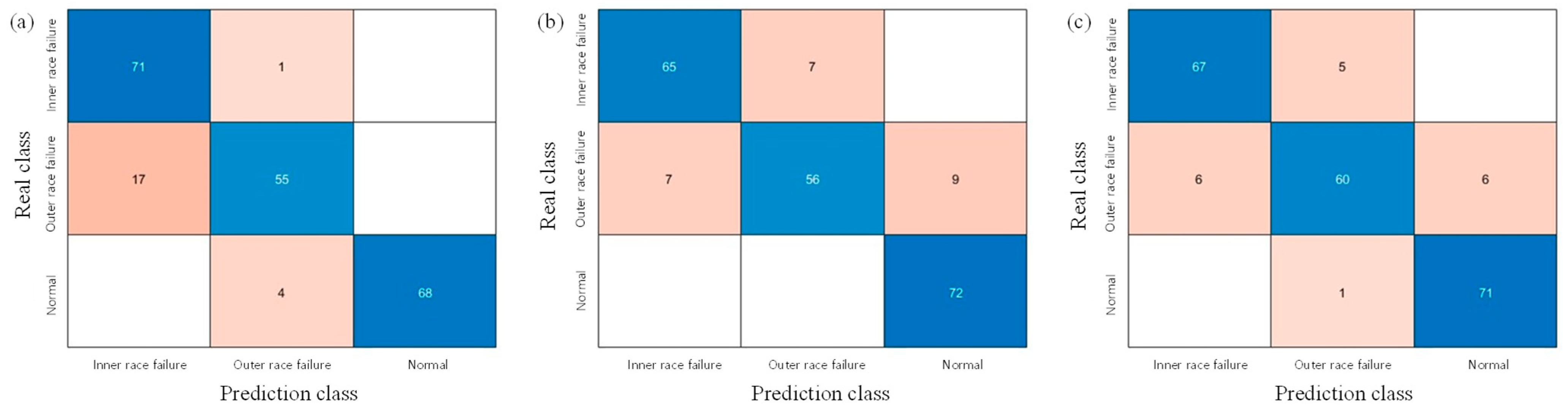
NasNet	91.7%	612 s

provides a summary of the models’ accuracy and training speeds. The overall findings reveal that NasNet achieved the highest classification accuracy in differentiating between normal and faulty states. In contrast, GoogLeNet, with its relatively shallow architecture, demonstrated faster training times. Furthermore, the confusion matrices presented in Figure 12 indicate that GoogLeNet exhibited a higher error rate in distinguishing between inner race and outer race defects compared to the other models. This suggests that GoogLeNet’s shallower structure may limit its ability to effectively extract the features necessary for accurately classifying faults in the inner and outer rings. On the other hand, ResNet-50 showed slightly lower performance in classifying normal versus faulty conditions compared to NasNet and GoogLeNet.

According to the confusion matrices in Figure 12, all models exhibit errors when classifying damages to the outer race and inner race. This suggests that even in damaged states, the waveform differences between the outer and inner races are not significantly greater compared to normal conditions. While the differences between normal rotation and rotation with damage to the outer and inner races can be relatively easily classified using spectrograms or scalograms, it appears difficult to distinguish between damages to the outer and inner races when both are present.

To ensure the reliability of the DNN models in classifying bearing states, an explainable AI (xAI) technique was implemented to identify the features utilized for fault assessment. The xAI approach visually represents the scores predicted by the model for each image’s specific class and generates score maps that display class probabilities for each pixel by mapping scores across multiple classes. These score maps highlight the regions of the image that were most significant during the model’s analysis. Addressing the inherent ‘black box’ nature of DNN models, the xAI functionality facilitates a visual interpretation of the decision-making process, allowing for the assessment of how specific areas of the image influenced the model’s classifications. This functionality was implemented using MATLAB R2024a’s scoremap feature to evaluate the critical points contributing to the model’s decisions.

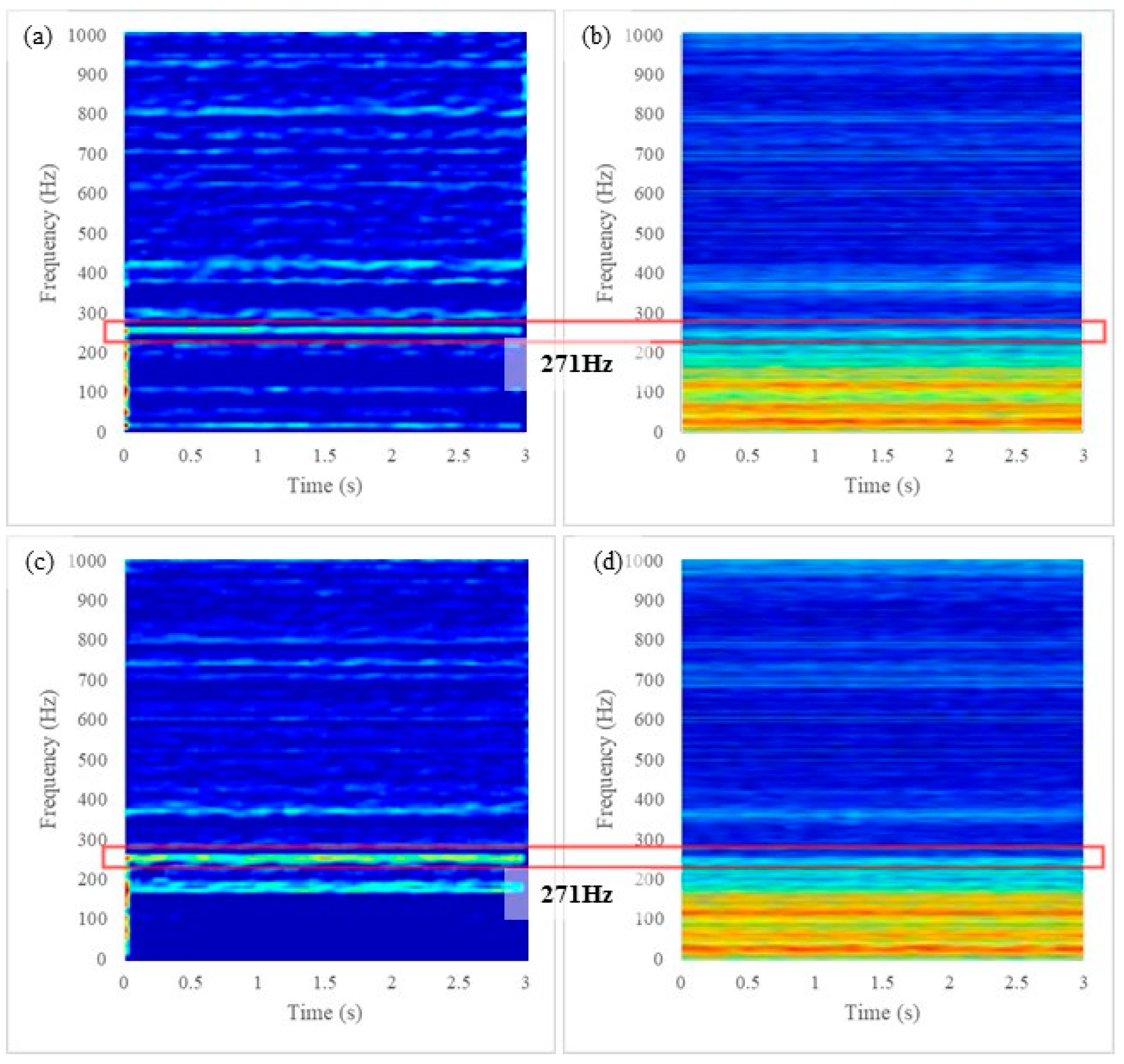
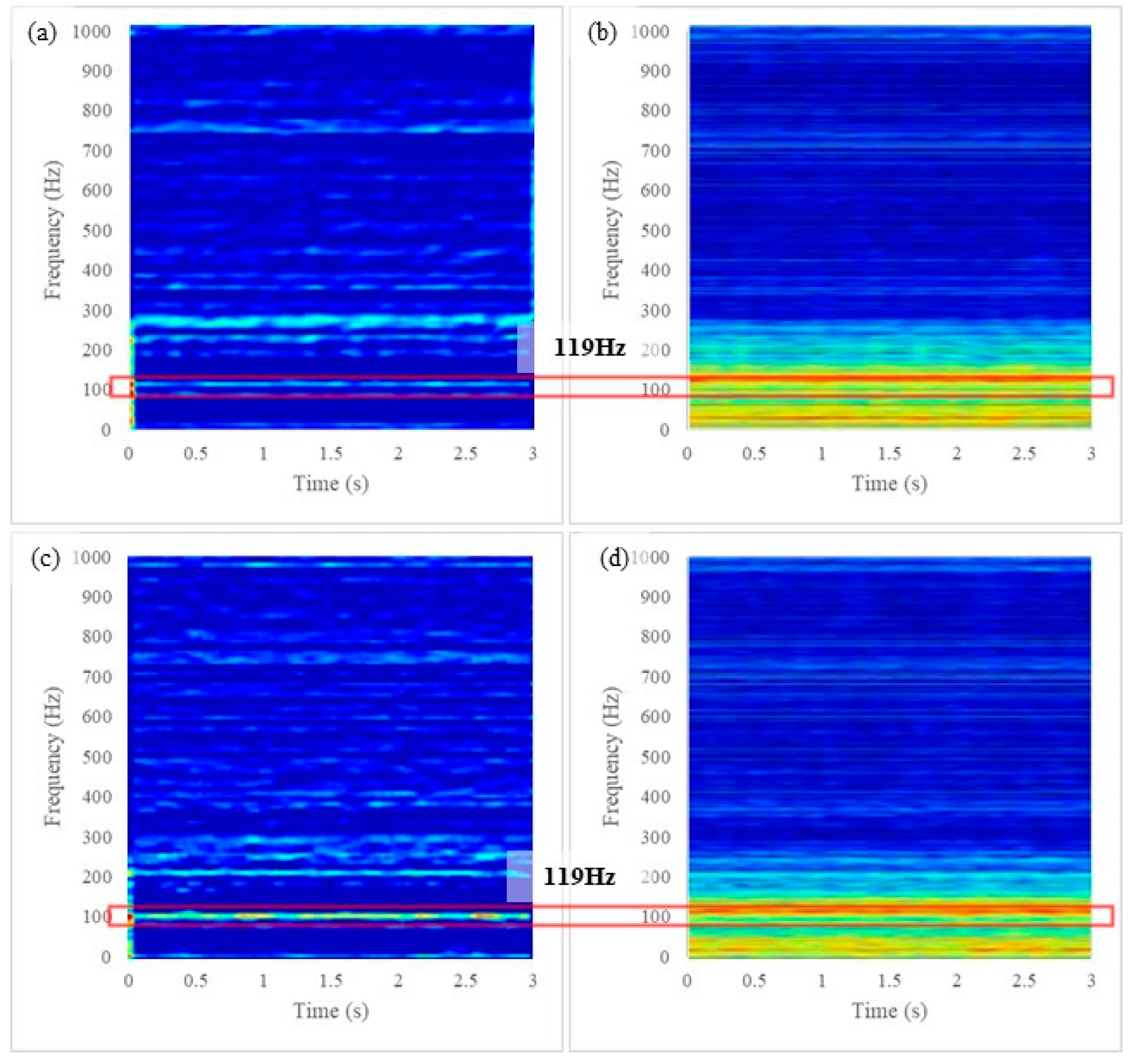
The model used for xAI analysis was NasNet, which has the highest classification accuracy. Spectrograms obtained from bearings in both inner race failure and outer race failure states were inputted into the trained NasNet, highlighting the regions considered in determining faults. As shown in Figure 13, Figure 14 and Figure 15, the frequency regions with high scores for fault detection are clearly marked with high scores on the scoremap. These common high-scoring feature points were compared to the theoretical fault frequencies of the bearings. The theoretical fault frequencies are related to the inner race (f_i) and outer race (f_o) failures calculated in Equations (1) and (2) below:

$$f_i={\displaystyle \frac{N}{2}}{f}_s\left(1+{\displaystyle \frac{D_b}{D_c}}cos\alpha \right)$$

(1)

$$f_o={\displaystyle \frac{N}{2}}{f}_s\left(1-{\displaystyle \frac{D_b}{D_c}}cos\alpha \right)$$

(2)

where N represents the static load, f_s is the rotation frequency, D_b is the ball bearing diameter, D_c is the pitch diameter, and α is the contact angle [30].

In Figure 13, the primary indicator of inner race failure is detected around 181 Hz, which matches the theoretical fault frequency calculated from the equations. Similarly, Figure 14 shows that at a rotation speed of 3000 RPM, the main fault frequency occurs at 271 Hz. Figure 15 verifies that the prominent feature in the scoremap corresponds with the theoretical fault frequency of 119 Hz for outer race failure. The features commonly identified in fault scenarios beyond the theoretical fault frequencies are empirical and derived through machine learning. This suggests the potential to develop a theoretical framework that can explain these empirically obtained features based on experimental results.

4. Conclusions

This study was initiated by identifying the high costs associated with the data collection devices currently used in bearing fault diagnosis systems. To address this issue, a low-cost sensor module utilizing affordable sensors was designed and proposed. The research demonstrated that this economical sensor module can effectively replace more expensive sensors and data acquisition devices, offering significant cost savings compared to traditional high-priced equipment. Additionally, the module boasts versatility and ease of installation, allowing for straightforward attachment and removal, which enhances its practicality for various applications.

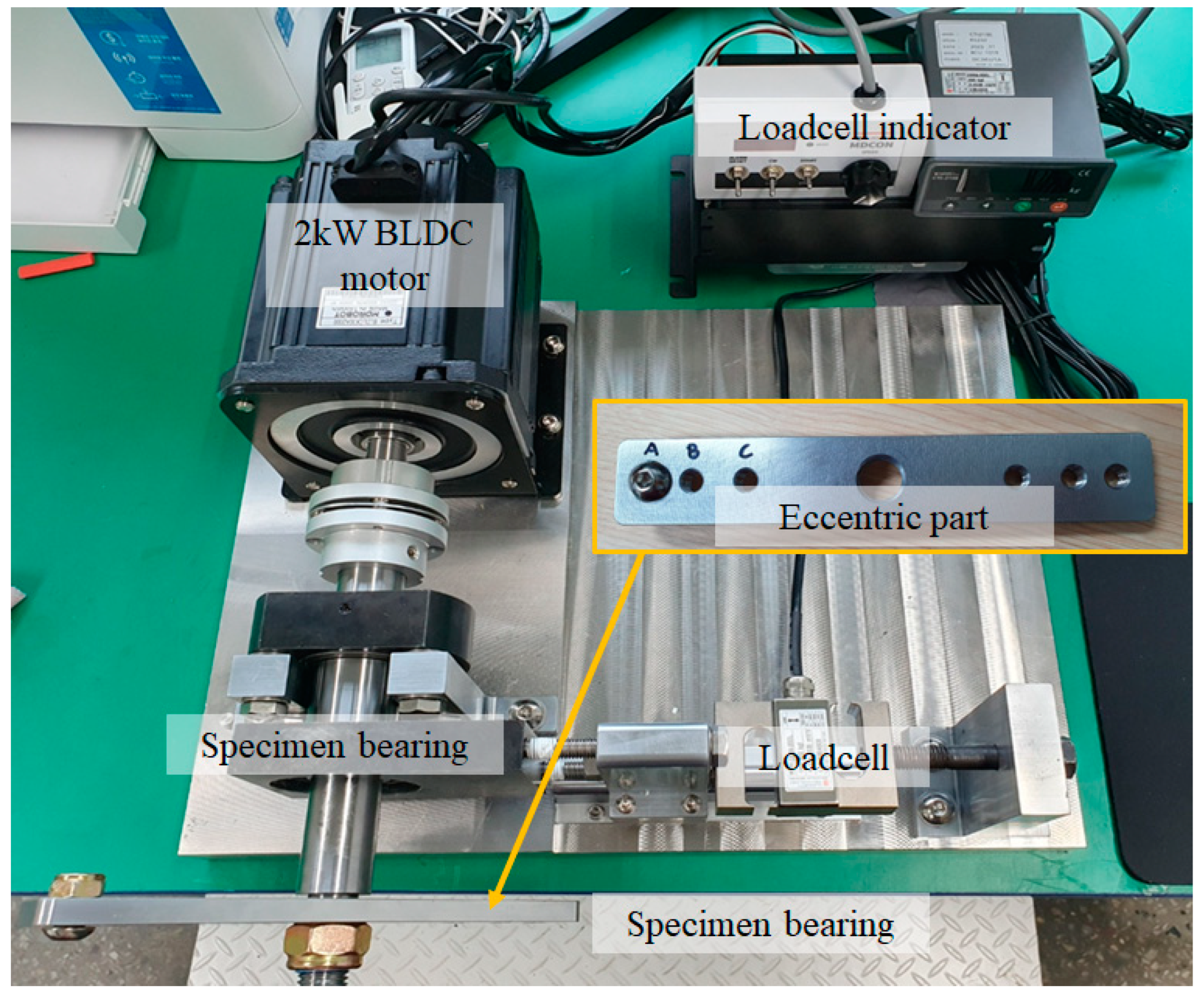
A test bed was assembled to emulate signals from both normal and faulty bearings. The setup included a motor, motor coupling, support bearings, specimen bearings, a rotating shaft, and a load cell, all constructed. Powered by a 2 kW BLDC motor capable of reaching up to 3000 RPM, the test bed effectively minimizes vibrations during high-speed rotation. Deep groove ball bearings were chosen as specimen bearings, while thrust needle bearings served as support bearings due to their higher safety factor for radial loads.

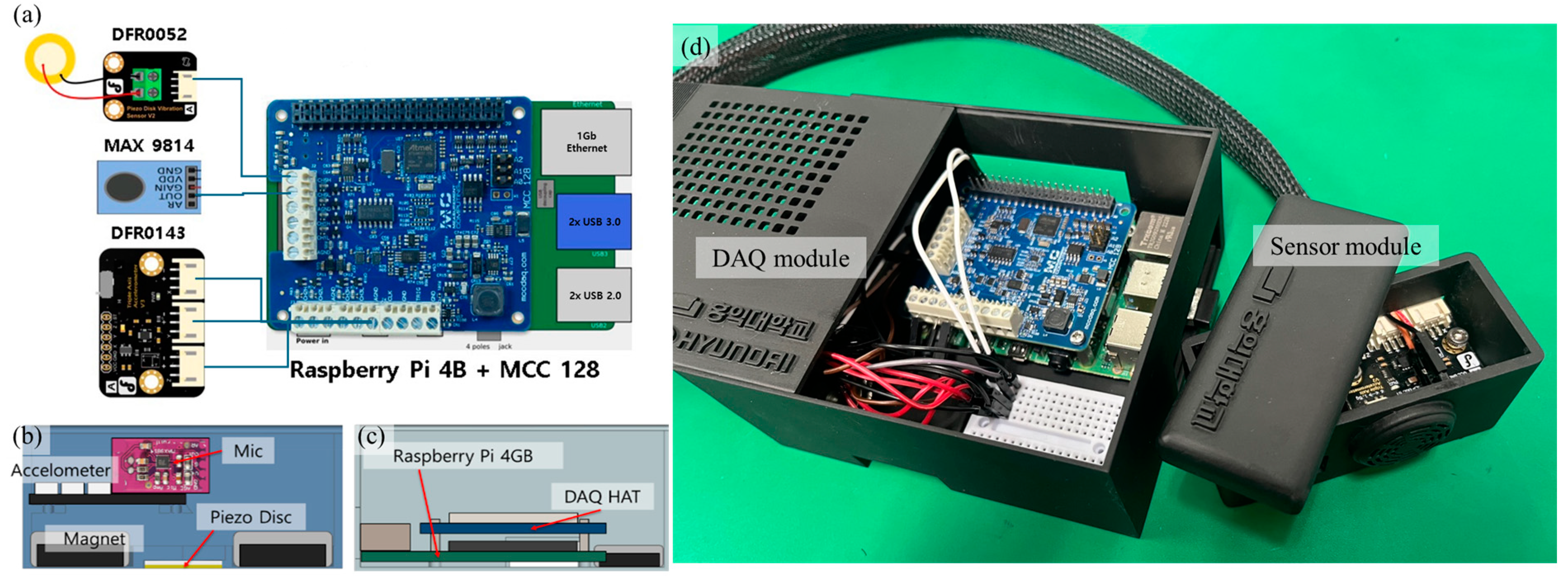
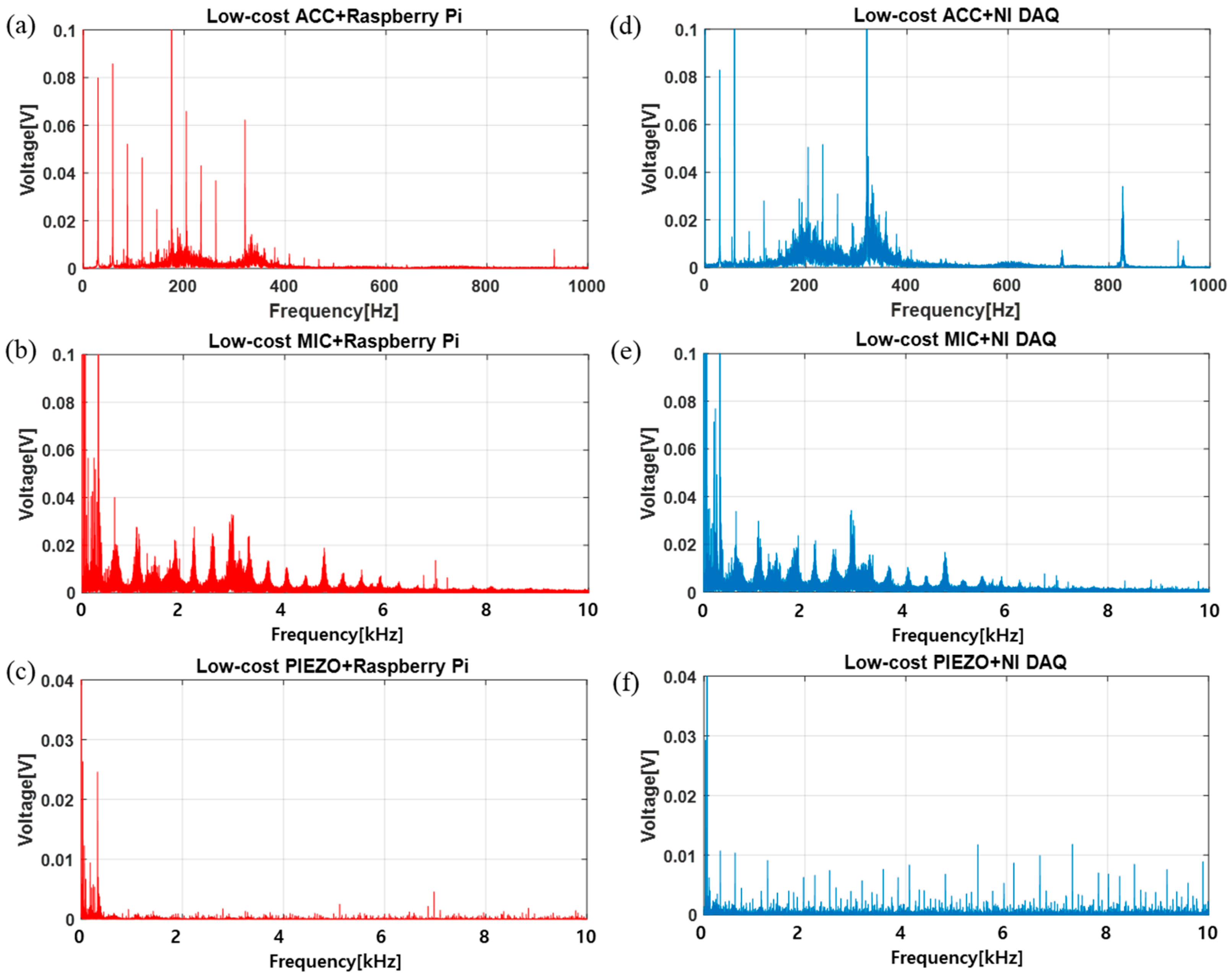
The low-cost monitoring system comprises a sensor module, which includes an accelerometer, microphone, and piezo disc, and a data acquisition module. A comparative study validated the reliability of the low-cost sensor against high-cost alternatives, revealing that the low-cost system costs approximately 3% of the price of expensive counterparts. Experimental results showed that the low-cost accelerometer performed similarly to high-cost versions at frequencies below 1 kHz, although some discrepancies were noted at higher frequencies. Additionally, the low-cost DAQ module demonstrated signal measurement performance comparable to that of high-cost systems, underscoring its potential as a viable replacement in industrial settings.

Data collection experiments were conducted under 72 different conditions, each repeated 10 times, resulting in 720 samples and 2160 time-series data points from three sensors. After preprocessing, the data were visualized as spectrograms and scalograms. The spectrograms utilized the Fourier transform to analyze frequency components over time, while the scalograms employed the wavelet transform for higher-resolution analysis of non-stationary signals. The visualized data, totaling 4320 images, were used to train DNN models. The study employed GoogLeNet, ResNet-50, and NasNet to classify bearings as either normal or faulty, with each model exhibiting distinct strengths. To enhance model reliability, an xAI technique was implemented to visualize the scores associated with each image, clarifying how the models made their decisions.

The research demonstrated that utilizing a low-cost monitoring system in conjunction with deep neural networks can effectively detect bearing failures, suggesting the potential for widespread implementation across various industrial sectors. Additionally, the study proposed a methodology using xAI techniques to understand the reasoning behind the DNN models’ fault assessments, indicating the potential for deriving new failure theories from the common characteristics identified by the models.

The proposed method aims to diagnose bearing faults using DNN based on data collected from low-cost sensors. However, the developed low-cost sensors have not undergone long-term reliability validation compared to high-cost sensors, necessitating a process for verifying their reliability over extended periods. Additionally, by miniaturizing the sensors and attaching them to flexible materials, enabling their application to machine surfaces of various shapes beyond traditional mounting methods, the effectiveness of the proposed approach is expected to be significantly enhanced in future work.

To verify the reliability of the proposed sensors and failure diagnosis methods, it is necessary to install them in a machine system that includes actual bearings and study whether they can detect signals generated when a bearing fails and analyze the failure in future work. Additionally, the research can be expanded to develop a model that predicts bearing life by detecting changes in signals as the bearing’s lifespan decreases.

References

1. Jiang, X.; Song, Q.; Wang, H.; Du, G.; Guo, J.; Shen, C.; Zhu, Z. Central frequency mode decomposition and its applications to the fault diagnosis of rotating machines. Mech. Mach. Theory 2022, 174, 104919. [Google Scholar] [CrossRef]
2. Wan, L.; Li, Y.; Chen, K.; Gong, K.; Li, C. A novel deep convolution multi-adversarial domain adaptation model for rolling bearing fault diagnosis. Measurement 2022, 191, 110752. [Google Scholar] [CrossRef]
3. Yang, Z.; Merrild, U.C.; Runge, M.T.; Pedersen, G.; Børsting, H. A study of rolling-element bearing fault diagnosis using motor’s vibration and current signatures. IFAC Proc. Vol. 2009, 42, 354–359. [Google Scholar] [CrossRef]
4. Zhou, L.; Duan, F.; Mba, D.; Wang, W.; Ojolo, S. Using frequency domain analysis techniques for diagnosis of planetary bearing defect in a CH-46E helicopter aft gearbox. Eng. Fail. Anal. 2018, 92, 71–83. [Google Scholar] [CrossRef]
5. SKF. Rolling Bearings. Available online: https://www.skf.com/binaries/pub12/Images/0901d196802809de-Rolling-bearings---17000_1-EN_tcm_12-121486.pdf (accessed on 13 November 2024).
6. NSK. Rolling Bearings. Available online: https://www.nsk.com/content/dam/nsk/common/catalogs/ctrgPdf/e1102m.pdf (accessed on 13 November 2024).
7. The Schaeffler Group. Large Size Bearings. Available online: https://www.schaeffler.com/remotemedien/media/_shared_media/08_media_library/01_publications/schaeffler_2/catalogue_1/downloads_6/gl1_de_en.pdf (accessed on 13 November 2024).
8. Zarei, J.; Poshtan, J. Bearing fault detection using wavelet packet transform of induction motor stator current. Tribol. Int. 2007, 40, 763–769. [Google Scholar] [CrossRef]
9. Zhang, P.; Du, Y.; Habetler, T.G.; Lu, B. A Survey of Condition Monitoring and Protection Methods for Medium-Voltage Induction Motors. IEEE Trans. Ind. Appl. 2010, 47, 34–46. [Google Scholar] [CrossRef]
10. Gangsar, P.; Tiwari, R. Signal based condition monitoring techniques for fault detection and diagnosis of induction motors: A state-of-the-art review. Mech. Syst. Signal Process. 2020, 144, 106908. [Google Scholar] [CrossRef]
11. SFK. SKF Proactive Reliability Maintenance. Available online: https://vehicleaftermarket.skf.com/binaries/pub12/Images/0901d196808adda2-18382-EN_SKF-Proactive-reliability-maintenance_tcm_12-482786.pdf (accessed on 13 November 2024).
12. Tahmasbi, D.; Shirali, H.; Souq, S.S.M.N.; Eslampanah, M. Diagnosis and root cause analysis of bearing failure using vibration analysis techniques. Eng. Fail. Anal. 2024, 158, 107954. [Google Scholar] [CrossRef]
13. Jakobsen, M.O.; Herskind, E.S.; Pedersen, C.F.; Knudsen, M.B. Detecting insufficient lubrication in rolling bearings, using a low cost MEMS microphone to measure vibrations. Mech. Syst. Signal Process. 2023, 200, 110553. [Google Scholar] [CrossRef]
14. Fang, Q.; Qiao, B.; Yu, M. A study on the feature separation and extraction of compound faults of bearings based on casing vibration signals. J. Vibroeng. 2021, 23, 1737–1752. [Google Scholar] [CrossRef]
15. Xu, Y.; Jiang, Q.; Li, S.; Zhao, Z.; Sun, B.; Huang, G.Q. Digital twin-driven discriminative graph learning networks for cross-domain bearing fault recognition. Comput. Ind. Eng. 2024, 193, 110292. [Google Scholar] [CrossRef]
16. Gunerkar, R.; Jalan, A. Classification of Ball Bearing Faults Using Vibro-Acoustic Sensor Data Fusion. Exp. Tech. 2019, 43, 635–643. [Google Scholar] [CrossRef]
17. Wang, L.; Robert, W.; Jun, S. Acoustic emissions from oil lubricated metal on metal sliding contacts. Insight-Non-Destr. Test. Cond. Monit. 2008, 50, 506–511. [Google Scholar] [CrossRef]
18. Chen, S.; Craig, M.; Wood, R.J.; Wang, L.; Callan, R.; Powrie, H. Bearing Condition Monitoring Using Multiple Sensors and Integrated Data Fusion Techniques. In Proceedings of the Ninth International Conference in Vibrations in Rotating Machinery, Exeter, UK, 8–10 September 2008; pp. 1–12. [Google Scholar]
19. Yang, Y.; Liu, H.; Ma, H.; Wang, P.; Han, Q.; Wen, B. Experimental study on vibration characteristics due to cage damage of deep groove ball bearing. Tribol. Int. 2023, 185, 108555. [Google Scholar] [CrossRef]
20. Doğan, B.K.; Karaçay, T. Experimental fault analysis of polymer hybrid bearing using accelerometer and load cell. Tribol. Int. 2023, 185, 108498. [Google Scholar] [CrossRef]
21. Zhang, P.; Pan, A.; Yan, K.; Zhu, Y.; Hong, J.; Liang, P. High-efficient and reversible temperature sensor fabricated from highly luminescent CdTe/ZnS-SiO2 nanocomposites for rolling bearings. Sens. Actuators A Phys. 2021, 328, 112758. [Google Scholar] [CrossRef]
22. Magadán, L.; Granda, J.; Suárez, F. Robust prediction of remaining useful lifetime of bearings using deep learning. Eng. Appl. Artif. Intell. 2024, 130, 107690. [Google Scholar] [CrossRef]
23. Ma, S.; Chu, F. Ensemble deep learning-based fault diagnosis of rotor bearing systems. Comput. Ind. 2019, 105, 143–152. [Google Scholar] [CrossRef]
24. Elforjani, M.; Shanbr, S. Prognosis of Bearing Acoustic Emission Signals Using Supervised Machine Learning. IEEE Trans. Ind. Electron. 2017, 65, 5864–5871. [Google Scholar] [CrossRef]
25. Hao, S.; Ge, F.-X.; Li, Y.; Jiang, J. Multisensor bearing fault diagnosis based on one-dimensional convolutional long short-term memory networks. Measurement 2020, 159, 107802. [Google Scholar] [CrossRef]
26. Zhang, W.; Li, C.; Peng, G.; Chen, Y.; Zhang, Z. A deep convolutional neural network with new training methods for bearing fault diagnosis under noisy environment and different working load. Mech. Syst. Signal Process. 2018, 100, 439–453. [Google Scholar] [CrossRef]
27. Yu, X.; Dong, F.; Ding, E.; Wu, S.; Fan, C. Rolling Bearing Fault Diagnosis Using Modified LFDA and EMD With Sensitive Feature Selection. IEEE Access 2017, 6, 3715–3730. [Google Scholar] [CrossRef]
28. Jia, F.; Lei, Y.; Lin, J.; Zhou, X.; Lu, N. Deep neural networks: A promising tool for fault characteristic mining and intelligent diagnosis of rotating machinery with massive data. Mech. Syst. Signal Process. 2016, 72, 303–315. [Google Scholar] [CrossRef]
29. Guo, X.; Chen, L.; Shen, C. Hierarchical adaptive deep convolution neural network and its application to bearing fault diagnosis. Measurement 2016, 93, 490–502. [Google Scholar] [CrossRef]
30. Gougam, F.; Rahmoune, C.; Benazzouz, D.; Merainani, B. Bearing fault diagnosis based on feature extraction of empirical wavelet transform (EWT) and fuzzy logic system (FLS) under variable operating conditions. J. Vibroeng. 2019, 21, 1636–1650. [Google Scholar] [CrossRef]
Figure 1. Image of the test bed for the experiment.
Machines 12 00843 g001
Figure 2. Schematics of (a) the sensors and monitoring system, (b) the sensor module, and (c) the DAQ module; (d) image of the monitoring system.
Machines 12 00843 g002
Figure 3. FFT graphs of signals from the low-cost sensor: (a) accelerometer, (b) microphone, and (c) piezo-based sensor and from the high-cost sensor: (d) accelerometer, (e) microphone, and (f) piezo-based sensor.
Machines 12 00843 g003
Figure 4. FFT graphs of signals from the low-cost DAQ module with the low-cost sensors: (a) accelerometer, (b) microphone, and (c) piezo-based sensor and from the low-cost DAQ module with the low-cost sensors: (d) accelerometer, (e) microphone, and (f) piezo-based sensor.
Machines 12 00843 g004
Figure 5. Images of (a) inner race failure and (b) outer race failure of the bearing.
Machines 12 00843 g005
Figure 6. Images of (a) testbed and low-cost monitoring system for the experiment and (b) total system for diagnosis of the bearing condition.
Machines 12 00843 g006
Figure 7. Flow chart for diagnosis of the bearing condition in real time.
Machines 12 00843 g007
Figure 8. Real time monitoring system.
Machines 12 00843 g008
Figure 9. Spectrograms of (a) normal bearing, (b) inner race failure, and (c) outer race failure; scalograms of (d) normal bearing, (e) inner race failure, and (f) outer race failure from the accelerometer at 2000 RPM in rotation speed, 50 kgf in static load, and no dynamic load.
Machines 12 00843 g009
Figure 10. Spectrograms of (a) normal bearing, (b) inner race failure, and (c) outer race failure; scalograms of (d) normal bearing, (e) inner race failure, and (f) outer race failure from the microphone at 2000 RPM in rotation speed, 50 kgf in static load, and no dynamic load.
Machines 12 00843 g010
Figure 11. Spectrograms of (a) normal bearing, (b) inner race failure, and (c) outer race failure; scalograms of (d) normal bearing, (e) inner race failure, and (f) outer race failure from the piezo sensor at 2000 RPM in rotation speed, 50 kgf in static load, and no dynamic load.
Machines 12 00843 g011
Figure 12. Convolution matrices of the diagnosis results from (a) GoogLeNet, (b) ResNet-50, and (c) NasNet.
Machines 12 00843 g012
Figure 13. (a) Scoremap and (b) original spectrogram for the first tested bearing, and (c) scoremap and (d) original spectrogram for the second tested bearing, both operating at a rotation speed of 2000 RPM and subjected to a static load of 200 kgf with inner race failure.
Machines 12 00843 g013
Figure 14. (a) Scoremap and (b) original spectrogram for the first tested bearing, and (c) scoremap and (d) original spectrogram for the second tested bearing, both operating at a rotation speed of 3000 RPM and subjected to a static load of 200 kgf with inner race failure.
Machines 12 00843 g014
Figure 15. (a) Scoremap and (b) original spectrogram for the first tested bearing, and (c) scoremap and (d) original spectrogram for the second tested bearing, both operating at a rotation speed of 2000 RPM and subjected to a static load of 100 kgf with outer race failure.
Machines 12 00843 g015