Abstract
Coordinate measuring machines are widely used in the industrial field due to their ease of automation. However, estimating the measurement uncertainty is a delicate task, especially when controlling for deviation, given the large number of factors that influence the measurement. A precise estimate of the uncertainty is crucial to avoid incorrect conformity assessments. The purpose of this study is to control geometrical-form tolerance specifications, taking into consideration their associated uncertainty. A surface fitting model based on the least squares criterion is proposed, allowing one to obtain the variance–covariance matrix by iterative calculation according to the Levenberg–Marquard optimization method. The form deviation is then evaluated following the Geometrical Product Specifications (GPS) Standard, and its associated uncertainty is estimated using the guide to the expression of uncertainty in measurement (GUM) propagation of the uncertainty law. Finally, the conformity assessment is performed based on the measured deviation and its associated uncertainty. Different results for the measurement of straightness, flatness, circularity, roundness, and cylindricity are presented and detailed. This model is thereafter validated by a Monte Carlo simulation, and interlaboratory comparisons of the obtained results were performed, which showed satisfactory outcome. This contribution is of great use to manufacturing companies and metrology laboratories, allowing them to meet the normative guidelines, which stipulates that each measurement result must be accompanied by its associated uncertainty.
1. Introduction
The precision and accuracy of coordinate measuring machines (CMMs) are crucial for quality control in manufacturing processes, as they ensure that components meet stringent design specifications. Understanding and quantifying form deviation uncertainty are essential for ensuring correct conformity assessments following the normative guidelines [1], which stipulate that each measurement result must be accompanied by its associated uncertainty.
Form deviation refers to the difference between a measured surface and its nominal geometry, as stated in the Geometric Product Specifications norm [2,3,4]. Numerous studies have explored methods to assess and estimate form deviation in CMM measurements. For instance, Forbes [5,6] described semi-analytical approaches based on rectangular distributions and Gaussian process models, which take into consideration the likely spatial correlation of form deviations. Shichang Du et al. [7] presented a method based on multivariate spatial statistics for estimating the form deviation considering the influence of machining conditions and spatial correlation.
In a related study, Habibi et al. [8,9] examined parallelism and perpendicularity assessment and uncertainty estimation based on the propagation of uncertainties [10,11]. However, the estimation of the surface parameters’ variances was based on repeatability. Jalid et al. [12,13,14] used the same method, based on orthogonal distance regression, to estimate the fitting parameters uncertainties.
Recent advancements in measurement technology have also led to the development of sophisticated algorithms for form deviation analysis. Jakubiec et al. [15,16] introduced a software fully compliant with the GPS [2,3,4] philosophy for the evaluation of dimensional and geometrical specification tolerances, which demonstrated significant improvements compared to conventional CMM methods. Furthermore, Cui et al. [17] focused on the comparison between the results obtained using the least squares method and the genetic optimization algorithm, applied to flatness and roundness, which showed almost identical results.
Despite major advances and the various methods in the form deviation uncertainty estimation [18,19,20], there remains a need for more comprehensive studies that integrate form deviation uncertainty analysis with practical conformity assessment procedures [21]. This research aims to bridge this gap by proposing a model, as shown in Figure 1, for estimating the uncertainty using the GUM [10] law or propagation, where surface fitting [22,23] and CMM probing uncertainty [24,25,26,27] are two key components to estimate the form deviation’s measurement uncertainty.

Figure 1.
Proposed model.
Accordingly, the conformity assessment is performed based on the measured deviation and its associated uncertainty according to the ISO 98-4 [28]. Different results for the measurement of straightness, flatness, circularity, roundness, and cylindricity are presented and detailed. The surface fitting algorithm based on the least squares method is validated by comparison [29] with the National Institute of Standards and Technology [30] database. The form deviation calculation and its associated uncertainty estimation will thereafter be validated by a Monte Carlo simulation [11] and interlaboratory comparisons of the obtained assessment results will be conducted with Measurement Control Center [31] according to the ISO13528 [32].
2. Materials and Methods
The objective is to propose a model that enables the estimation of form deviation, its associated uncertainty, and the conformity assessment with the specified standards, as shown in Figure 2. We start by probing a cloud of points Pi (xi, yi, zi) using the coordinate measuring machine. Initially, we performed a surface fitting, which generates the parameters and its covariance matrix . This covariance matrix is incorporated into the estimation of the form deviation uncertainty. Following this, we calculate the form deviation and its associated uncertainty, accounting for the probing error of the coordinate measuring machine. Finally, we declare conformity, taking into consideration the calculated uncertainty.

Figure 2.
Form tolerance control model.
A specific measurement process must be followed in order to control a geometrical specification:
- Surface probing.
- Surface fitting.
- Form deviation evaluation.
- Estimation of the form deviation associated uncertainty.
- Declaration of conformity.
The details of each of these steps will be provided in the following paragraphs.
2.1. Machine Probing Uncertainty
Coordinate measuring machines are precise and accurate. However, various factors influence the measurement uncertainty (Figure 3), and it is very difficult to quantify the influence of each of these parameters independently of the others.

Figure 3.
CMM measurement uncertainty sources.
Several approaches have been used for the estimation of the uncertainty associated with probing [33]. We will assume that the errors along the axes are independent and linear, and the uncertainty matrix associated with each probed point is given as follows:
where , , , with , where a and b are constants, and k the coverage factor defined by the law of the selected distribution. The variables a and b are determined by measuring 5 gauge blocks, each block for 3 repetitions, along 3 of the 7 directions specified in ISO 10360-2 [34], then calculating the error equations along each direction = x + (error following the direction X for example), then estimating the associated uncertainty .
2.2. Surface Fitting Parameters and Associated Variance–Covariance Matrix
Surface fitting is a mathematical modeling technique that enables the transition from a cloud of points extracted from the actual surface to an associated theoretical element that best represents it. Basic geometric elements can be represented in terms of their parameters. Let P be a point on the surface in question (as shown in Figure 4); it satisfies the following equations in Table 1.

Figure 4.
Parametrization of the studied elements: line, plane, circle, sphere and cylinder.

Table 1.
Geometrical elements’ equations.
We will base our approach on the least squares criterion, which involves minimizing the sum of squared residuals , where represents the orthogonal distance between the measured points and the substitute feature, as shown in Figure 5.

Figure 5.
Orthogonal distance between the point and the fitting feature.
Consider a point cloud probed using a coordinate measuring machine, on elements that are nominally linear, planar, circular, cylindrical, and spherical. We propose the following objective functions to obtain the substitute features parameters:
- Line:
- Plane:
- Circle:
- Sphere:
- Cylinder:
The least squares method tends to be more sensitive to outliers because it squares the errors. Significant errors have a greater impact, leading to a good overall fit to the data, but it does not necessarily ensure the smallest maximum error across the entire data range. Our objective is to minimize for the different values of the parameters :
A weighting can be introduced into the model such as:
- is the measurement uncertainty of the probed point.
- for points located in a critical area.
- for outliers.
Our optimization problem translates to the following nonlinear regression equation:
Solving the equation requires minimizing expressed by the equation:
with .
The variance–covariance matrix associated with the estimated parameters is expressed as
as represents the Jacobian matrix of evaluated at the estimated parameters , and the residual variance estimated by the following equation:
where is the number of parameters and is the number of measured points.
The estimated parameter associated uncertainty is given by .
2.3. Form Deviation Evaluation
After surface fitting, it is possible to evaluate the form deviation based on the fitting parameters (Section 2.2) of the geometric shapes and the probed points . We propose the following models for each specification:
where and are the extreme points that are the furthest apart perpendicularly to the vector :
2.4. Estimation of Form Deviation Associated Uncertainty
The determination of the combined uncertainty is the most critical step in the process and involves propagating the uncertainties of the error sources through the mathematical equation of the measurand , with based on a first-order Taylor series expansion. We assume that is statistically zero, such that and , and that the partial derivatives at the central point are constant. The variance can then be deduced as leading to the final form of the GUM uncertainty propagation law:
where represents the variance–covariance matrix, and is the Jacobian expressed as:
We then obtain the expanded uncertainty , where is the coverage factor and is the standard uncertainty. For a 95.45% confidence interval, the coverage factor is equal to 2.
2.5. Conformity Assessment
To establish a conformity assessment procedure for dimensional and geometric specifications taking into account the measurement uncertainty, it will be necessary to calculate the risk zone, assuming that uncertainty follows a normal distribution:
According to ISO/IEC Guide 98-4 [30], if the acceptable risk limit is not specified by the client, the risk n must not exceed 2.3%, where, is the Gaussian coefficient using the standard normal distribution, expressed as .
By incorporating measurement uncertainty into the conformity assessment process, the decisions made become more aligned with real-world situations and imposed standards, thereby improving quality control.
3. Proposed Algorithm
After modeling the steps outlined in the previous section, a data processing program was developed in MATLAB R2024b. Figure 2 presents the algorithm that illustrates the process. This program involves reading the data file containing the coordinates of the measured points. It will also require the type of the controlled specification, and its tolerance limit. As output, we obtain the measured form deviation, its associated uncertainty, and the conformity statement.
Depending on the geometry being controlled, the algorithm can require up to 7 starting parameters that can approximate the solution to avoid local optima and converge more effectively. represent the coordinates of a point, a vector, and a radius.
To determine the starting parameters [35,36], we will assume that the studied geometries are complete; therefore, the starting point will be the centroid, such as , , , where represents the total number of probed points.
In order to determine the starting normal vector for the plane and circle, and the starting direction vector for the line and the cylinder, we are going to use singular value decomposition. For example, is the eigenvector associated with the largest eigenvalue of , where A is the matrix whose row is . Alternatively, is the singular vector corresponding to the largest singular value of A for the direction vector and the smallest singular value of A for the normal vector.
Regarding the starting radius, it will be based on the following mean value of the radius; for example, the sphere and circle starting radius is given by the following equation:
Based on the probed points and the objective function (error function, detailed in Section 2.2), once the initial vector is determined, we can proceed to surface fitting. A nonlinear regression process is then applied, allowing us to obtain both the fitting parameters and the associated covariance matrix as shown in Figure 6.

Figure 6.
The surface fitting model.
The optimization method followed is the Levenberg–Marquardt algorithm [37], assuming that the objective function is smooth and differentiable allowing gradient information to be used effectively, and that the starting vector is a reasonable initial guess avoiding local optima. The algorithm combines the stability of gradient descent with the efficiency of the Gauss–Newton approach, making it particularly useful for curve fitting. This hybrid approach provides both stability and speed, addressing the weaknesses of each individual technique.
The form deviation is subsequently calculated from the data sets and the fitting parameters , by determining the extreme points M and m as detailed in Section 2.3. Therefore, based on the form deviation equation , the GUM law of uncertainty propagation is applied, as shown in Figure 7, and the result is expressed in matrix form as .

Figure 7.
Form deviation uncertainty estimation model.
The calculation of the Jacobian is detailed in Annex B, and the matrix is constructed from the uncertainty associated with the extreme points M and m, resulting from the CMM probing error, as well as the uncertainty from the surface fitting, depending on the parameters influencing the form deviation.
It is important not to confuse the parameters with , as represents the number of parameters in the deviation equation and represents the number of fitting parameters related to the fitted feature.
Finally, the declaration of conformity will be made based on the calculated deviation and its associated uncertainty, in accordance with ISO standard 98-4 [28], by applying Equation (14), with a risk not exceeding 2.3% unless specified by the customer.
4. Results
In this paragraph, we will address examples of geometric form specifications on different mechanical parts, namely, 10 μm straightness, 10 μm flatness, 15 μm circularity, 15 μm sphericity, and 15 μm cylindricity deviation tolerance limits from features that are, respectively, nominally linear, plane, circular, spherical, and cylindrical. The probed point datasets for each experiment are provided in Table A1, Table A2 and Table A3.
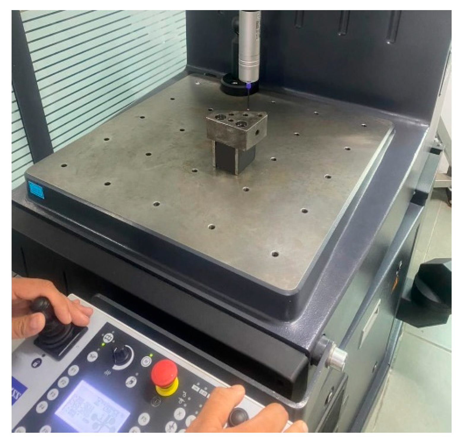
As shown in Figure 8, the CMM used is a Mitutoyo Euro-C 544 (Kanagawa, Japan), with a measuring volume of 500 × 400 × 400 mm3. It offers an MPE (Maximum Permissible Error) for length measurement of 2.9 + 4 L/1000 µm within the temperature range of 18 °C to 22 °C coupled with a TP2 type probe head mounted with a tungsten carbide stylus of effective working length EWL = 14 mm and a ruby tip of diameter D = 2 mm, all controlled by Mcosmos Geopack software. The temperature is regulated at 20° ± 2 °C and the probing speed is set to 10 mm/s.
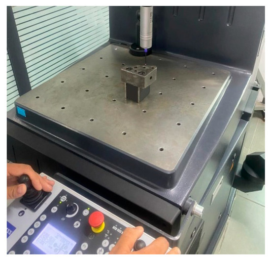
Figure 8.
The coordinate measuring machine used for probing the inspected parts.
We begin by probing the point dataset, accounting for the probing uncertainty associated with each measured point , where .
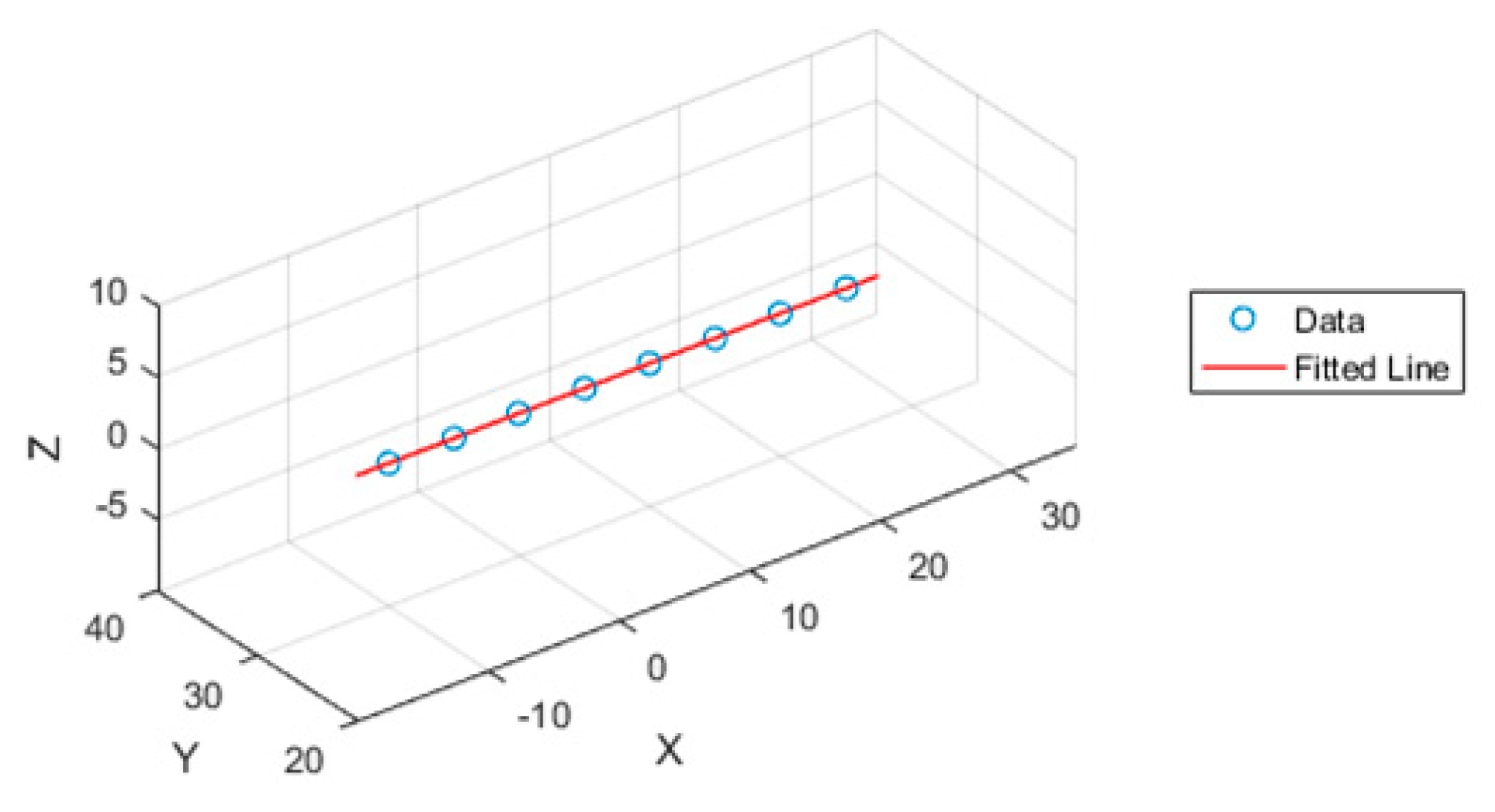
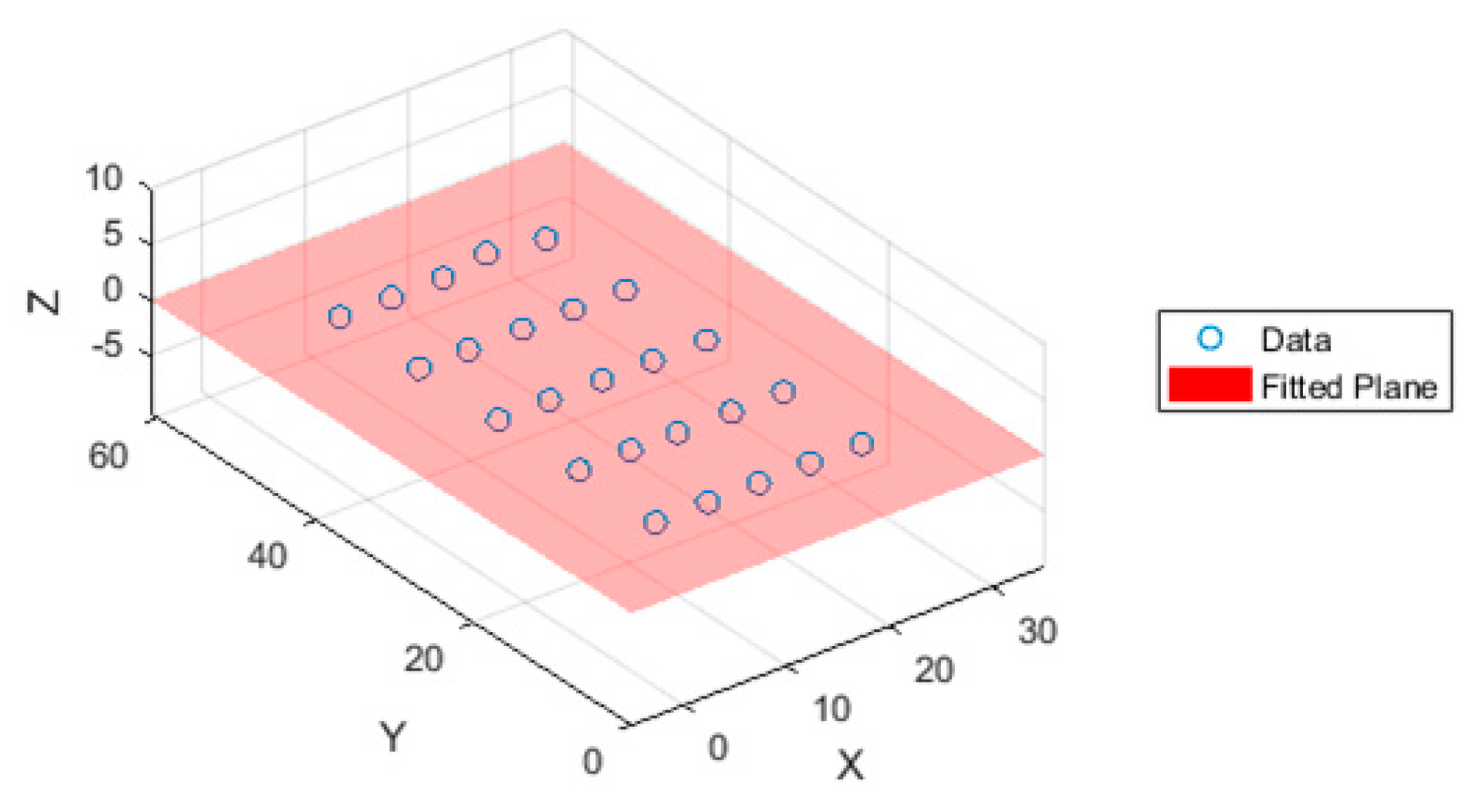
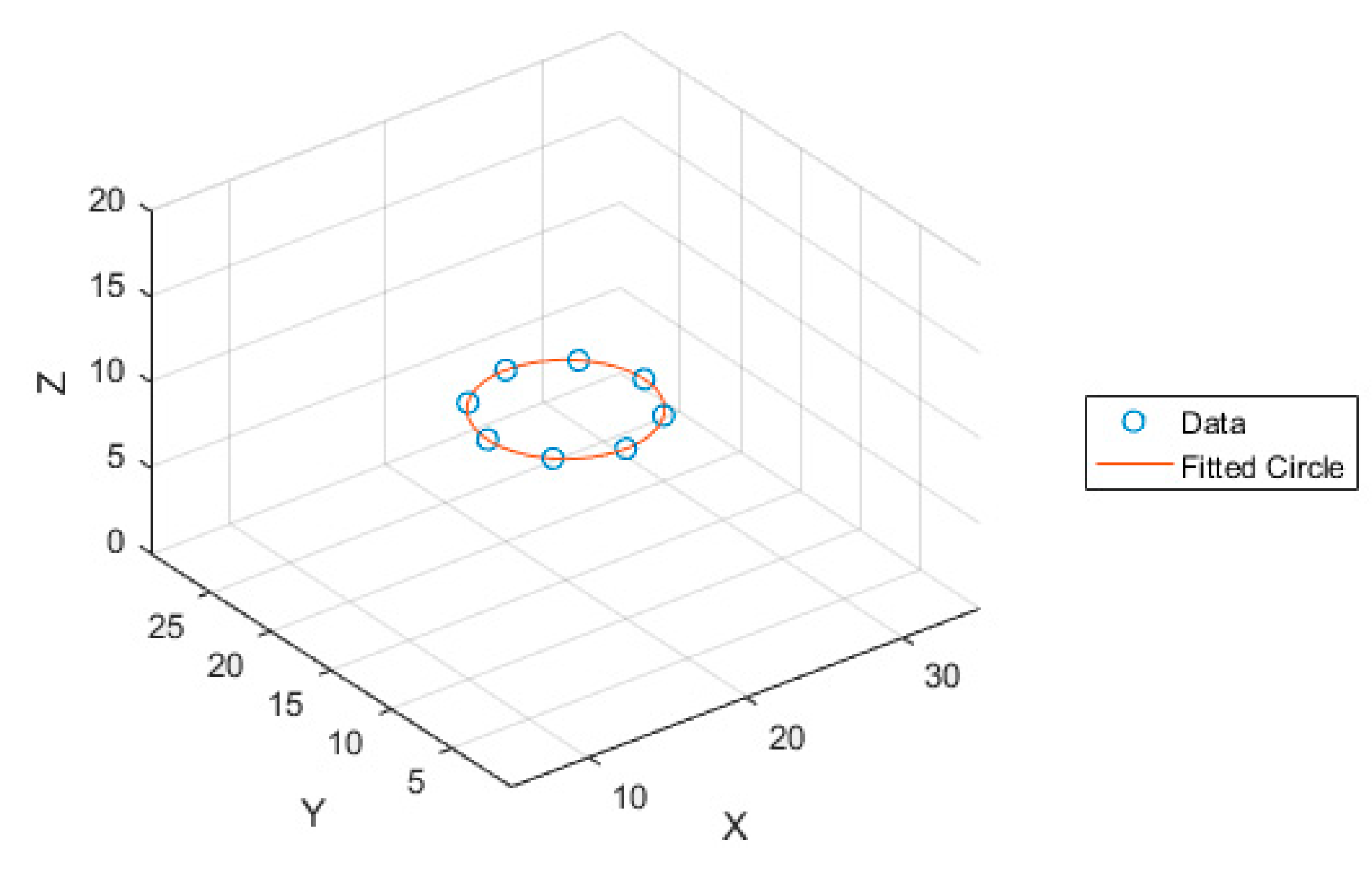
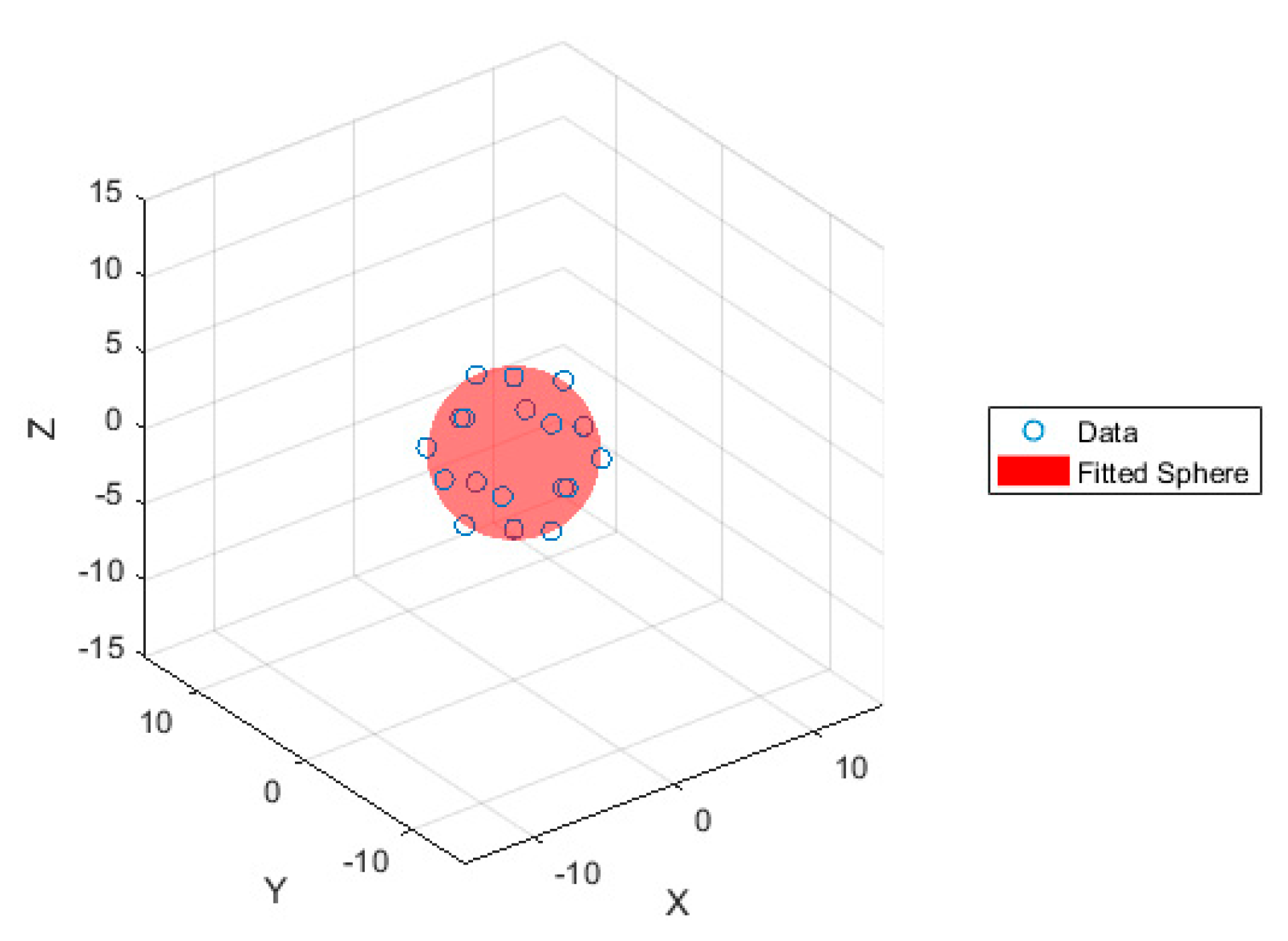
Subsequently, we perform surface fitting to obtain the fitting parameters β. The resulting fitting covariance matrix is then utilized for uncertainty estimation. Figure 9, Figure 10, Figure 11, Figure 12 and Figure 13 illustrate the probed points and the fitted features for the line, plane, circle, sphere, and cylinder. The form deviation is evaluated by identifying the two extreme points and . The Jacobian matrix is computed, and the variance–covariance matrix is constructed, allowing us to accurately estimate the form deviation and its associated uncertainty calculated as .
More detailed calculations of the different form deviations and the Jacobian are provided in Appendix B. In the following examples, we will briefly outline the key results relevant for each step to control the different specifications.
4.1. Straightness
- -
- Probing of the point dataset and surface fitting:
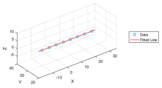
Figure 9.
Line fitting.
Figure 9.
Line fitting.
- -
- Determination of the two extreme points:
- -
- Calculation of the Jacobian, and construction of the variance–covariance matrix:
- -
- Estimation of straightness deviation and its associated uncertainty:
4.2. Flatness
- -
- Probing of the point dataset and surface fitting:

Figure 10.
Plane fitting.
Figure 10.
Plane fitting.
- -
- Determination of the two extreme points:
- -
- Calculation of the Jacobian and construction of the variance–covariance matrix:
- -
- Estimation of flatness deviation and its associated uncertainty:
4.3. Circularity
- -
- Probing of the point dataset and surface fitting:
Figure 11.
Circle fitting.
Figure 11.
Circle fitting.
- -
- Determination of the two extreme points:
- -
- Calculation of the Jacobian and construction of the variance–covariance matrix:
- -
- Estimation of circularity deviation and its associated uncertainty:
4.4. Sphericity
- -
- Probing of the point dataset and surface fitting:
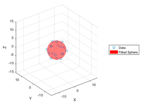
Figure 12.
Sphere fitting.
Figure 12.
Sphere fitting.
- -
- Determination of the two extreme points:
- -
- Calculation of the Jacobian and construction of the variance–covariance matrix:
- -
- Estimation of sphericity deviation and its associated uncertainty:
4.5. Cylindricity
- -
- Probing of the point dataset and surface fitting:
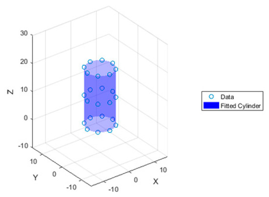
Figure 13.
Cylinder fitting.
Figure 13.
Cylinder fitting.

- -
- Determination of the two extreme points:
- -
- Calculation of the Jacobian and construction of the variance–covariance matrix:
- -
- Estimation of cylindricity deviation and its associated uncertainty:
5. Validation of the Proposed Model
In this section, we will initially validate our algorithm, proposed by the Mechanical and Thermal Processes and Controls (PCMT) laboratory for estimating the parameters of the fitted geometrical features, by comparing our results with those provided by National Institute of Standards and Technology (NIST). Subsequently, we will conduct Monte Carlo simulations to validate the measurement uncertainty estimation method, based on the results obtained in Section 4. We will then conclude with an inter-laboratory comparison with the Measurement Control Center (MCC) laboratory. This combined approach, as shown in Table 2, ensures a comprehensive and rigorous validation of uncertainty estimates, thereby ensuring the consistency of our model.

Table 2.
The validation methods employed.
5.1. Validation of the Surface Fitting Parameters Algorithm
NIST (National Institute of Standards and Technology) provides point datasets sampled from various surfaces along with their corresponding parameters. We used their results as references to validate our method, highlighting common optimization problems such as convergence, local optima, and computation time. We studied different cases for each geometry (Figure 14). The results in Table 3 below represent the cases with the largest deviations found for each geometry (sphere, plane, line, cylinder, circle) for a resolution of mm.
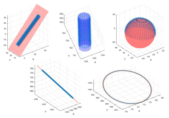
Figure 14.
NIST reference elements with the highest deviations.

Table 3.
Results of the surface fitting parameters comparison (all dimensions in mm).
We observe that the direction vector of the fitted cylinder is not equal to its reference vector (same norm, opposite direction). However, this will not impact the form deviation calculation and its associated uncertainty estimation.
Comparisons with the various reference geometrical elements yielded positive results. According to the classification proposed by NIST, our model falls under “Category 1”, characterized by its precision (deviations of less than 0.1 µm for linear distances, and less than 0.1 arc seconds for angular measurements), thus ensuring the reliability and accuracy of the results obtained. Compliance with NIST standards reinforces the credibility of our model, demonstrating that our approach aligns with best practices established by recognized experts in the field.
5.2. Validation of the Form-Deviation-Associated Uncertainty Estimation Method (Monte Carlo Simulation)
A Monte Carlo simulation is often used to validate the results of the uncertainty propagation method using the GUM method by determining if the confidence intervals obtained by the two methods are in agreement with a numerical tolerance. The validation procedure involved determining the confidence interval limits, and , using the GUM method (), where represents the expanded uncertainty obtained by the GUM method, and is the measured value of the form deviation. A Monte Carlo simulation is then conducted to obtain the confidence interval limits and , corresponding to the 95.45% confidence interval limits (), where is the mean and is the standard deviation from the obtained probability density. We then calculate and , the absolute differences between the respective limits of the GUM and Monte Carlo confidence intervals:
The validation was based on the comparison of these confidence interval limits. To ensure the adequacy of the significant digits provided by the GUM uncertainty, we calculated the numerical tolerance associated with the measurement process, , where is the number of significant digits after the decimal point. The validation criterion was that both and should be strictly less than :
If this condition is met, the comparison is favorable, confirming the validity of the GUM framework in this case.
We generated a distribution for a sample size of . The Box–Muller [38] algorithm was employed for the generation of the random values. For instance, in the case of the studied flatness deviation, we obtained the following distribution in Figure 15.
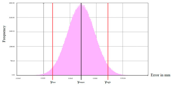
Figure 15.
Flatness deviation generated distribution.
From this generated distribution, we extracted the confidence interval limits and , as well as the mean , which allowed us to deduce the standard deviation . Similarly, for each of the other studied specifications, distributions were generated, enabling us to compare the results obtained by our GUM-based model with the Monte Carlo numerical method, as presented in Table 4.

Table 4.
Monte Carlo simulation results.
We note that in our case, the uncertainty estimated by the Monte Carlo simulation is greater than or equal to that of our proposed model, due to negative covariance components in our model, unlike the Monte Carlo numerical model based solely on variances (positive).
The machine’s numerical tolerance ζ = 0.5 × 10⁻³ mm is greater than all the calculated and values. The criterion is therefore satisfied, thus validating our uncertainty estimation model.
5.3. Inter-Laboratory Comparison
The inter-laboratory comparison was conducted with Measurement Control Center. The CMM used is a Zeiss Duramax (Oberkochen, Germany), with a measuring volume of 500 × 500 × 500 mm3. It complies with the ISO 10360-2:2009 standard [34], offering an MPE for length measurement (E0/E40) of 2.4 + L/300 µm within the temperature range of 18 °C to 22 °C coupled with a Vast-xxt-tl3 probe head mounted with a tungsten carbide stylus of effective working length EWL = 30 mm and a ruby tip of diameter D = 2 mm, all controlled by Calypso software. The temperature was regulated at 20° ± 2 °C and the probing speed was set at 10 mm/s. Although various evaluation techniques exist, the calculation of normalized error [32] is the most commonly employed method:
where and are the form deviations measured by the two laboratories, and and are, respectively, the uncertainties associated with these measurements. For the results to be considered valid, the normalized error must be less than 1. This ensures that the differences between the measurements from the two laboratories are within acceptable limits, accounting for the associated uncertainties.
The same industrial parts (Section 4) were measured under the same conditions and measurement range, we obtained the results summarized in Table 5.

Table 5.
Inter-laboratory comparison results.
It is noteworthy that the values measured by MCC fall within the uncertainty interval we estimated, thus supporting the consistency of our model.
The normalized deviations calculated between the results of PCMT and MCC laboratories are strictly less than 1. The criterion is therefore satisfied, validating our uncertainty estimation model, as well as the consistency of the results.
Despite the conclusive results of the normalized deviations, we notice contradictions in the conformity assessment. This is mainly due to an underestimation of measurement uncertainty by the MCC laboratory, which refers to the machine calibration to propose an uncertainty considering only the measurement ranges, as well as a difference in the conformity declaration criterion , where and are, respectively, the measured deviation and its associated uncertainty and the is the specified tolerance.
6. Conclusions
In conclusion, this study offers a framework for controlling geometrical form tolerance specifications by focusing on the accurate estimation of measurement uncertainty in coordinate measuring machines, thus aligning with ISO 17025 standards [1]. Based on the GUM law of propagation, it integrates surface fitting and CMM probing uncertainty as key components in estimating the measurement uncertainty of form deviations. Thereafter, the conformity assessment following ISO 98-4 is conducted considering the estimated uncertainty.
Coordinate measuring machines generally exhibit strong performance when measuring large to medium-sized dimensional features. However, when it comes to relatively small geometrical features, we observe a high repeatability relative to the size of the measured deviation, which aligns with the results obtained. Consequently, we focused on parts with minor form deviations, ranging from a mm flatness to a mm sphericity deviation; the estimated uncertainty reached nearly of the measured deviation value , mainly due to the machine’s capability. To reduce this uncertainty, several actions can be taken:
- -
- Increasing the number of probed points , leading to a decrease in the residual variance , which has a direct impact on the covariance matrix , ultimately resulting in lower measurement uncertainty.
- -
- Ensuring better distribution of probed points on the controlled surface, which enhances the accuracy of the surface representation, reducing the likelihood of biases and gaps in the data that could lead to poor initial estimates for the fitting parameters.
- -
- Applying a low weighting factor (k < 1) to outliers. Significant errors can disproportionately affect the results when using the least squares method, as it tends to be particularly sensitive to outliers because it squares the errors, magnifying their impact on the overall fitting process.
- -
- Calibrating the machine, reducing probing speed, maintaining the temperature regulated at 20° ± 2 °C, choosing a stylus with short effective working length, etc., thus allowing for the minimization of the uncertainty associated with probing and consequently lowering the measurement uncertainty.
The validation of this model through Monte Carlo numerical simulations confirmed its accuracy and reliability, as the maximum error between the confidence intervals compared to the GUM analytic method did not exceed mm, which remained significantly lower than the machine’s numerical tolerance ζ = 0.5 × 10⁻³ mm. The interlaboratory comparison conducted in accordance with ISO 13528 [32] yielded satisfactory results, as the largest normalized error was within the standards, further substantiating the model’s effectiveness. These findings underscore the model’s potential to enhance measurement practices in industrial settings, particularly in manufacturing companies and metrology laboratories, improving measurement accuracy and conformity assessments in various applications.
Author Contributions
Conceptualization, N.H., A.J. and A.S.; methodology, N.H., A.J. and A.S.; software, N.H.; validation, A.J. and A.S.; formal analysis, N.H.; investigation, N.H.; resources, N.H.; data curation, N.H. and A.S.; writing—original draft preparation, N.H.; writing—review and editing, A.J. and A.S.; supervision, A.J. and A.S.; project administration, A.J. and A.S.; All authors have read and agreed to the published version of the manuscript.
Funding
This research received no external funding.
Data Availability Statement
The original contributions presented in the study are included in the article, further inquiries can be directed to the corresponding authors.
Conflicts of Interest
The authors declare no conflicts of interest.
Appendix A
This appendix provides the coordinates of the points probed using the Coordinate Measuring Machine.

Table A1.
Coordinates of the points probed from the line and the circle.
Table A1.
Coordinates of the points probed from the line and the circle.
| Line | Circle | ||||
|---|---|---|---|---|---|
| x | y | z | x | y | z |
| −9.9856 | 30.0019 | 0.0061 | 24.9996 | 15.0007 | 10.0001 |
| −4.9842 | 30.0 | 0.0077 | 23.5398 | 18.5305 | 10.0002 |
| −0.0347 | 30.0031 | 0.0072 | 20.0006 | 19.9997 | 9.9999 |
| 5.0178 | 29.9974 | 0.0063 | 16.4797 | 18.5391 | 10.0001 |
| 9.9783 | 30.0016 | 0.0058 | 14.9994 | 15.0001 | 9.9998 |
| 14.9966 | 30.0 | 0.0072 | 16.4694 | 11.4602 | 9.9998 |
| 19.9726 | 30.0024 | 0.0047 | 20.0004 | 10.0001 | 9.9999 |
| 25.0317 | 29.9998 | 0.0036 | 23.5396 | 11.4699 | 9.9999 |

Table A2.
Coordinates of the points probed from the plane and the cylinder.
Table A2.
Coordinates of the points probed from the plane and the cylinder.
| Plane | Cylinder | ||||
|---|---|---|---|---|---|
| x | y | z | x | y | z |
| 4.9219 | 9.972 | 0.0026 | 4.9994 | 0.0002 | −0.0003 |
| 5.2049 | 20.0021 | 0.0047 | 3.5351 | 3.545 | 0.0003 |
| 5.0133 | 30.011 | 0.0044 | −0.0001 | 5.0005 | −0.0004 |
| 4.9998 | 40.018 | 0.0049 | −3.5348 | 3.5349 | 0.0006 |
| 4.9629 | 50.0275 | 0.0065 | −5.0003 | −0.0003 | −0.0002 |
| 10.0416 | 10.0348 | 0.005 | −3.5351 | −3.5352 | −0.0006 |
| 10.2183 | 20.0059 | 0.0069 | 0.0 | −5.0001 | −0.0 |
| 10.006 | 30.02 | 0.005 | 3.535 | −3.5347 | 0.0 |
| 9.7648 | 39.9959 | 0.0086 | 5.0 | 0.0001 | 10.0 |
| 9.9785 | 50.0021 | 0.0076 | 3.5348 | 3.5348 | 10.0002 |
| 15.0064 | 9.9988 | 0.0083 | 0.0001 | 5.0002 | 10.001 |
| 14.7649 | 20.0022 | 0.0099 | −3.535 | 3.5348 | 9.9999 |
| 15.111 | 30.0036 | 0.0085 | −4.9999 | −0.0002 | 10.0004 |
| 15.02 | 40.0082 | 0.0097 | −3.5349 | −3.5352 | 9.9997 |
| 14.9722 | 50.0027 | 0.0065 | −0.0001 | −4.9999 | 10.0001 |
| 19.9854 | 10.0043 | 0.0054 | 3.5351 | −3.5351 | 9.9996 |
| 19.9845 | 20.0014 | 0.0091 | 5.0001 | −0.0002 | 20.0008 |
| 20.0342 | 30.06 | 0.0066 | 3.5352 | 3.5349 | 20.0005 |
| 20.0171 | 40.0035 | 0.0074 | −0.0 | 5.0004 | 19.9997 |
| 19.9783 | 50.9976 | 0.0074 | −3.5348 | 3.5347 | 19.9991 |
| 24.9961 | 10.0013 | 0.0061 | −5.0001 | −0.0004 | 20.0 |
| 25.0317 | 20.06 | 0.0057 | −3.5351 | −3.5354 | 20.0002 |
| 25.2187 | 30.0026 | 0.0077 | −0.0001 | −4.9996 | 20.0001 |
| 25.0159 | 39.9991 | 0.0042 | 3.5349 | −3.5352 | 19.9999 |
| 24.9788 | 50.0051 | 0.0037 |

Table A3.
Coordinates of the points probed from the sphere.
Table A3.
Coordinates of the points probed from the sphere.
| Sphere | ||
|---|---|---|
| x | y | z |
| 5.0022 | −0.0091 | −0.0041 |
| 3.5407 | 3.5373 | −0.0041 |
| −0.0041 | 5.0025 | 0.0003 |
| −3.5352 | 3.5328 | −0.0002 |
| −5.005 | −0.0056 | 0.002 |
| −3.5363 | −3.5327 | 0.0097 |
| −0.0066 | −5.0023 | 0.0042 |
| 3.5361 | −3.5401 | 0.0028 |
| 0.0032 | 5.0029 | 0.0017 |
| 0.0007 | 3.5275 | 3.5362 |
| −0.0009 | 0.0077 | 4.9918 |
| −0.0003 | −3.5393 | 3.5294 |
| −0.0061 | −4.995 | −0.004 |
| −0.0012 | −3.5358 | −3.528 |
| −0.0031 | −0.0038 | −5.0032 |
| −0.0033 | 3.5244 | −3.5393 |
| 5.004 | 0.0101 | 0.0015 |
| 3.536 | −0.0097 | 3.5311 |
| −0.0008 | −0.0066 | 5.0035 |
| −3.5337 | 0.0055 | 3.5396 |
| −5.0068 | −0.0011 | 0.0043 |
Appendix B
This appendix includes detailed calculations of the different form deviations and the sensitivity components of the Jacobian.
- Straightness:
The form deviation is given by the following equation:
The sensitivity components are obtained as follows:
- Flatness:
The form deviation is given by the following equation:
The sensitivity components are obtained as follows:
- Circularity:
The form deviation will be given by the following equation:
The sensitivity components are obtained as follows:
- Cylindricity:
The form deviation is given by the following equation:
The same calculations as for the circularity apply, with the normal vector replaced by the direction vector .
- Sphericity:
The form deviation will be given by the following equation:
The sensitivity components are obtained as follows:
References
- ISO 17025:2017; General Requirements for the Competence of Testing and Calibration Laboratories. International Organization for Standardization: Geneva, Switzerland, 2017.
- ISO 1101:2017; Geometrical Product Specifications (GPS) Geometrical Tolerancing—Tolerances of Form, Orientation, Location and Run-Out. International Organization for Standardization: Geneva, Switzerland, 2017.
- ISO 10012:2003; Measurement Management Systems—Requirements for Measurement Processes and Measuring Equipment. International Organization for Standardization: Geneva, Switzerland, 2003.
- ISO 14253-2:2011; Geometrical Product Specifications (GPS)—Inspection by Measurement of Workpieces and Measuring Equipment—Part 2: Guide for the Estimation of Uncertainty in GPS Measurement, in Calibration of Measuring Equipment and in Product Verification. International Organization for Standardization: Geneva, Switzerland, 2011.
- Forbes, A. Uncertainty associated with form assessment in coordinate metrology. Int. J. Metrol. Qual. Eng. 2013, 4, 17–22. [Google Scholar] [CrossRef]
- Forbes, A. Measurement uncertainty and optimized conformance assessment. Measurement 2006, 39, 9. [Google Scholar] [CrossRef]
- Du, S.; Fei, L. Co-Kriging Method for Form Error Estimation Incorporating Condition Variable Measurements. J. Manuf. Sci. Eng. 2015, 138, 041003. [Google Scholar] [CrossRef]
- Habibi, N.; Jalid, A.; Salih, A.; Es-sadek, M.Z. Perpendicularity assessment and uncertainty estimation using coordinate measuring machine. Int. J. Metrol. Qual. Eng. 2023, 14, 12. [Google Scholar] [CrossRef]
- Habibi, N.; Jalid, A.; Salih, A.; Hanane, H. Estimation of parallelism measurement uncertainty according to the Geometrical Product Specifications standard using coordinate measuring machine. Int. J. Metrol. Qual. Eng. 2023, 14, 4. [Google Scholar] [CrossRef]
- JCGM 100:2008; Evaluation of Measurement Data—Guide to the Expression of Uncertainty in Measurement. International Organization for Standardization: Geneva, Switzerland, 2008.
- JCGM 101:2008; Evaluation of Measurement Data Supplement 1 to the Guide to the Expression of Uncertainty in Measurement—Propagation of Distributions Using a Monte Carlo Method. International Organization for Standardization: Geneva, Switzerland, 2008.
- Jalid, A.; Hariri, S.; Senelaer, J.P. Estimation of form deviation and the associated uncertainty in coordinate metrology. Int. J. Qual. Reliab. Manag. 2015, 32, 456–471. [Google Scholar] [CrossRef]
- Jalid, A.; Hariri, S.; El Gharad, A.; Senelaer, J.P. Comparison of the GUM and Monte Carlo methods on the flatness uncertainty estimation in coordinate measuring machine. Int. J. Metrol. Qual. Eng. 2016, 7, 302. [Google Scholar] [CrossRef]
- Jalid, A.; Hariri, S.; Laghzale, N.E. Influence of sample size on flatness estimation and uncertainty in three-dimensional measurement. Int. J. Metrol. Qual. Eng. 2015, 6, 102. [Google Scholar] [CrossRef]
- Jakubiec, W.; Płowucha, W. First Coordinate Measurements Uncertainty Evaluation Software Fully Consistent with the GPS Philosophy. Procedia CIRP 2013, 10, 317–322. [Google Scholar] [CrossRef]
- Płowucha, W.; Jakubiec, W.; Wojtyła, M. Possibilities of CMM Software to Support Proper Geometrical Product Verification. Procedia CIRP 2016, 43, 303–308. [Google Scholar] [CrossRef][Green Version]
- Cui, C.; Fu, S.; Huang, F. Research on the uncertainties from different form error evaluation methods by CMM sampling. Int. J. Adv. Manuf. Technol. 2009, 43, 136–145. [Google Scholar] [CrossRef]
- Płowucha, W. Uncertainty of coordinate measurement of geometrical deviations. Procedia CIRP 2018, 75, 361–366. [Google Scholar] [CrossRef]
- Papananias, M.; Fletcher, S.; Longstaff, A.P.; Mengot, A.; Jonas, K.; Forbes, A.B. Modelling uncertainty associated with comparative coordinate measurement through analysis of variance techniques. In Proceedings of the 17th International Conference & Exhibition, Hannover, Germany, 29 May 2017; pp. 407–408. [Google Scholar]
- Li, H.; Chen, X.; Cheng, Y.; Liu, H.; Wang, H.; Cheng, Z.; Wang, H. Uncertainty Modeling and Evaluation of CMM Task Oriented Measurement Based on SVCMM. Meas. Sci. Rev. 2017, 17, 226–231. [Google Scholar] [CrossRef]
- Koucha, Y.; Forbes, A.; Yang, Q. A Bayesian conformity and risk assessment adapted to a form error model. Meas. Sens. 2021, 18, 100330. [Google Scholar] [CrossRef]
- Forbes, A. Uncertainty evaluation associated with fitting geometric surfaces to coordinate data. Metrologia 2006, 43, S282. [Google Scholar] [CrossRef]
- Forbes, A. Parameter Estimation Based on Least Squares Methods. In Modeling and Simulation in Science, Engineering and Technology; Springer: Cham, Switzerland, 2008. [Google Scholar] [CrossRef]
- Sheng, Y.; Wang, Y.; Liu, S.; Wang, C.; Xi, J. Large-Scale Measurement Layout Optimization Method Based on Laser Multilateration. Machines 2022, 10, 988. [Google Scholar] [CrossRef]
- Forbes, A. Approximate models of CMM behaviour and point cloud uncertainties. Meas. Sens. 2021, 18, 100304. [Google Scholar] [CrossRef]
- Wojtyła, M.; Rosner, P.; Płowucha, W.; Balsamo, A.; Piccato, A.; Forbes, A.B.; Savio, E. Determination Of Uncertainty Of Coordinate Measurements On The Basis Of The Formula For EL,MPE. Measurement 2023, 222, 113635. [Google Scholar] [CrossRef]
- Zhao, W.; Wang, X.; Liu, Y. Path Planning for 5-Axis CMM Inspection Considering Path Reuse. Machines 2022, 10, 973. [Google Scholar] [CrossRef]
- ISO/IEC GUIDE 98–4; Uncertainty of Measurement Part 4: Role of Measurement Uncertainty in Conformity Assessment. International Organization for Standardization: Geneva, Switzerland, 2012.
- ISO 10360-6:2001; Geometrical Product Specifications (GPS)—Acceptance and Reverification Tests for CMM Part 6: Estimation of Errors in Computing Gaussian Associated Features. International Organization for Standardization: Geneva, Switzerland, 2001.
- Available online: https://www.nist.gov (accessed on 8 April 2024).
- Available online: https://www.mccmaroc.com/ (accessed on 27 May 2024).
- ISO 13528:2015; Statistical Methods for Use in Proficiency Testing by Interlaboratory Comparison. International Organization for Standardization: Geneva, Switzerland, 2015.
- Takamasu, K. International Standard Development of Virtual CMM; Final Research Report; The University of Tokyo: Tokyo, Japan, 2002; p. 72. [Google Scholar]
- ISO 10360-2:2009; CMMs Used for Measuring Linear Dimensions. International Organization for Standardization: Geneva, Switzerland, 2009.
- Forbes, A. Least-Squares Best-Fit Geometric Elements; National Physical Laboratory: London, UK, 1989; Available online: https://eprintspublications.npl.co.uk/5050/ (accessed on 17 November 2023).
- Mikš, A.; Novák, J.; Novák, P. Linear method for evaluation of radius of spherical surface from discrete set of data points. Optik 2013, 124, 5473–5477. [Google Scholar] [CrossRef]
- Moré, J.J. The Levenberg-Marquardt Algorithm: Implementation and Theory. In Numerical Analysis; Lecture Notes in Mathematics, 630, Watson, G.A., Eds.; Springer: Cham, Switzerland, 1977; pp. 105–116. [Google Scholar]
- Box, G.E.; Muller, M.E. A Note on the Generation of Random Normal Deviates. Ann. Math. Stat. 1958, 29, 610–611. [Google Scholar] [CrossRef]
Disclaimer/Publisher’s Note: The statements, opinions and data contained in all publications are solely those of the individual author(s) and contributor(s) and not of MDPI and/or the editor(s). MDPI and/or the editor(s) disclaim responsibility for any injury to people or property resulting from any ideas, methods, instructions or products referred to in the content. |
© 2024 by the authors. Licensee MDPI, Basel, Switzerland. This article is an open access article distributed under the terms and conditions of the Creative Commons Attribution (CC BY) license (https://creativecommons.org/licenses/by/4.0/).


