Article

A Multi-Objective Trajectory Planning Method of the Dual-Arm Robot for Cabin Docking Based on the Modified Cuckoo Search Algorithm

1
School of Automation, Beijing Institute of Technology, Beijing 100081, China
2
Jiangsu Automation Research Institute, Lianyungang 222061, China
*
Author to whom correspondence should be addressed.
Machines 2024, 12(1), 64; https://doi.org/10.3390/machines12010064
Submission received: 15 November 2023 / Revised: 11 January 2024 / Accepted: 12 January 2024 / Published: 16 January 2024
(This article belongs to the Special Issue Advanced Control and Robotic System in Path Planning)

Abstract

:
During the assembly of mechanical systems, the dual-arm robot is always used for cabin docking. In order to ensure the accuracy and reliability of cabin docking, a multi-objective trajectory planning method for the dual-arm robot was proposed. A kinematic model of the dual-arm robot was constructed based on the Denavit–Hartenberg (D-H) method firstly. Then, in the Cartesian space, the end trajectory of the dual-arm robot was confirmed by the fifth-order B-spline curve. On the basis of a traditional multi-objective cuckoo search algorithm, a modified cuckoo algorithm was built using the improved initial population generation method and the step size. The total consumption time and joint impact were selected as the objective functions, the overall optimal solution for the modified cuckoo algorithm was obtained using the normalized evaluation method. The optimal trajectory planning was achieved. Finally, the feasibility and effectiveness of the trajectory planning method were verified with the experiments.

1. Introduction

In the manufacturing process of mechanical products, the assembly of cabin segments is very important, such as rockets, satellites and airplanes. The performance of the mechanical system is affected by the assembly quality [1]. Thus, there are various manipulative mechanisms for the compartment docking. Parallel mechanisms, mechanical mobile structures and decoupling control platform mechanisms can be found. Among them, the decoupling control platform mechanism is widely used [2]. From Figure 1, the cabin docking robot is often designed for the decoupling control platform mechanism, and there is a left robotic arm, a right robotic arm and a base. The left arm and the right arm are connected to the base, and all of the arms move axially through the gear and transmission. The structure of the left arm is the same as the right arm’s structure.
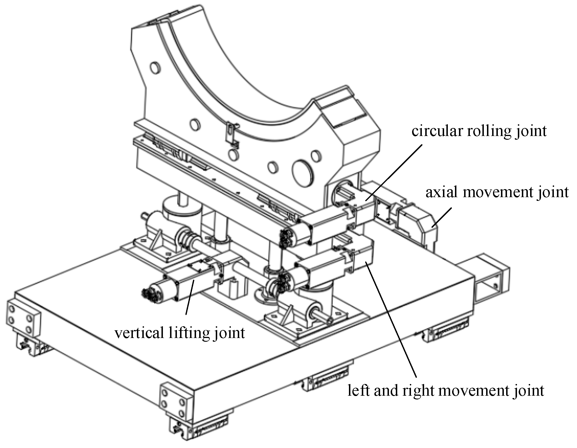
The structure details of the right arm are given in Figure 2. The axial movement joint, vertical lifting joint and circumferential rolling joint are seen. Thus, there are six degrees of freedom for the dual arm: pitch, yaw, roll, lifting, front and rear. The axial movement joint is driven by the motor–gear–rack system, and the left movement joint and right movement joint are driven by the motor-screw systems. The vertical lifting joint is driven by the motor–spiral elevator for the lifting, and the circular rolling joint is driven by the motor–gear transmission system. There is an arc-shaped structure for the circular rolling joint, and the special rubber is used to increase the friction force among the workpieces.
On the basis of the above arm construct, trajectory planning is needed for the cabin docking. There are two steps for the trajectory planning: trajectory generation and trajectory optimization. The precondition for trajectory planning is provided by the former, while the trajectory performance is improved by the latter [3]. The trajectory is generated by the discrete path points, and the points are obtained by polynomial functions, parabolic functions or B-spline curve functions [4,5,6,7,8]. Therefore, in order to confirm the optimal trajectories, the multi-objective trajectory optimization algorithm has become an important aspect [9]. And some parameters are used for the multi-objective optimization parameters, such as the minimum execution time, minimum energy consumption and minimum disturbance. Firstly, an improved immune clone selection algorithm was proposed by Chen et al. [10]. In this algorithm, a multi-objective model for trajectory optimization was established using the total motion time, total energy consumption and actuator thrust. The trajectory was generated using a fifth-order B-spline curve, and the improved immune clone algorithm was used for the trajectory optimization. Lan et al. discussed a multi-objective trajectory planning method for collaborative robots [11]. Based on the collaborative kinematic model, the joint trajectories were constructed from the B-spline curves. The multi-objective particle swarm optimization algorithm was used for the Pareto optimal solution of the time-energy jump optimal trajectories. Then, the most suitable solution is selected using the normalized weighting function. A novel optimal trajectory planning method was constructed by Wang et al. [12]. A trajectory was created with fifth-order polynomials and cubic Bézier curves. The genetic operators were used for optimizing the travel time and torque functions, such as Rank-based Group Selection (RGS), Direction-based Crossover (DBX) and Adaptive Precision Controlled Mutation (APCM). Then, in virtue of Hermite cubic interpolation, the polynomial was used for the trajectory process of space species [4].
Compared with other algorithms, the Cuckoo Search (CS) algorithm is a new swarm optimization algorithm, which is heuristic and intelligent. There are also strong global search capabilities and fewer parameter settings [13,14,15,16]. Thus, a multi-objective Cuckoo Search Algorithm (MOCS) was proposed by Yang et al. [17]. The novel multi-objective improved Cuckoo optimization algorithm was built by Azizipanah et al. [18]. A set of non-dominated points were defined for the optimization problems. This algorithm was applied in the multi-objective static and dynamic optimization scheduling of a thermal-electric system, where the environmental objective was inconsistent with the economic objective. For the automotive sequencing problem of a mixed-model assembly line, the multi-objective Cuckoo Search algorithm was proposed by Wang et al. [19]. The algorithm was based on the record matrices. More factors were considered, such as part usage variation, workstation workload variation, idle time, overload time and model change cost. Meanwhile, two search strategies were also given, and the local and global search capabilities were enhanced. Later, the trajectory planning problems were solved by the Cuckoo Optimization Algorithm (COA), Cuttlefish Algorithm (CFA), Seagull Optimization Algorithm (SOA) and Tunicate Swarm Algorithm (TSA) [20].
From the above studies, less attention is paid to the optimization algorithm of the dual-arm robot. Therefore, on the basis of a modified Cuckoo Search algorithm, a multi-objective trajectory planning method is proposed. The trajectory is generated using a fifth-order B-spline curve, and the total consumption time and joint impact are minimized by the objective functions. The normalization comprehensive evaluation method is used for the solutions in the Pareto non-dominant, and the most comprehensive optimal solution is selected. The relative results are verified by the experiments. And the subsequent organization is given based on the above method. In Section 2, a kinematics model of the dual-arm robot is established. The trajectory is planned by the B-spline curve in Section 3. Later, a modified Cuckoo Search algorithm is proposed by the objective function and comprehensive optimal solution method, which can be found in Section 4. From Section 5, the effectiveness of the algorithm is verified by the simulation. The confirmatory experiment is given in Section 6. The conclusions are seen in Section 7.

2. Kinematic Analysis of Cabin Docking Dual-Arm Robot

2.1. Forward Kinematic Model

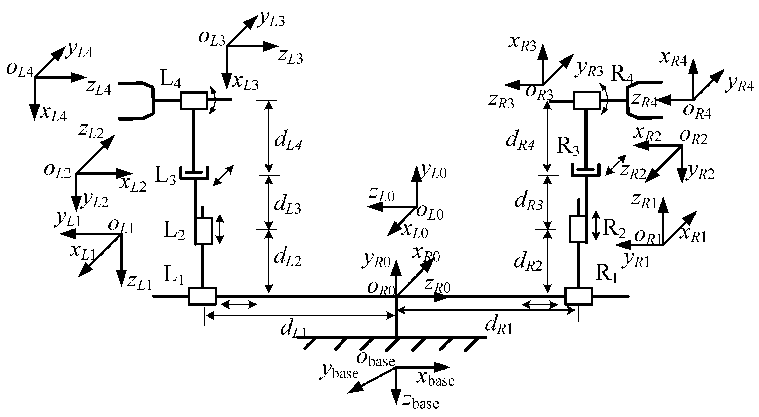
According to the organization, a simplified model of a dual-arm robot is constructed, and the relative coordinate systems are given in Figure 3. The relationship between the adjacent links of a dual-arm robot is established through the Denavit–Hartenberg (D-H) method. The base coordinate system is represented by Obasexbaseybasezbase. Two robotic arm coordinate systems OL0xL0yL0zL0 and OR0xR0yR0zR0 are established at the middle position. The axial movement joint, vertical lifting joint, left and right movement joint and circumferential rolling joint of the left robotic arm are, respectively, established with OL1xL1yL1zL1, OL2xL2yL2zL2, OL3xL3yL3zL3 and OL4xL4yL4zL4. The D-H parameters of the cabin docking dual-arm robot are given in Table 1.
On the basis of the D-H method, the terminal position matrix of the left robotic arm is as follows:
base L 4 T = base L 0 T L 0 L 1 T L 1 L 2 T L 2 L 3 T L 3 L 4 T = 0 0 1 d L 1 sin ( θ L ) cos ( θ L ) 0 d L 3 cos ( θ L ) sin ( θ L ) 0 d L 2 0 0 0 1
where b a s e L 0 T is the transition matrix from Obasexbaseybasezbase to OL0xL0yL0zL0, L 0 L 1 T is the transition matrix from OL0xL0yL0zL0 to OL1xL1yL1zL1, L 1 L 2 T is the transition matrix from OL1xL1yL1zL1 to OL2xL2yL2zL2, L 2 L 3 T is the transition matrix from OL2xL2yL2zL2 to OL3xL3yL3zL3, and L 3 L 4 T is the transition matrix from OOL3xL3yL3zL3 to OL4xL4yL4zL4.
Similar methods are used for the right robotic arm, and the terminal position matrix can be obtained as follows:
base R 4 T = 0 0 1 d R 1 sin ( θ R ) cos ( θ R ) 0 d R 3 cos ( θ R ) sin ( θ R ) 0 d R 2 0 0 0 1

2.2. Inverse Kinematics Model

The inverse kinematics model of the dual-arm rotor can be solved with the formula Paul inverse transformation method. The pose matrix equation of the right robotic arm is
base R 4 T = n R x o R x a R x p R x n R y o R y a R y p R y n R z o R z a R z p R z 0 0 0 1
According to Equations (2) and (3), the forward kinematics formula for the right robotic arm can be obtained as follows:
p R x = d R 1 p Ry = d R 3 p Rz = d R 2 y a w R = θ R
The same method is also used for the left robotic arm, the forward kinematics equation is
p Lx = d L 1 p Ly = d L 3 p Lz = d L 2 y a w L = π + θ L
In view of the mapping relationship of Equations (4) and (5), the inverse kinematics transformation formulas of the right robotic arm and the left robotic arm can be established as follows:
d R 1 = p R x d R 3 = p Ry d R 2 = p Rz θ R = y a w R
d L 1 = p Lx d L 3 = p Ly d L 2 = p Lz θ L = y a w L

3. Trajectory Planning Method Based on B-Spline Interpolation

3.1. Trajectory Planning Scheme

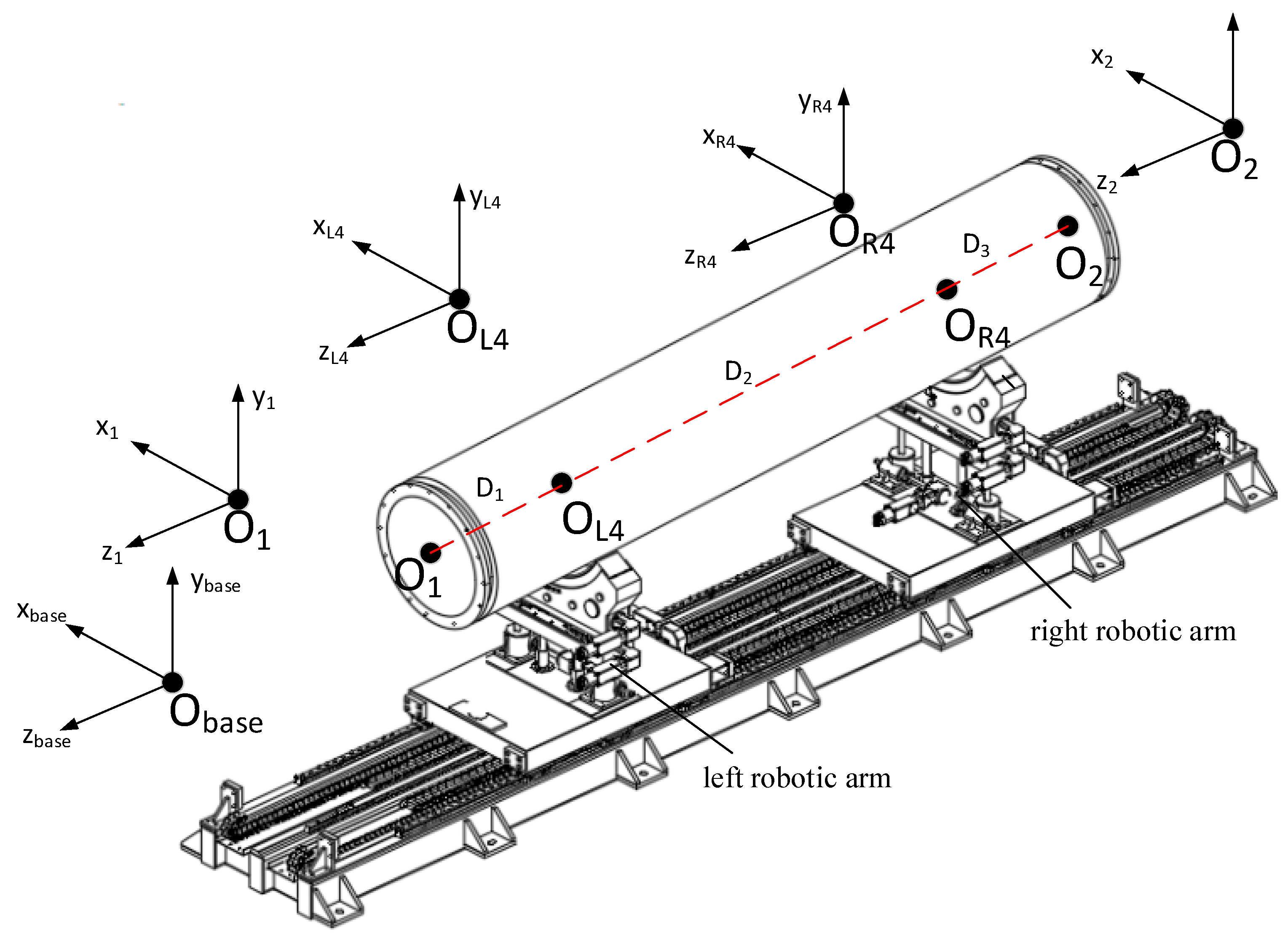
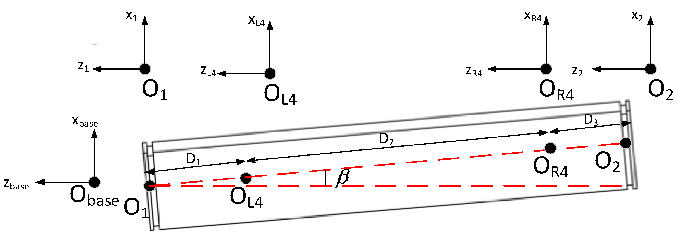
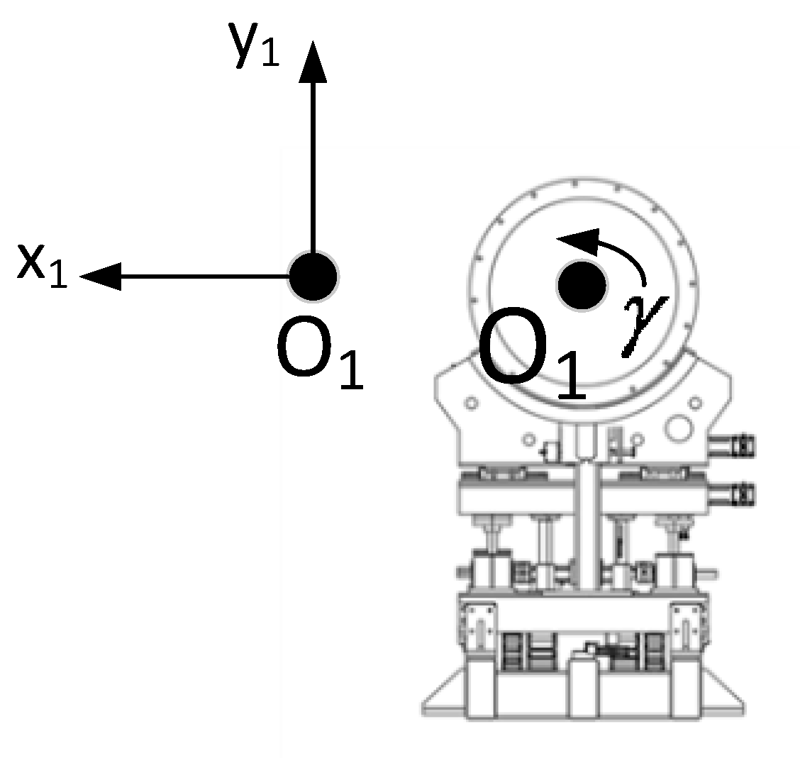
In Figure 4, in order to analyze the attitude adjustment process of the dual-arm robot, the left center coordinate system O1x1y1z1 of the cabin workpiece is established, and the right center coordinate system is O2x2y2z2. The axial movement direction of the cabin docking robot is defined as the Z-axis direction. The movement direction of the cabin docking robot is defined as the X-axis direction. The movement direction of the cabin docking robot along the vertical lifting joint is defined as the Y-axis. The distance between OL4xL4yL4zL4 and O1x1y1z1 is D1, the distance between OR4xR4yR4zR4 and O2x2y2z2 is D3, and the distance from OL4xL4yL4zL4 to OR4xR4yR4zR4 is D2. According to the established coordinate system, the Pitch angle α, the Yaw angle β and the Roll angle γ are defined, which can be found in Figure 5. As shown in Figure 4, the dashed line is the cabin workpiece axis.
For analyzing the relationship between the workpiece and the cabin docking robot, there are four situations: the initial equilibrium position, 0° pitch angle, 0° yaw angle and 0° roll angle. Their detailed descriptions are as follows:
(1)
Initial equilibrium position
In the actual production process, it is generally required that the cabin docking robot is in the balanced spatial posture. O1x1y1z1, OL4xL4yL4zL4, O2x2y2z2 and OR4xR4yR4zR4 are in a straight line. The pitch angle α, the yaw angle β and the roll angle γ are set as 0°, as shown in Figure 6. The positional relationship in the z direction is
z 1 z L 4 2 = D 1 2 z L 4 z R 4 2 = D 2 2 z R 4 z 2 2 = D 3 2
(2)
0° pitch angle
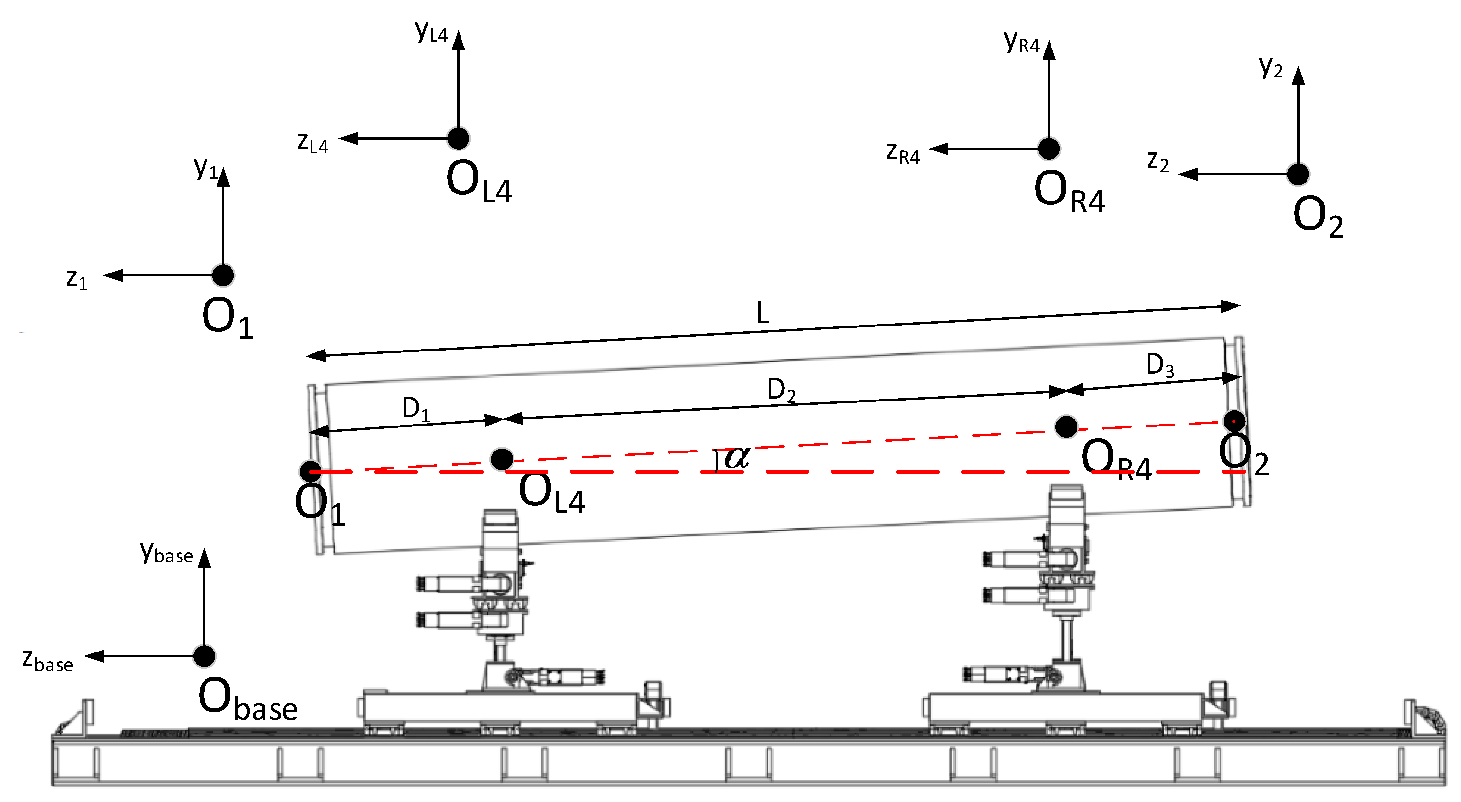
Due to frictional force between the cabin docking robot and the workpiece, the vertical lifting of the docking robot is limited, and the value is often ±50 mm. When the pitch angle of the workpiece is changing, the end of the docking robot still contacts with the workpiece. Therefore, O1x1y1z1, OL4xL4yL4zL4, O2x2y2z2 and OR4xR4yR4zR4 are also on a straight line. As seen in Figure 7, the positional relationship of the coordinate system is
y 1 y L 4 2 + z 1 z L 4 2 = D 1 2 y L 4 y R 4 2 + z L 4 z R 4 2 = D 2 2 y R 4 y 2 2 + z R 4 z 2 2 = D 3 2
As seen in Figure 7, there are two dashed lines in red, one is the current cabin workpiece axis, the other is the cabin axis at the balance position, and the angle between the two lines is attitude angle. The relationship between the pitch angle and the coordinate system parameters is
sin α = y R 4 y L 4 D 2
(3)
0° yaw angle
The same method used for the pitch angle is also used for the yaw angle. From Figure 8, the positional relationship of the coordinate system is
x 1 x L 4 2 + z 1 z L 4 2 = D 1 2 x L 4 x R 4 2 + z L 4 z R 4 2 = D 2 2 x R 4 x 2 2 + z R 4 z 2 2 = D 3 2
The relationship between the pitch angle and the coordinate system parameters is
sin β = x R 4 x L 4 D 2
(4)
0° roll angle
In view of the workpiece, the positional relationships of various coordinate systems are not affected by the changing roll angle. Thus, all the coordinates are also on a straight line, which can be seen in Figure 9. However, in consideration of the bolt connection between the workpieces, the roll angle is also adjusted with a slight change in the cabin space pose.
Based on the above analysis, the adjustment processes for the position and attitude of the workpiece are independent of each other. It is assumed that the trajectory for the end of the left robotic arm is KL4(xL4(t), yL4(t), zL4(t)), and the end of the right arm is KR4(xR4(t), yR4(t), zR4(t)). The first formula for the trajectory planning scheme is
x L 4 t x R 4 t 2 + y L 4 t y R 4 t 2 + z L 4 t z R 4 t 2 = D 2 2
In Equation (13), on the basis of the motion trajectory for the left robotic arm, the spatial position is aligned, the end of the right robotic arm is changed with the action of the left robotic arm. The distance from the end of the left robotic arm to the end of the right robotic arm is constant. In addition to participating in spatial position adjustment, the right robotic arm is also used to adjust the posture of the cabin segment. Thus, the motion trajectory of the right robotic arm can be divided into two parts: KR41(xR41(t), yR41(t), zR41(t)) and KR42(xR42(t), yR42(t), zR42(t)). The relationship is as follows:
K R 4 x R 4 t , y R 4 t , z R 4 t = K R 4 1 x R 4 t , y R 4 t , z R 4 t + K R 4 2 x R 4 t , y R 4 t , z R 4 t
where KR41(xR41(t), yR41(t), zR41(t)) is used to follow the action of the left robotic arm, while KR42(xR42(t), yR42(t), zR42(t)) reflects the attitude change of the cabin segment, and the relative formula is given as follows:
x R 4 2 t = x L 4 t + D 2 cos α t cos β t y R 4 2 t = y L 4 t + D 2 cos α t sin β t z R 4 2 t = z L 4 t + D 2 cos α t
where α(t) and β(t) represent the pitch angle and yaw angle trajectory of the workpiece, respectively.

3.2. B-Spline Curve Construction

The B-spline curves are widely used for the robot trajectory planning due to the advantages, such as derivative continuity, piecewise processing and local support. The first and second derivatives of the B-spline curve are both continuous, which can meet the requirements of trajectory planning. The definition of a k-th degree B-spline curve is as follows:
p u = i = 0 n c i N i , k u
where ci is the control point, and Ni,k(u) is a k-th degree B-spline basis function. There are several approaches for representing B-Spline base functions, which are often defined as the de Boor–Cox recursion formula [21,22]. The order of the B-spline curve is selected as five, the number of intermediate control points is five, three expresses the endpoint repetitions of control points, and the endpoint repetitions of node vectors is six. Then, the total number of control points is 11, and the element number in the node vector is 17. The initial and final pose of the cabin segment is expressed as follows:
p o = p o x , p o y , p o z , p o α , p o β , p o γ p e = p e x , p e y , p e z , p e α , p e β , p e γ
There are three repetitions for the control points at the beginning and end positions:
d 0 p = d 1 p = d 2 p = p 0 d 8 p = d 9 p = d 10 p = p e
Therefore, the vector can be represented as
d = d 0 p , d 1 p , d 2 p , d 3 p , d 4 p , d 5 p , d 6 p , d 7 p , d 8 p , d 9 p , d 10 p
The time nodes of the initial and final pose points have a duplicate degree of six. Therefore, the time node vector can be represented as follows:
t = 0 , 0 , 0 , 0 , 0 , 0 , t 1 , t 2 , t 3 , t 4 , t 5 , t 6 , t 6 , t 6 , t 6 , t 6 , t 6
The B-spline curve of pose motion trajectory is differentiated as velocity, acceleration and jerk. The relative expression is as follows:
v t = i = 0 9 d i v N i , 4 t i = 0 , 1 , , 9 a t = i = 0 9 d i a N i , 3 t i = 0 , 1 , , 8 j t = i = 0 9 d i a N i , 2 t i = 0 , 1 , , 7
The sequence of control points are
d i v = k d i + 1 p d i p t i + k + 1 p t i + 1 p i = 0 , 1 , , 9 d i a = k 1 d i + 1 v d i v t i + k v t i + 1 v i = 0 , 1 , , 8 d i j = k 2 d i + 1 a d i a t i + k 1 a t i + 1 a i = 0 , 1 , , 7
k is the order of the position B-spline curve, and the value is five. The node vector corresponding to each control point is as follows:
t v = 0 , 0 , 0 , 0 , 0 , t 1 , t 2 , t 3 , t 4 , t 5 , t 6 , t 6 , t 6 , t 6 , t 6 t a = 0 , 0 , 0 , 0 , t 1 , t 2 , t 3 , t 4 , t 5 , t 6 , t 6 , t 6 , t 6 t j = 0 , 0 , 0 , t 1 , t 2 , t 3 , t 4 , t 5 , t 6 , t 6 , t 6
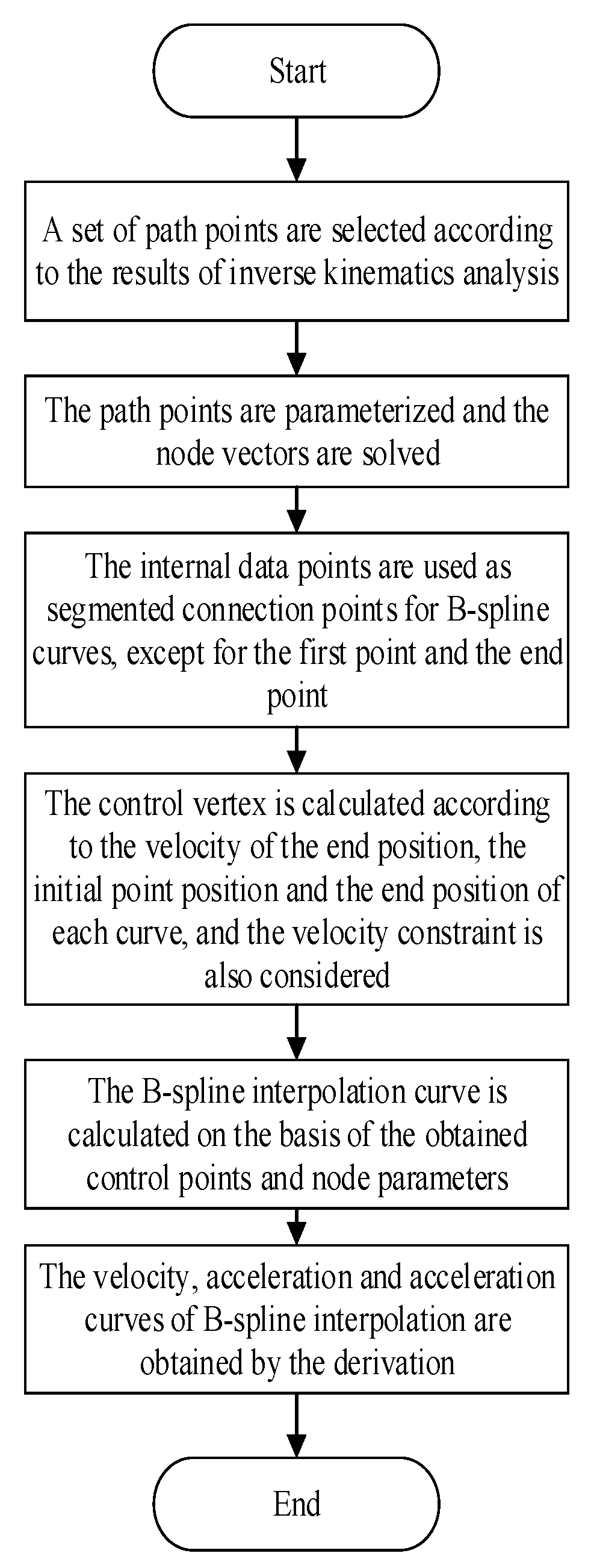
According to Equations (21)–(23), the velocity, acceleration and jerk curves can be computed. The trajectory planning process of the fifth degree B-spline curve is shown in Figure 10.

4. The Modified Multi-Objective Cuckoo Search Algorithm

4.1. The Objective Function and Comprehensive Optimal Solution

During the docking process of the workpieces, the docking time should be shortened, which can ensure the efficiency. Therefore, the total consumption time of the dual-arm robot is selected as the first objective evaluation function:
S 1 = T = t i
where ti is the node vector for the parametric variable of the B-spline.
In addition to the high work efficiency, the stability is also very important. However, the impacts are often generated when the dual-arm robot is working. In order to keep the motion trajectory smoother and more stable, the impact must be contained within a small range. Therefore, the second objective evaluation function is defined as follows:
S 2 = j = 1 N 1 T 0 T q j t 2 d t
where q j t refers to the jerk of the j-th joint.
After the objective evaluation functions are confirmed, the comprehensive optimal solution should also be given. However, the comprehensive optimal solution is closely linked to the multi-objective optimization. The significant feature of multi-objective optimization is that each objective function is mutually constrained. If the value of one objective function is optimal, the performance of other objective functions is often lost. In the feasible solution set of multi-objective optimization problems, there is no traditional absolute optimal solution, which can ensure that all objective functions are the optimal value simultaneously. Then, it is often determined by the dominance relationship, and the non-dominated solution is considered as the final effective solution, which is also called as the Pareto optimal solution [23]. The normalization of various indicators is used for the Pareto optimal solution. In this method, all the indicators are normalized, the influence of units is eliminated, and a comprehensive evaluation value for the non-dominated solutions can be obtained. Each set of Pareto solutions is calculated for the satisfaction indicators of all objective functions. And the satisfaction indicator is minimized as the optimal solution, which is defined as follows:
δ = 1 m i = 1 m w i f i max f i f i max f i min
where m represents the number of objective functions, and fimax and fimin are the maximum and minimum values of the i-th objective function. w = [w1, w2] represents the weight coefficient, which serves as a trade-off criterion between time optimality and impact optimality. By adjusting the ratio between w1 and w2, different weights for time and impact can be achieved.

4.2. Traditional Multi-Objective Cuckoo Search Algorithm

The Cuckoo Search algorithm (CS) is an optimization algorithm, and it is used to simulate the special habit of cuckoo laying eggs. The Multi-Objective Cuckoo Search algorithm (MOCS) is an improvement of the CS algorithm, where a single objective function is replaced by multiple conflicting objectives for the global search [24]. The search path and location update equations of the algorithm are as follows:
X i ι + 1 = X i ι + α L e vy β
where X i ι + 1 represents the location of the i-th nest in generation t + 1, α > 0 denotes the step size, X i ι is the random location of the nest in generation t, and denotes the point-to-point multiplication. L e vy β is the randomized step size, which can be calculated as
L e vy ~ u = t 1 β , 0 β 2
In MOCS, the complete L e vy equation is as follows:
α 0 x j ( t ) x i ( t ) levy ( β ) ~ 0.01 u | v | 1 / β ( x j ( t ) x i ( t ) )
where u and v are normally distributed.

4.3. Modified Multi-Objective Cuckoo Search Algorithm

Compared with other multi-objective optimization algorithms, there are some advantages of the MOCS algorithm, such as few parameters and strong optimization ability. However, the drawbacks are not ignored, such as slow convergence speed in the later period and uneven distribution of optimal solutions. Aiming at the above drawbacks, a modified multi-objective Cuckoo algorithm (IMOCS) is proposed for chaotic initialization of the population. The diversity and uniformity of the initial population are ensured, the adaptive step size is introduced during the Levi flight process, which can effectively develop the algorithm’s global and local optimization capabilities, and the improvement plan will be described in detail.

4.3.1. Improvement of Initial Population Generation Method

In the traditional MOCS algorithm, the initial population is generated randomly, and the equation is as follows:
X i 0 ~ N 0 , 1
where X i 0 represents the position of the i-th bird’s nest at the initial moment.
The random initialization may lead to an uneven population distribution, a large number of poor solutions are generated, and the convergence speed of the algorithm becomes slower. Thus, the characteristics of chaos principles are integrated, the population diversity is improved without losing individual randomness, a foundation is provided for a further effective global search. Bernoulli chaotic mapping is used to initialize the population for chaos, and its expression is
Z k + 1 = Z k / 1 ρ Z k 0 , 1 ρ Z k 1 + ρ / ρ Z k 1 ρ , 1
where Zk represents the current value of the chaotic sequence generated in the k-th generation, and ρ is the control parameter.
The steps of chaos initialization are as follows:
Step 1: For the locations of S nests in n-dimensional space, a random n-dimensional vector is generated as the location of the first nest. Among them, y i 0 , 1 , 1 i d .
Step 2: each dimension of Y1(0) is iterated for S-1 times, S-1 chaotic variables Y2(0), …, YS-1(0), YS(0) are generated.
Step 3: the positions of the nests in the solution space are generated by using the S chaotic variables, which is described as
x i d = L d + y i d U d L d
where Ud and Ld represent the upper and lower bounds of the d-th dimension of the search space.

4.3.2. Improvement of Step Size in Cuckoo Algorithm

There is a fixed step size factor α0 in the traditional cuckoo algorithm, the adaptive adjustment of step size cannot be achieved during the optimization process, and the convergence speed of the algorithm is slow. In the optimization process, if the step size factor α0 is large, the algorithm has strong exploration ability, but the high-precision global optimal solutions cannot be obtained. If the step size factor α0 remains small, the algorithm will require more iterations for target accuracy. In addition, biological heuristic algorithms originate from the characterization of natural biological behavior habits, and there is significant randomness.
In response to the above shortcomings, an adaptive Levi flight mechanism is used for the global search, and the Levy flight step size continuously decreases with iteration. The improved algorithm has a larger step size factor in the early stage of optimization, thereby the search space in the early stage of the algorithm is expanded, and the global search ability is improved. During the optimization process, the step size is reduced, and the local search performance of the algorithm is improved. The step size updating equation is shown as follows:
α 0 = α max 1 i t e r 1 M a x i t e r 2
where αmax represents the maximum step length, iter denotes the current iteration number, and Maxiter is the total iteration number.

4.4. Flowchart of Trajectory Optimization Algorithm

Firstly, the parameterized B spline curve is used to express the trajectory. According to the optimization objective and the range of adjusting mechanism parameters, the optimization algorithm adaptation functions and constraints are constructed to establish the multi-objective optimization trajectory. The multi-objective optimization algorithm is used for the set of Pareto optimal solutions, and the index normalized evaluation method is given for the comprehensive optimal solution. The relative flowchart is shown in Figure 11.

5. Simulation Analysis

To verify the effectiveness of the multi-objective trajectory optimization algorithm, the trajectory planning simulation is conducted on the docking robot. At the same time, in order to verify the modified multi-objective cuckoo search algorithm, the NSGA-II algorithm, MOPSO algorithm, MOCS algorithm and IMOCS algorithm are, respectively, used in the simulation experiments, comparative simulation experiments are carried out, and the experimental results are analyzed.

5.1. Parameter Configuration

The start point and end point of the position for the simulation process are set as
P o = [ 775 , 35 , 1315 , 0.2 , 0.2 , 190 ] P e = [ 745 , 5 , 1515 , 0 , 0 , 180 ]
The elements from left to right in the vector are the X-axis position, the Y-axis position, the Z-axis position, the pitch angle, the yaw angle and the roll angle. The parameters of a docking robot are selected as the constraint conditions, and the relative value is given in Table 2.

5.2. Results and Discussion

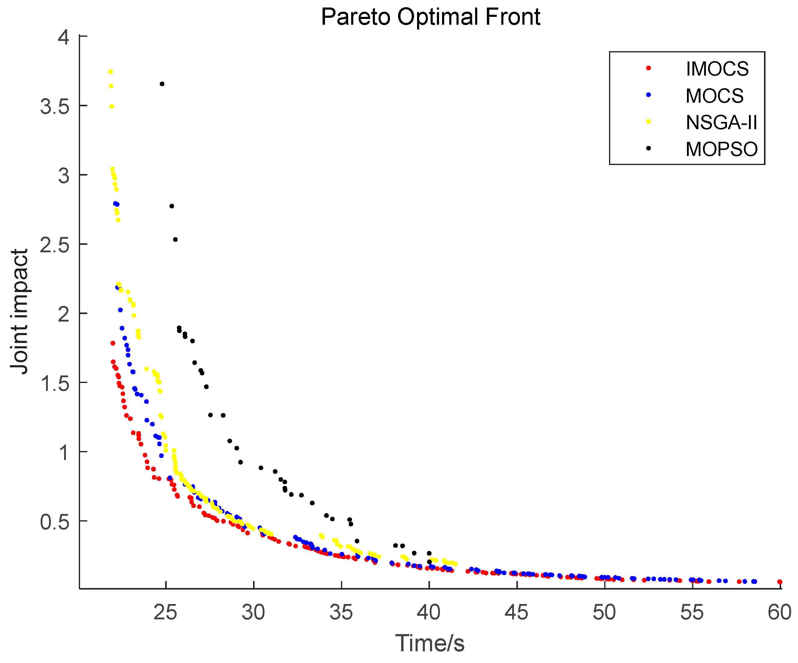
Compared with the performance of different Multi-Objective Evolutionary Algorithms (MOEAs), the indicators are divided into counting indicators, convergence indicators, diversity indicators and comprehensive indicators [25]. The counting index is used to count the number or proportion of non-dominated solutions, which is based on the Overall Non-dominated Vector Generation (ONVG) [26]. The convergence index is chosen as the Generational Distance (GD) [27], and the average distance from the solution to the closest reference point is calculated. The diversity selection spatial indicator spacing (SP) [28] is used to reflect the diversity of the optimal solution in the spatial distribution. To ensure the rationality of the simulation, the population size is set to 150, and after 100 iterations, the Pareto front is shown in Figure 12.
(1) Comparing the number of non-dominated solutions, the non-dominated solutions of the NSGA-II algorithm, the MOPSO algorithm, the MOCS algorithm and the IMOCS algorithm are 150, 36, 133 and 150, respectively. Therefore, in terms of the number for non-dominated solutions, the IMOCS algorithm is superior to the MOPSO and MOCS algorithms, and it is comparable to the NSGA-II algorithm.
(2) Comparing the convergence of non-dominated solutions, the GD values of the NSGA-II algorithm, the MOPSO algorithm, the MOCS algorithm and the IMOCS algorithm are 0.0065, 0.0220, 0.0041 and 0.0019, respectively. As a result, the convergence of the IMOCS algorithm is better.
(3) Comparing the spacing of non-dominated solutions, the SP values of the NSGA-II algorithm, the MOPSO algorithm, the MOCS algorithm and the IMOCS algorithm are 0.0049, 0.0420, 0.0064 and 0.0037, respectively, so the spacing of the IMOCS algorithm is better.
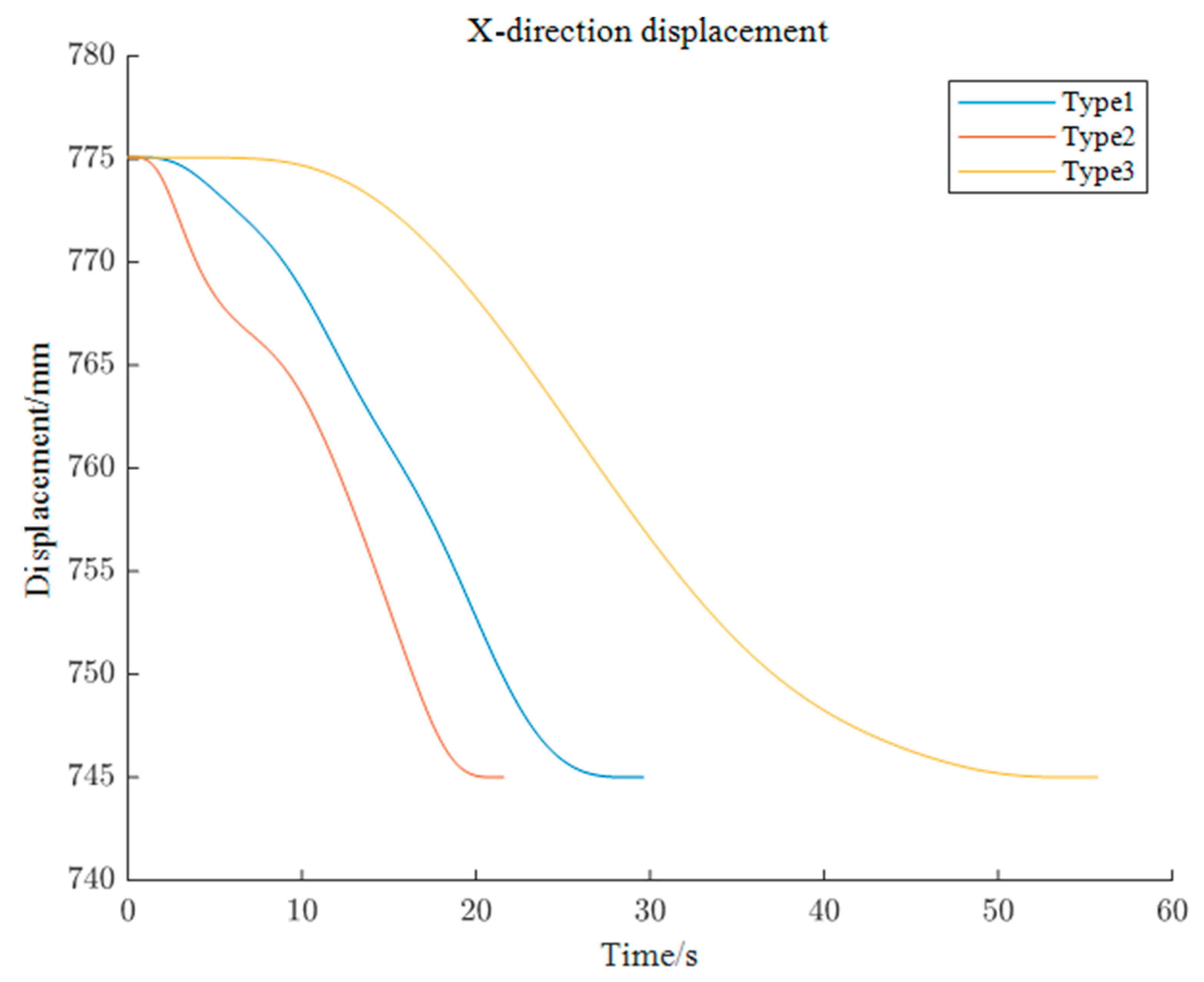
In order to analyze the time shock distribution relationship in the non-dominated solution set more intuitively, 11 sets of solutions are uniformly selected from the non-dominated solution set obtained by the IMOCS optimization algorithm, as shown in Table 3. The total time of cabin docking is increasing from 21.5743 s to 59.5678 s. With the increasing total time, the joint impact decreases from 3.9448 to 0.0753. The normalization method is used to solve the optimal solutions in these 11 groups. The weight coefficients are set according to Equation (26), which is shown in Table 4.
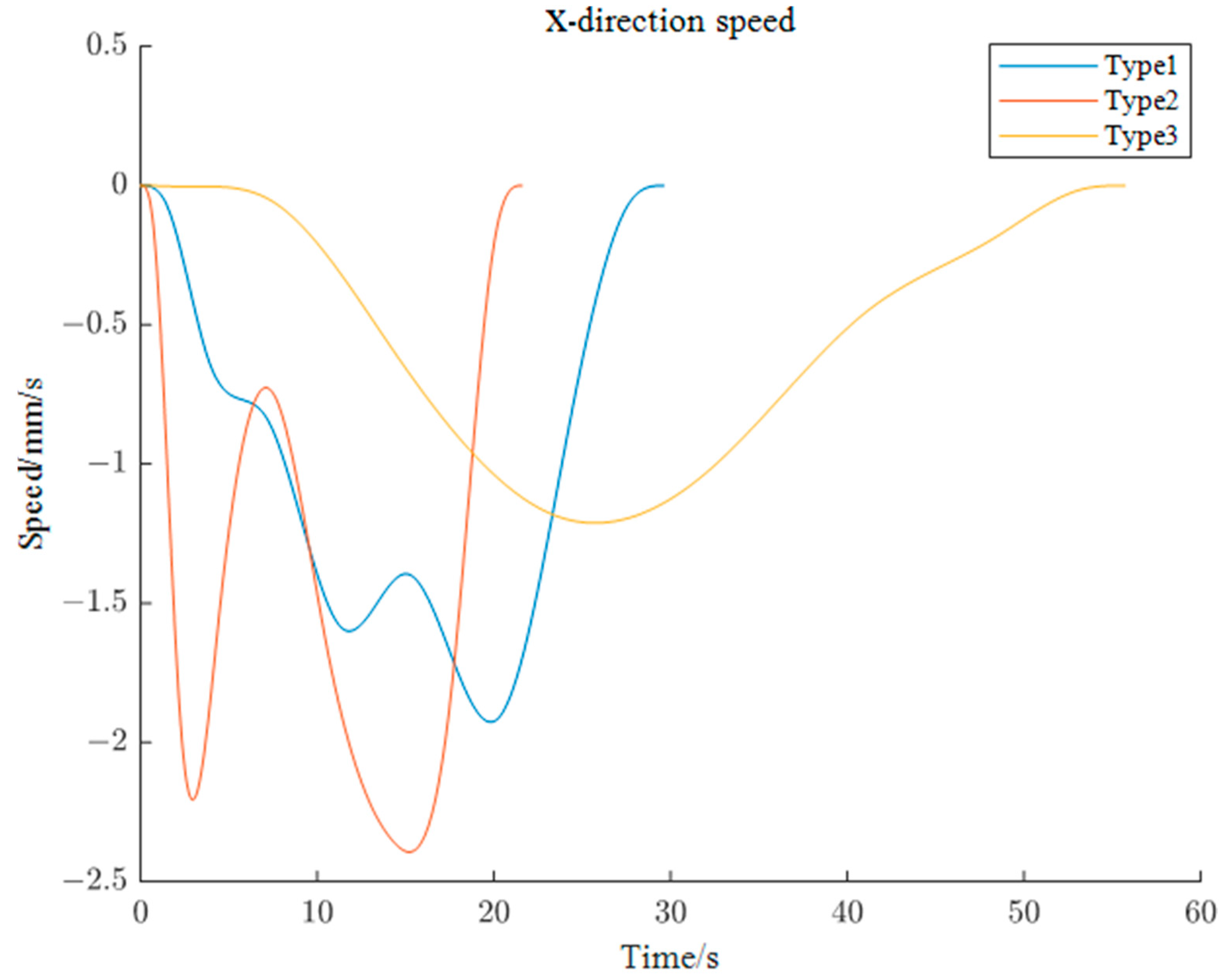
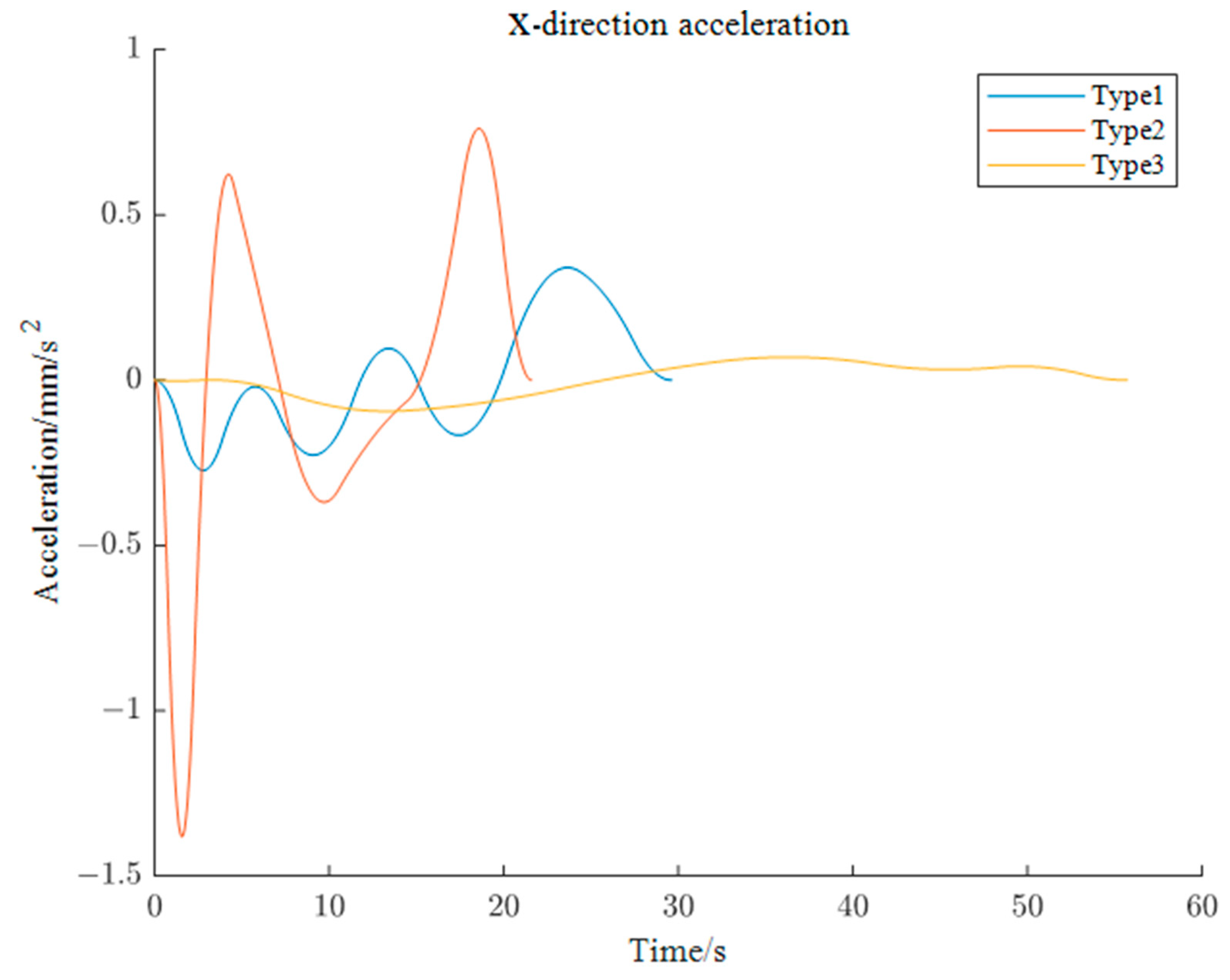
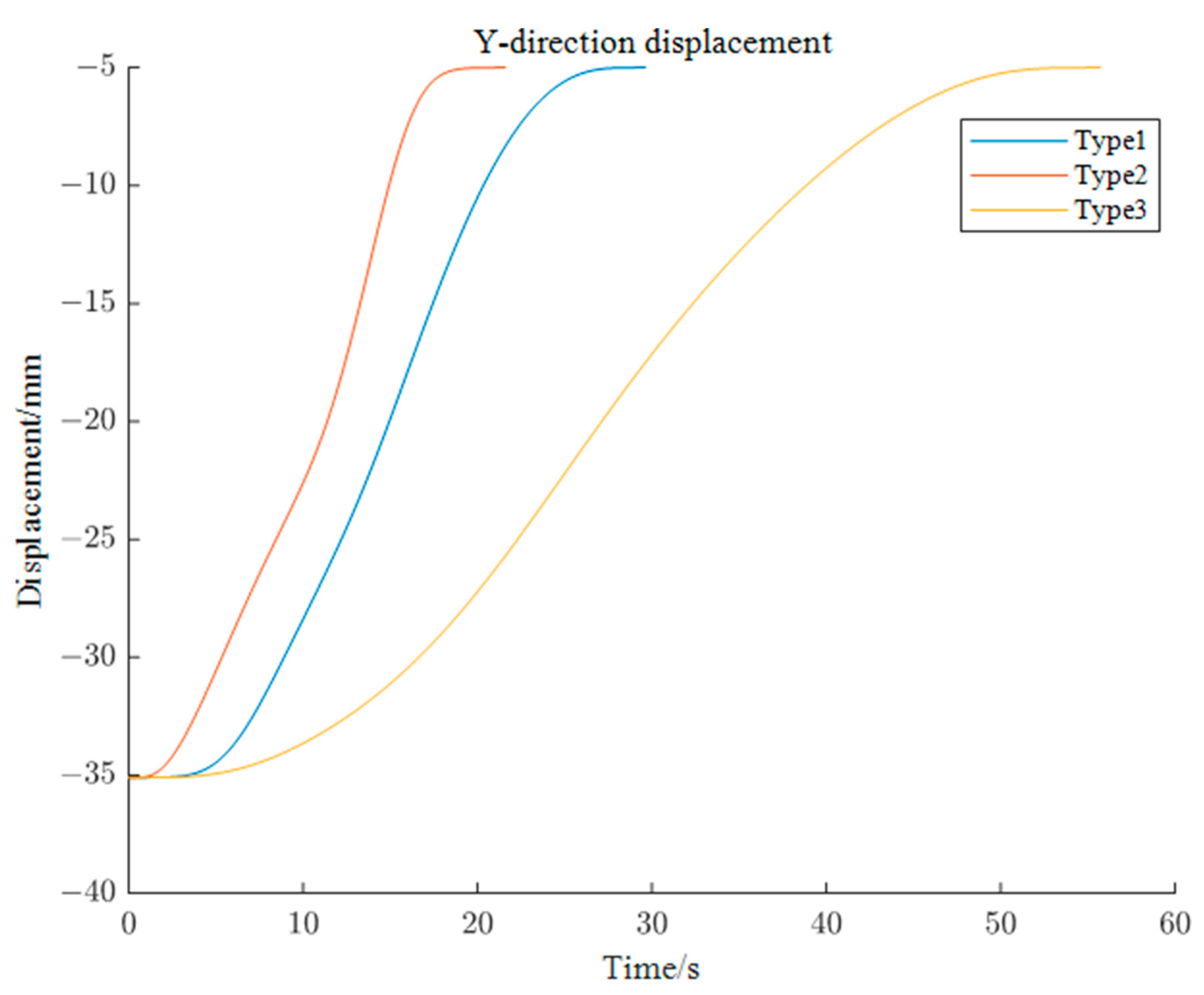
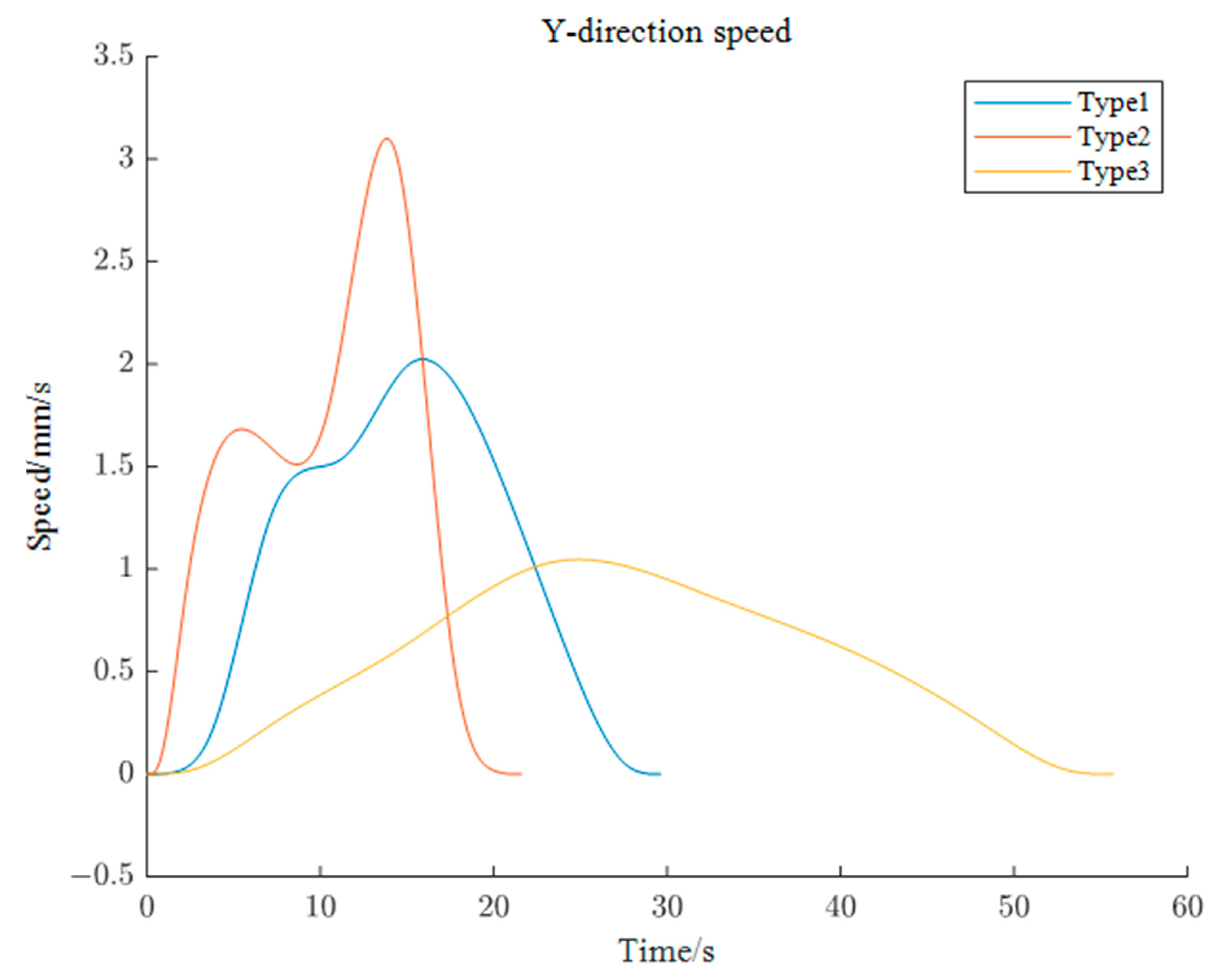
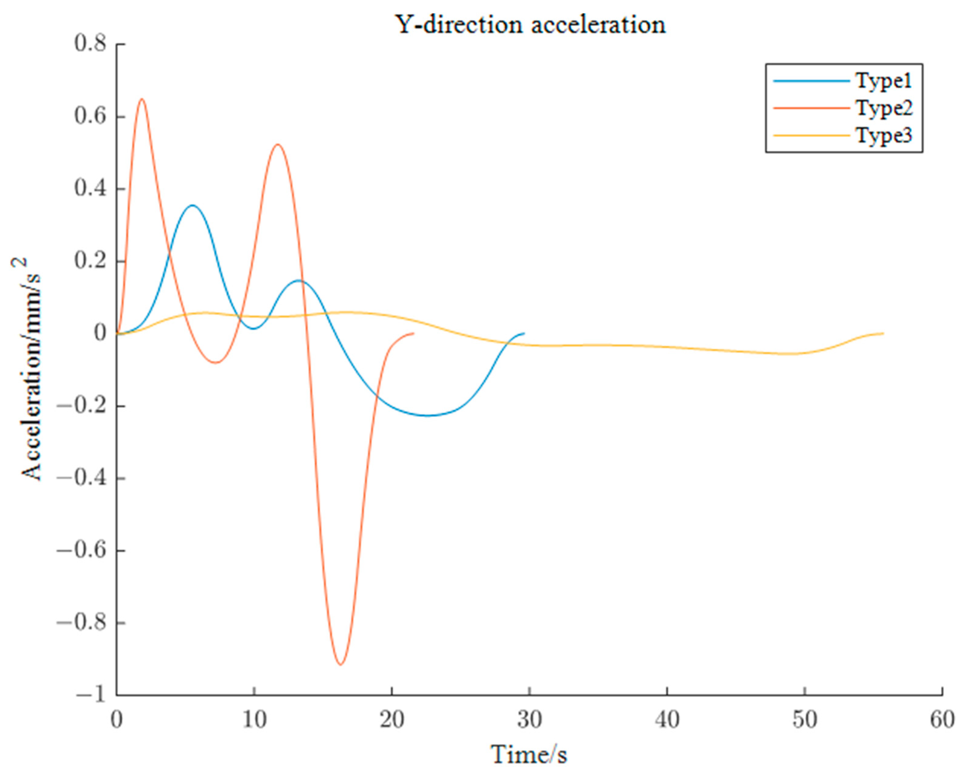
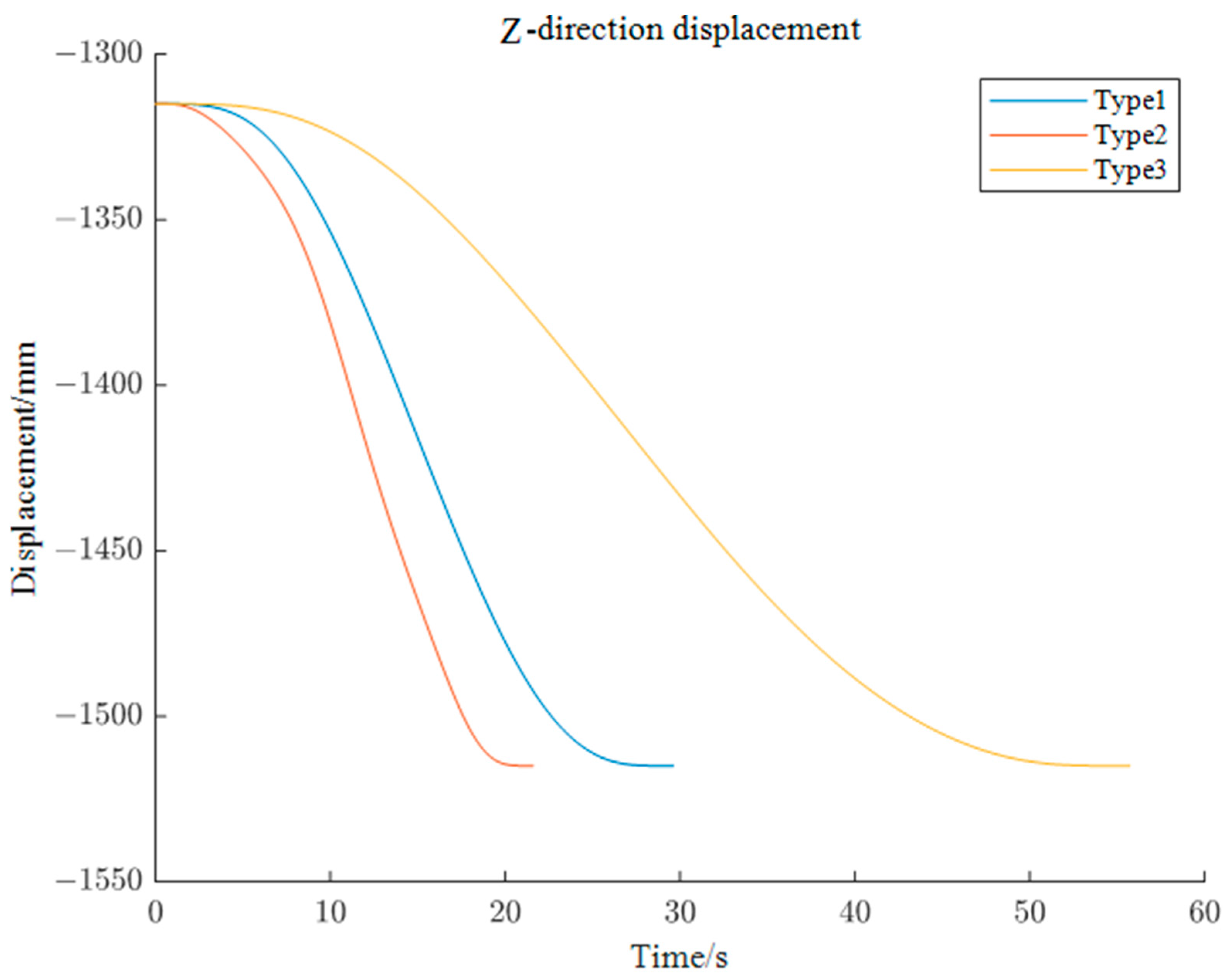
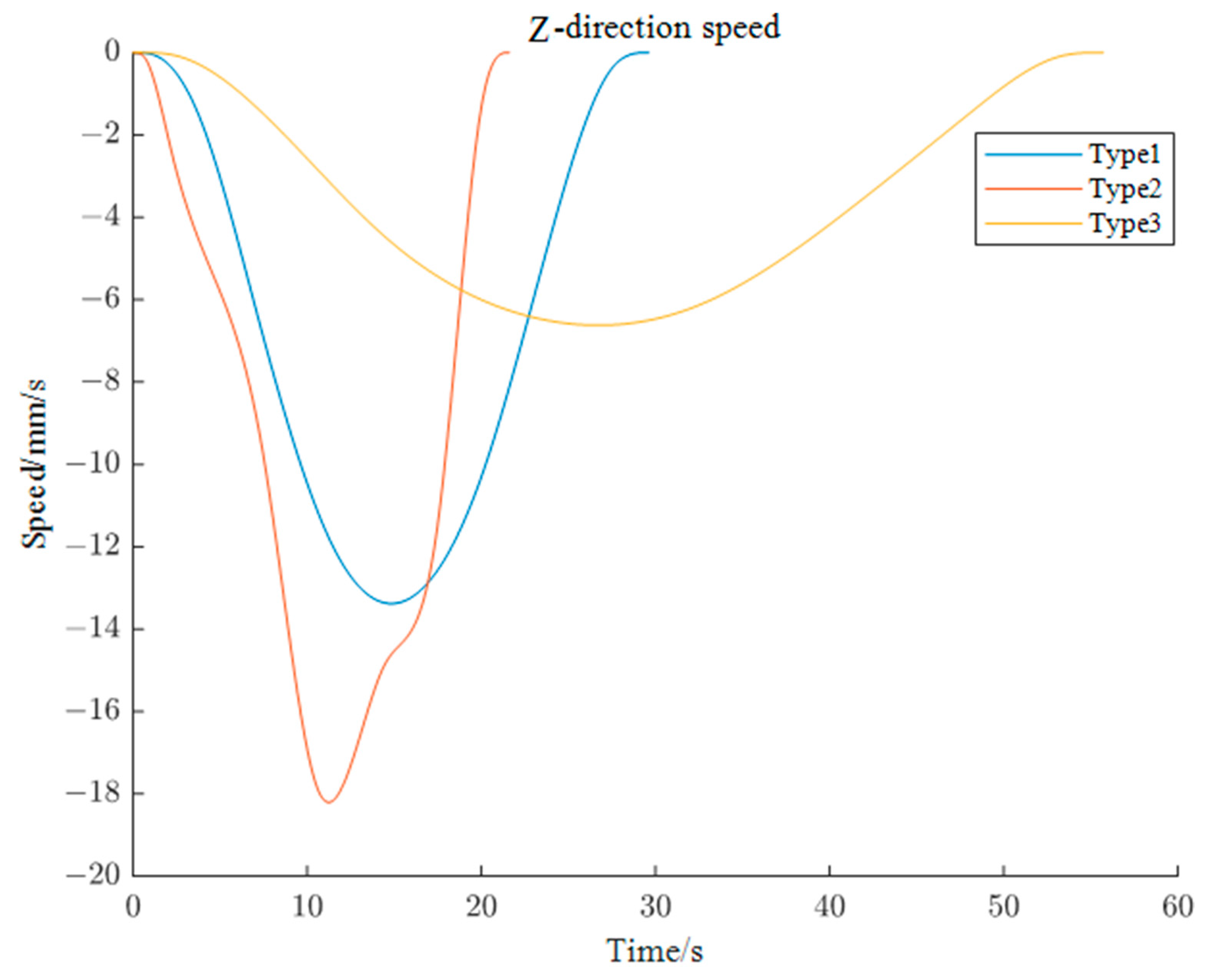
From Table 4, three coefficient types are set using the normalized evaluation method. Type 1 is a weight coefficient [w1, w2] = [1, 1], and the comprehensive optimal solution of the total time and joint impact objective functions in the non-dominated solution are selected. Type 2 is a weight coefficient [w1, w2] = [0, 1], and the solution with the smallest total time among non-dominated solutions is selected. Type 3 is the weight coefficient [w1, w2] = [1, 0], and the solution with the smallest joint impact among non-dominated solutions is selected. The corresponding solutions can be obtained from Table 4 based on the selection method of these solutions. Then, the simulations are made for the end X-axis motion trajectory of the left robotic arm, the end Y-axis motion trajectory of the left robotic arm, and the end Z-axis motion trajectory of the left robotic arm.

5.2.1. Simulation of X-axis End Motion Trajectory of Left Robotic Arm

The X-axis displacement, X-axis velocity and X-axis acceleration for the end of the left robotic arm are shown in Figure 13, Figure 14 and Figure 15, respectively. The displacement in the X-axis direction is uniformly reducing from 775 mm to 745 mm. The X-axis direction speed of Type 2 is relatively high, and a maximum value 2.39 mm/s can be found, but the maximum value is not more than 2.5 mm/s. The X-axis acceleration of Type 2 is relatively high, and a maximum value for 1.39 mm/s2 appears but not exceeding 100 mm/s2.

5.2.2. Simulation of Y-axis End Motion Trajectory of Left Robotic Arm

The Y-axis displacement, Y-axis velocity and Y-axis acceleration for the end of the left robotic arm are shown in Figure 16, Figure 17 and Figure 18, respectively. The displacement in the Y-axis direction is uniformly reducing from −35 mm to −5 mm. The Y-axis direction speed of Type 2 is relatively high, and a maximum value 3.09 mm/s can be seen but not exceeding 25 mm/s. The Y-axis acceleration of Type 2 is relatively high, and there is a maximum value 0.91 mm/s2, but the value is not more than 100 mm/s2.

5.2.3. Simulation of Z-axis End Motion Trajectory of Left Robotic Arm

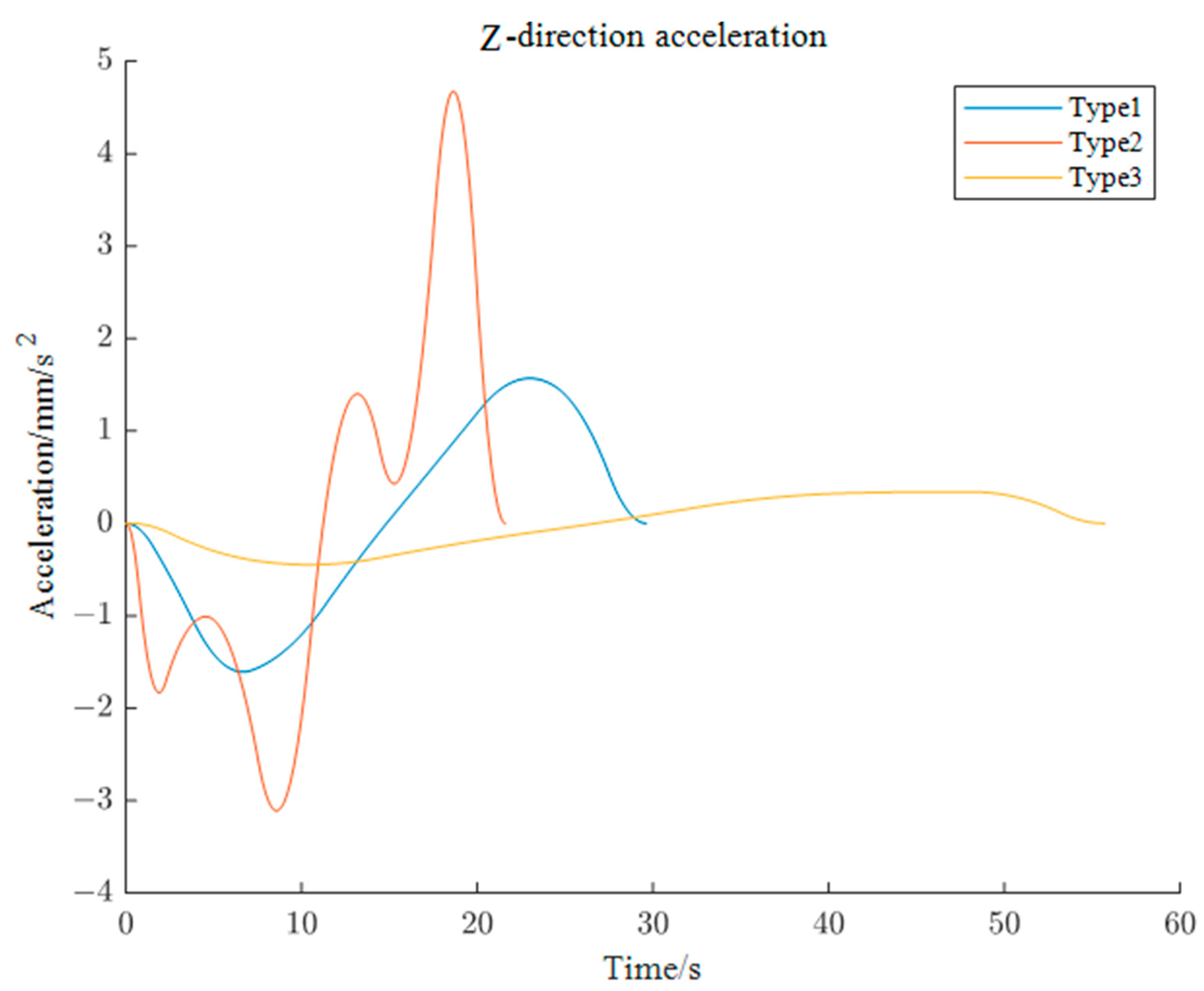
The Z-axis displacement, Z-axis velocity and Z-axis acceleration for the end of the left robotic arm are shown in Figure 19, Figure 20 and Figure 21, respectively. The displacement in the Z-axis direction is uniformly reduced from −1315 mm to −1515 mm. The Z-axis direction speed of Type 2 is relatively high, and a maximum value 18.19 mm/s is reaching but not exceeding 400 mm/s. The Z-axis acceleration of Type 2 is relatively high, and a maximum value 4.81 mm/s2 can be found but not more than 100 mm/s2.

6. Experimental Confirmation

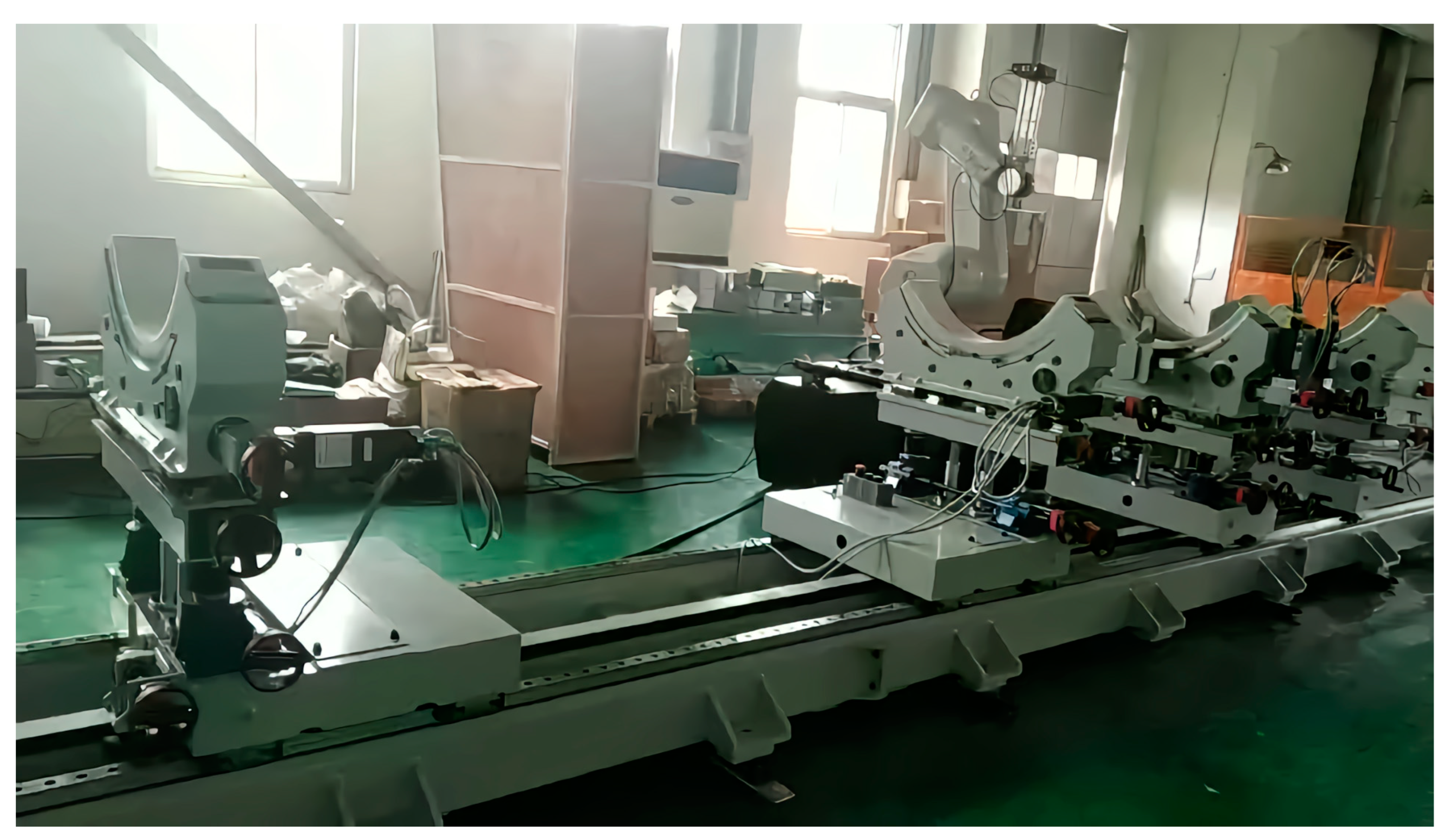
In order to verify the effectiveness of the algorithm, trajectory planning and tracking experiments of the cabin docking robot are conducted based on the cabin docking experimental platform. The cabin docking experimental platform is shown in Figure 22. One of the cabin-docking robots is selected as the research object for trajectory planning and trajectory following experiments.
In order to ensure the accuracy of the trajectory following control, explosion-proof servo motors are selected for driving the cabin docking experimental platforms. Based on the experimental platform, the trajectory generated by the modified multi-objective cuckoo algorithm is taken as the target trajectory, and the actual position is used as the target trajectory. Then, the experiments for the X-axis trajectory planning and the Z-axis trajectory planning are carried out.

6.1. X-axis Trajectory Planning

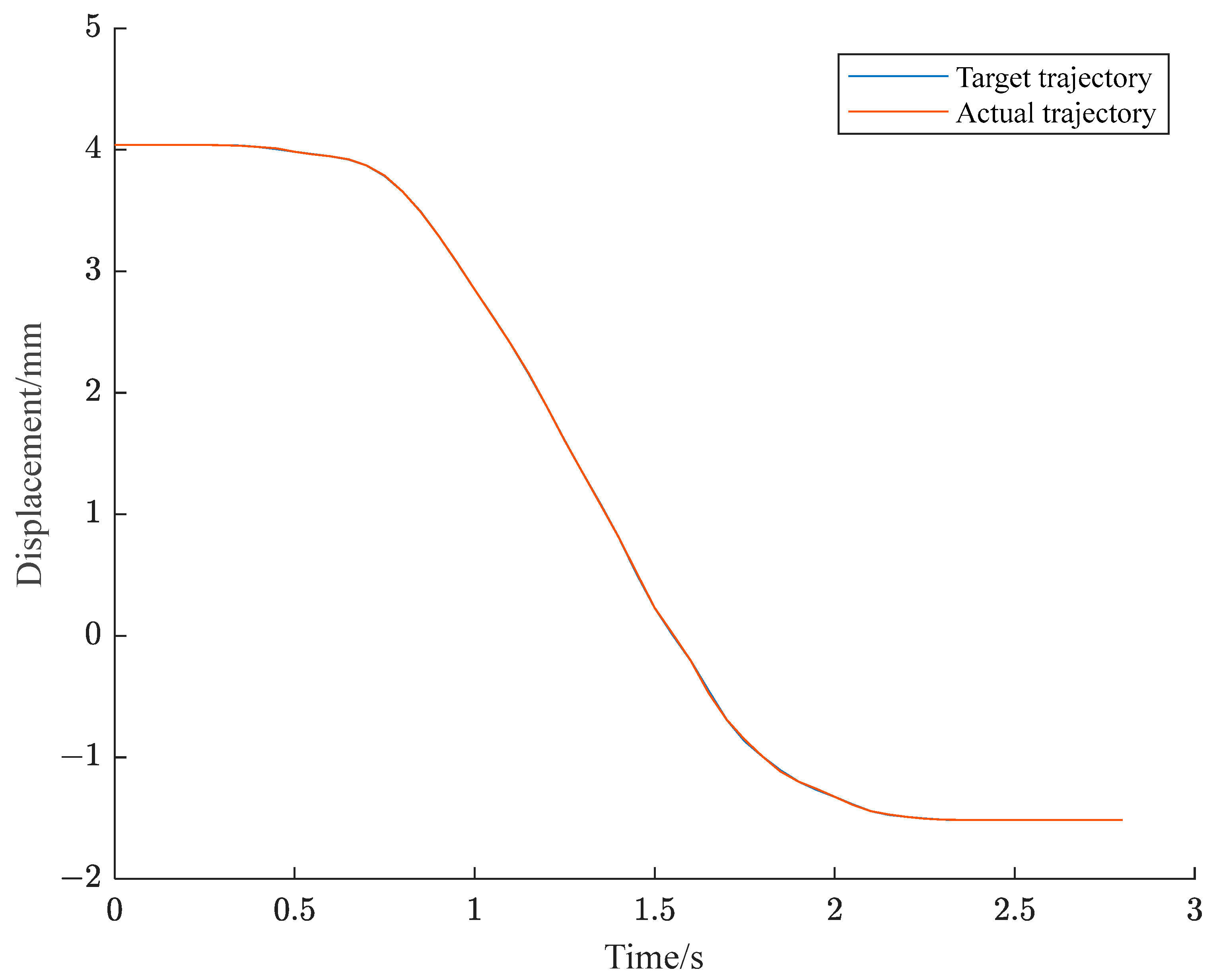
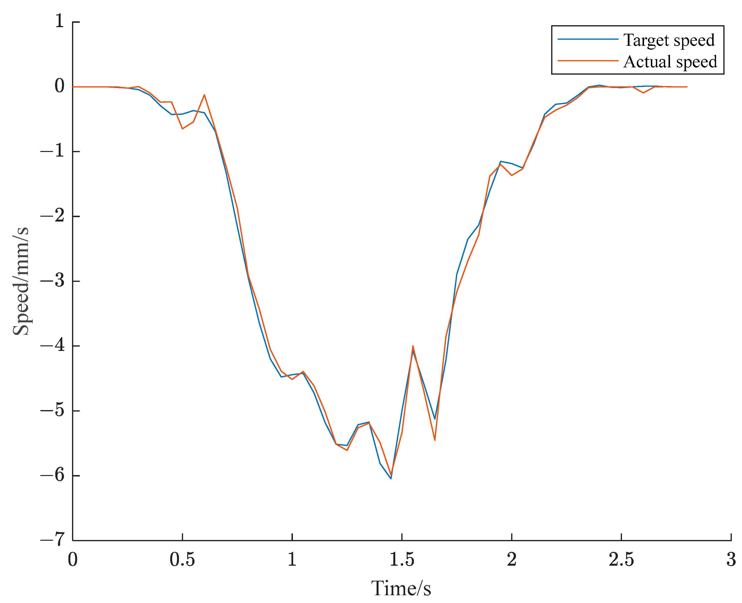
The starting position in the X-axis direction of the cabin docking robot is set as 4.04 mm, and the stopping position is −1.514 mm. The planned target trajectory is compared with the collected actual trajectory, which is given in Figure 23. A comparison between the planned target speed and the collected actual speed is shown in Figure 24. It is found that the maximum and minimum tracking errors of the X-axis trajectory are 0.014 mm and 0 mm, respectively. The maximum tracking error of the X-axis speed is 0.465 mm/s, and the minimum value is 0 mm. The error is very small.

6.2. Z-axis Trajectory Planning

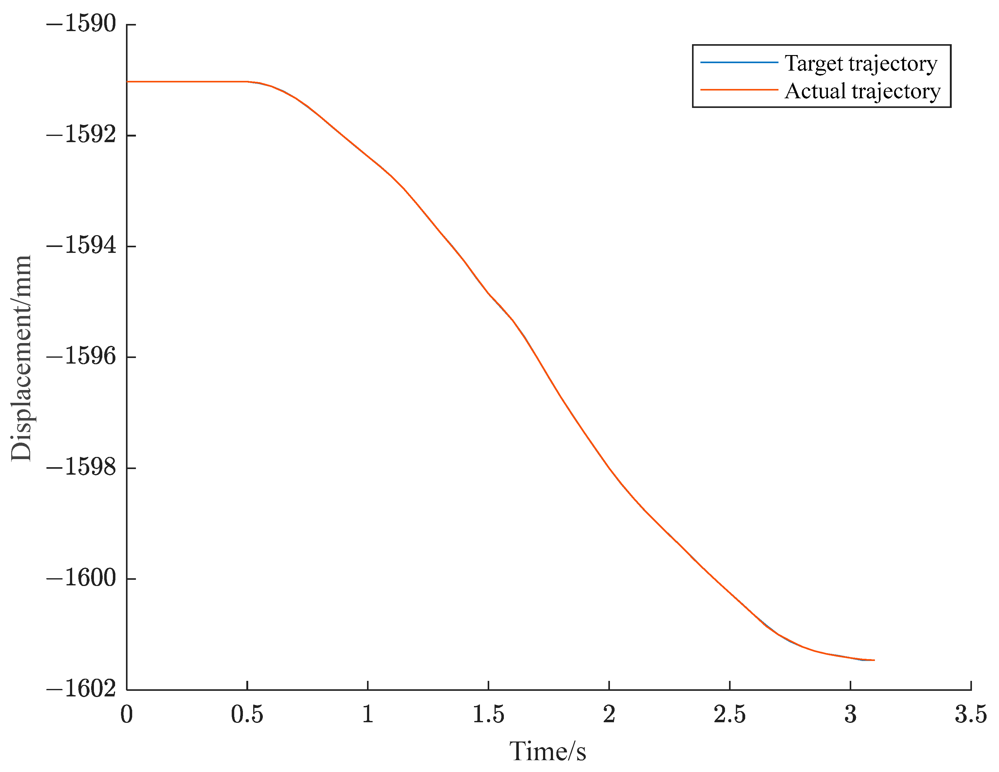
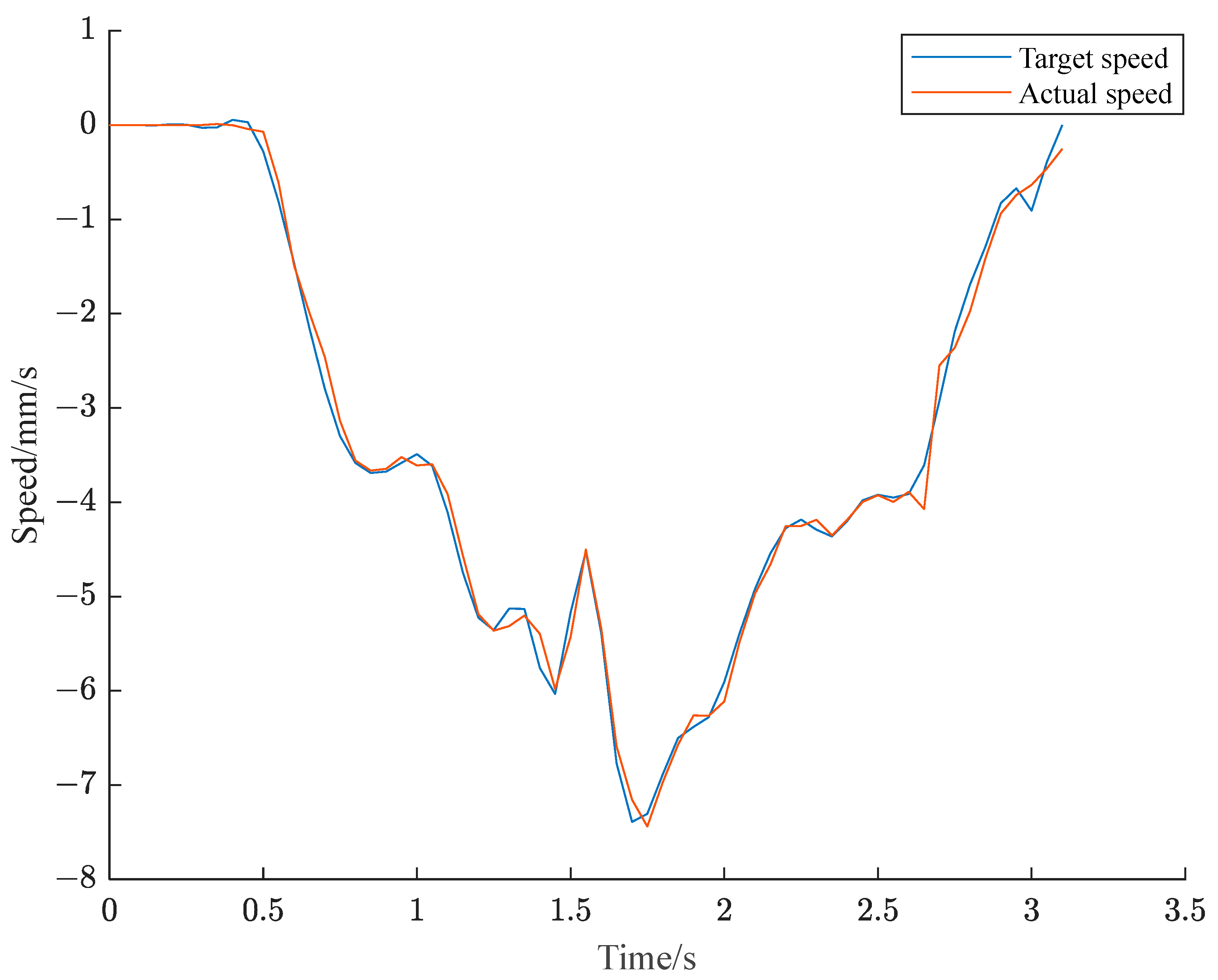
The starting position in the Z-axis direction of the cabin docking robot is set as −1591.03 mm, and the stopping position is −1601.47 mm. The comparison between the planned target trajectory and the collected actual trajectory is shown in Figure 25. The relative results for the speed can be seen in Figure 26. The maximum and minimum tracking errors of the Z-axis trajectory are 0.018 mm and 0 mm, respectively. The maximum tracking error of the speed is 0.364 mm/s, and the minimum value is 0 mm. The error is also very small, and the effectiveness of the modified cuckoo search algorithm is proven.

7. Conclusions

In order to ensure the accuracy and reliability of cabin docking, a multi-objective trajectory planning method for the dual-arm robot is proposed. The relative results are summarized as follows:
(1) A forward kinematics model of the cabin docking dual-arm robot is established based on the D-H modeling method, and the inverse kinematics analysis is also conducted. Based on the analysis of four different cabin attitudes, the relationship between the end trajectory and attitude parameters of the cabin-docking robot is studied. A trajectory planning scheme for the robotic arm is designed, and B-spline curve construction and parameterization methods are introduced.
(2) The selection method of objective function and comprehensive optimal solution is introduced. On the basis of the traditional multi-objective cuckoo algorithm, a modified multi-objective cuckoo search algorithm is proposed from two aspects: initial population generation method and cuckoo algorithm step size.
(3) The performance of the NSGA-II algorithm, MOPSO algorithm, MOCS algorithm and IMOCS algorithm are compared using simulations. Three types of normalization methods are selected: the optimal total time and joint target synthesis, the minimum total time and the minimum joint impact. The simulation analysis is conducted on the end effector of the cabin docking robot in the X-axis and Y-axis directions. The trajectory planning effect in the Z-axis direction is smooth in all three directions, and the maximum speed and acceleration in the X-axis direction are 2.39 mm/s and 1.39 mm/s2. The maximum operating speed in the Y-axis direction is 3.09 mm/s, and the maximum operating acceleration in the X-axis direction is 0.91 mm/s2. The maximum operating speed in the Z-axis direction is 18.19 mm/s, and the maximum operating acceleration in the Z-axis direction is 4.81 mm/s2. The simulation results can meet expectations, and the values are within the constraint range.
(4) On the basis of the cabin docking experimental platform, trajectory planning and tracking time of the end effector of the cabin docking robot in the X-axis and Z-axis directions are carried out. The maximum trajectory tracking error in the X-axis direction of the cabin docking robot is 0.014 mm, and the maximum velocity tracking error is 0.465 mm/s. The maximum trajectory tracking error in the Z-axis direction of the cabin docking robot is 0.018 mm, and the maximum velocity tracking error is 0.364 mm/s, which proves the effectiveness and feasibility of the modified algorithm.

Author Contributions

Conceptualization, R.L. and F.P.; methodology, R.L.; software, R.L.; validation, R.L.; formal analysis, R.L.; investigation, R.L.; resources, R.L.; data curation, R.L.; writing—original draft preparation, R.L.; writing—review and editing, F.P.; visualization, F.P.; supervision, F.P.; project administration, F.P.; funding acquisition, F.P. All authors have read and agreed to the published version of the manuscript.

Funding

We would like to express our gratitude to the National Natural Science Foundation of China (No.61973036) and the Science and Technology Cooperation Project of Yunnan Province (202003AD150002).

Data Availability Statement

Data are contained within the article and are available from the corresponding author on reasonable request.

Conflicts of Interest

There are no any personal circumstances or interest that may be perceived as inappropriately influencing the representation or interpretation of reported research results in this paper.

References

  1. Rüscher, O.; Mayländer, H. Automated alignment and marry-up of aircraft fuselage sections with a final assembly line. SAE Trans. 2001, 110, 173–178. [Google Scholar] [CrossRef]
  2. Bond, J. Mission critical: Precision in the air and on the ground. Mod. Mater. Handl. 2013, 68, 48–50. [Google Scholar]
  3. Kim, J.-J.; Lee, J.-J. Trajectory optimization with particle swarm optimization for manipulator motion planning. IEEE Trans. Ind. Inform. 2015, 11, 620–631. [Google Scholar] [CrossRef]
  4. Tian, L.; Collins, C. An effective robot trajectory planning method using a genetic algorithm. Mechatronics 2003, 14, 455–470. [Google Scholar] [CrossRef]
  5. Wang, H.; Wang, H.; Huang, J.; Zhao, B.; Quan, L. Smooth point-to-point trajectory planning for industrial robots with kinematical constraints based on high-order polynomial curve. Mech. Mach. Theory 2019, 139, 284–293. [Google Scholar] [CrossRef]
  6. Wang, S.; Wu, S.; Kang, C.; Li, X. Trajectory planning of a parallel manipulator based on kinematic transmission property. Intel. Serv. Robot. 2015, 8, 129–139. [Google Scholar] [CrossRef]
  7. Liu, L.; Chen, C.; Zhao, X.; Li, Y. Smooth trajectory planning for a parallel manipulator with joint friction and jerk constraints. Int. J. Control Autom. Syst. 2016, 14, 1022–1036. [Google Scholar] [CrossRef]
  8. Chen, Z.; Wang, J.; Li, S.; Ren, J.; Wang, Q.; Cheng, Q.; Li, W. An Optimized Trajectory Planning for Welding Robot. IOP Conf. Ser. Mater. Sci. Eng. 2018, 324, 012009. [Google Scholar] [CrossRef]
  9. Gasparetto, A.; Zanotto, V. A technique for time-jerk optimal planning of robot trajectories. Robot. Comput. Integr. Manuf. 2007, 24, 415–426. [Google Scholar] [CrossRef]
  10. Chen, D.; Li, S.; Wang, J.; Feng, Y.; Liu, Y. A multi-objective trajectory planning method based on the improved immune clonal selection algorithm. Robot. Comput. Integr. Manuf. 2019, 59, 431–442. [Google Scholar] [CrossRef]
  11. Lan, J.; Xie, Y.; Liu, G.; Cao, M. A Multi-Objective Trajectory Planning Method for Collaborative Robot. Electronics 2020, 9, 859. [Google Scholar] [CrossRef]
  12. Wang, Z.; Li, Y.; Shuai, K.; Zhu, W.; Chen, B.; Chen, K. Multi-objective Trajectory Planning Method based on the Improved Elitist Non-dominated Sorting Genetic Algorithm. Chin. J. Mech. Eng. 2022, 35, 81–95. [Google Scholar] [CrossRef]
  13. Wang, Y.-J.; Xing, K.; She, B.; Liu, Y.; Chen, T.; Hu, G.; Wu, Q. Mixed Gaussian stochastic inversion based on a hybrid of cuckoo algorithm and Markov chain Monte Carlo. Chin. J. Geophys. 2021, 64, 2540–2553. [Google Scholar] [CrossRef]
  14. Jiang, Y.; Shuai, L.; Wu, Q.; Cao, Y. Optimization of resonant parameters of bidirectional DC electronic transformer based on cuckoo algorithm. Acta Energiae Solaris Sin. 2021, 42, 485–494. [Google Scholar] [CrossRef]
  15. Huang, B.Y.; Zhang, Y.X.; Zhao, L. Research on Fault Diagnosis Method of Rolling Bearings Based on Cuckoo Search Algorithm and Maximum Second Order Cyclostationary Blind Deconvolution. J. Mech. Eng. 2021, 57, 99–107. [Google Scholar] [CrossRef]
  16. Lai, Y.W.; Zhang, J. Urban Bus Scheduling Optimization Based on Simulated Anneal-adaptive Cuckoo Search Algorithm. J. Transp. Syst. Eng. Inf. Technol. 2021, 21, 183–189. [Google Scholar] [CrossRef]
  17. Yang, X.S.; Deb, S. Multiobjective Cuckoo Search for Design Optimization; Elsevier Science Ltd.: Amsterdam, The Netherlands, 2013. [Google Scholar]
  18. Niknam, T.; Zare, M.; Gharibzadeh, M.; Azizipanah-Abarghooee, R. Multi-objective short-term scheduling of thermoelectric power systems using a novel multi-objective improved cuckoo optimization algorithm. Iet Gener. Transm. Distrib. 2014, 13, 1546–1550. [Google Scholar] [CrossRef]
  19. Wang, H.; Sheng, B.; Lu, Q.; Luo, R.; Fu, G. A Multi-Objective Cuckoo Search Algorithm Based on the Record Matrix for a Mixed-Model Assembly Line Car-Sequencing Problem. IEEE Access 2020, 8, 76453–76470. [Google Scholar] [CrossRef]
  20. Singh, G.; Banga, V.K. Kinematics and trajectory planning analysis based on hybrid optimization algorithms for an industrial robotic manipulators. Soft Comput. 2022, 26, 11339–11372. [Google Scholar] [CrossRef]
  21. De Boor, C. On Calculation with B-spline. J. Approx. Theory 1972, 6, 50–62. [Google Scholar] [CrossRef]
  22. Cox, M.G. The numerical evaluation of B-spline. J. Inst. Maths. Appl. 1972, 10, 134–149. [Google Scholar] [CrossRef]
  23. Kahagalage, S.; Turan, H.H.; Jalalvand, F.; El Sawah, S. A novel graph-theoretical clustering approach to find a reduced set with extreme solutions of Pareto optimal solutions for multi-objective optimization problems. J. Glob. Optim. 2023, 86, 467–494. [Google Scholar] [CrossRef]
  24. Zhang, X.S.; Liu, J.; Luo, S.B. An improved multi-objective cuckoo search algorithm for airfoil aerodynamic optimization design. Acta Aeronaut. Astronaut. Sin. 2019, 40, 122500. (In Chinese) [Google Scholar] [CrossRef]
  25. Wang, L.P.; Ren, Y.; Qiu, Q.C.; Qiu, F.Y. Survey on Performance Indicators for Multi-objective Evolutionary Algorithms. Chin. J. Comput. 2021, 44, 1590–1619. (In Chinese) [Google Scholar] [CrossRef]
  26. Van Veldhuizen, D.A.; Lamont, G.B. On measuring multi-objective evolutionary algorithm performance. In Proceedings of the 2000 Congress on Evolutionary Comutation, La Jolla, CA, USA, 16–19 July 2000; Volume 204, p. 211. [Google Scholar]
  27. Van Veldhuizen, D.A. Lamont G B. Evolutionary computation and convergence to a Pareto front. In Proceeding of the Late-breaking Paper at the Genetic Programming 1998 Conference, Madison, WI, USA, 22–25 July 1998; pp. 221–228. [Google Scholar]
  28. Schoxtt, J.R. Fault-Tolerant Design Using Single and Multicriteria Genetic Algorithm Optimization. Master’s Thesis, Air Force Institute of Technology, Wright-Patterson AFB, OH, USA, 1995. [Google Scholar]
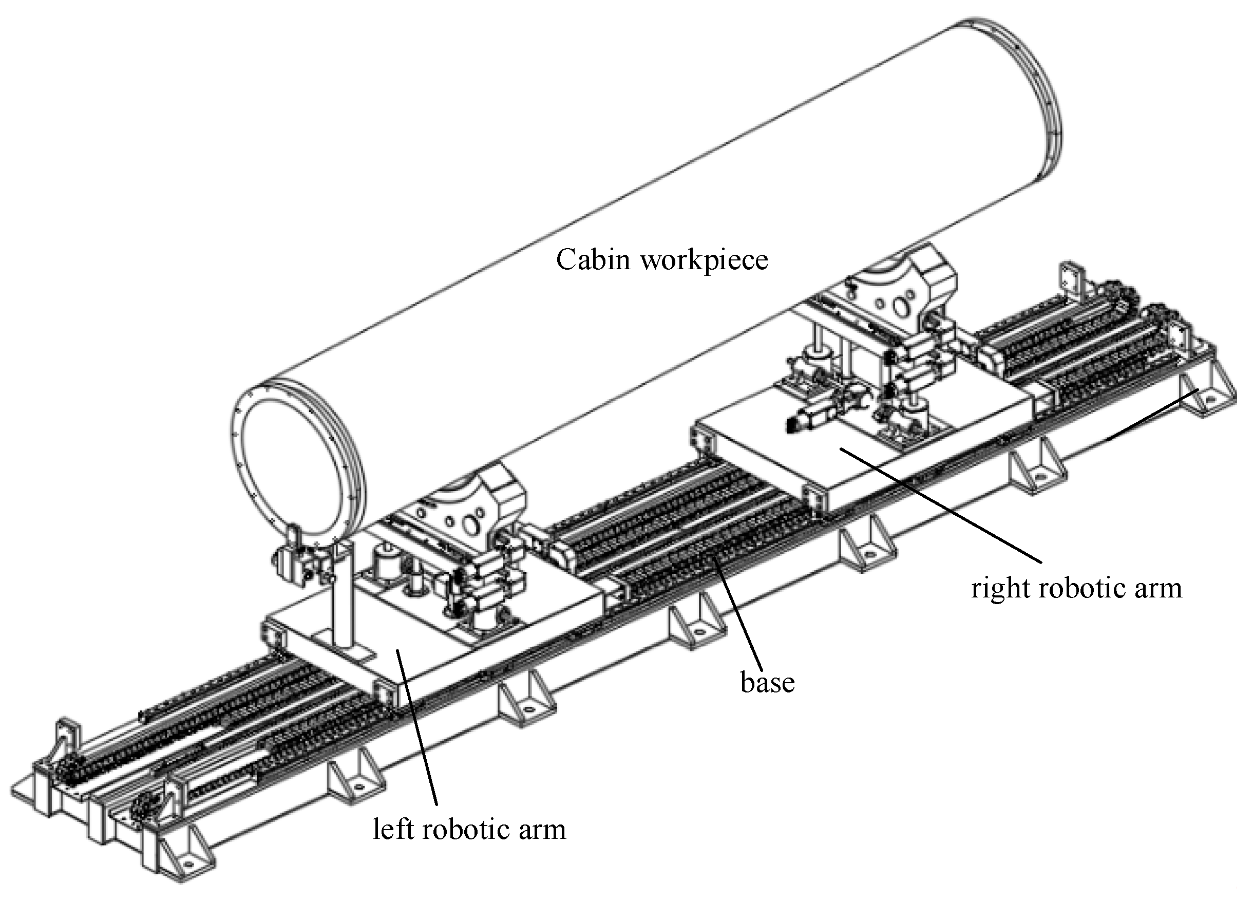
Figure 1. The cabin docking dual-arm robot.
Machines 12 00064 g001
Figure 2. Components of the right robotic arm.
Machines 12 00064 g002
Figure 3. The simplified model and joint coordinate systems of the cabin docking dual-arm robot.
Machines 12 00064 g003
Figure 4. Distribution of coordinate systems for dual-arm robot docking in cabin section.
Machines 12 00064 g004
Figure 5. The attitude parameters of the cabin section workpiece.
Machines 12 00064 g005
Figure 6. Coordinate system situation of the initial balance position.
Machines 12 00064 g006
Figure 7. Coordinate system situation when the pitch angle is not at 0°.
Machines 12 00064 g007
Figure 8. Coordinate system situation when the yaw angle is not at 0°.
Machines 12 00064 g008
Figure 9. Coordinate system situation when roll angle γ is not at 0°.
Machines 12 00064 g009
Figure 10. Calculation process of trajectory planning for 5th degree B-spline curves.
Machines 12 00064 g010
Figure 11. Flow chart of the trajectory optimization.
Machines 12 00064 g011
Figure 12. Pareto frontier for robot arm trajectory planning.
Machines 12 00064 g012
Figure 13. Left robotic arm X-axis displacement curve.
Machines 12 00064 g013
Figure 14. Left robotic arm X-axis speed curve.
Machines 12 00064 g014
Figure 15. Left robotic arm X-axis acceleration curve.
Machines 12 00064 g015
Figure 16. Left robotic arm Y-axis displacement curve.
Machines 12 00064 g016
Figure 17. Left robotic arm Y-axis speed curve.
Machines 12 00064 g017
Figure 18. Left robotic arm Y-axis acceleration curve.
Machines 12 00064 g018
Figure 19. Left robotic arm Z-axis displacement curve.
Machines 12 00064 g019
Figure 20. Left robotic arm Z-axis speed curve.
Machines 12 00064 g020
Figure 21. Left robotic arm Z-axis acceleration curve.
Machines 12 00064 g021
Figure 22. Docking experiment platform.
Machines 12 00064 g022
Figure 23. X-axis trajectory planning curve of cabin docking robot.
Machines 12 00064 g023
Figure 24. Speed planning curve in the X-axis direction for the docking robot.
Machines 12 00064 g024
Figure 25. Z-axis trajectory planning curve of cabin docking robot.
Machines 12 00064 g025
Figure 26. Speed planning curve in the Z-axis direction for the docking robot.
Machines 12 00064 g026
Table 1. D-H parameters for the cabin docking dual-arm robot.
LinkJoint Angle θiLink Offset diLink Length aiLink Angle αi
Base-L0π/200−π/2
L10dL10π/2
L2−π/2dL20π/2
L3π/2dL3dLπ/2
L4θLdL400
Base-R0π/200π/2
R10dR10−π/2
R2π/2dR20−π/2
R3−π/2dR3dR−π/2
R4θRdR400
Table 2. Design parameters of cabin docking robot.
NumberParameterValue
1Roll angle range±15°
2Z-axis direction travel range±600 mm
3Y-axis direction travel range±50 mm
4X-axis direction travel range±50 mm
5Roll angle speed range0~6.8°/s
6Z-axis direction speed range0~400 mm/s
7Y-axis direction speed range0~25 mm/s
8X-axis direction speed range0~2.5 mm/s
9Roll angle acceleration range0~240°/s2
10Z-axis direction acceleration range0~100 mm/s2
11Y-axis direction acceleration range0~100 mm/s2
12X-axis direction acceleration range0~100 mm/s2
Table 3. The 11 sets of IMOCS trajectory planning non-dominated solutions.
Serial NumberTotal TimeJoint Impact
121.57433.9448
223.40571.5797
324.72171.0077
427.58310.6339
531.98160.3965
634.39130.3104
738.19780.2363
842.67960.1724
944.92170.1483
1051.12230.1025
1159.56780.0753
Table 4. Normalized weight coefficient setting table.
Typew1w2
111
201
310
Disclaimer/Publisher’s Note: The statements, opinions and data contained in all publications are solely those of the individual author(s) and contributor(s) and not of MDPI and/or the editor(s). MDPI and/or the editor(s) disclaim responsibility for any injury to people or property resulting from any ideas, methods, instructions or products referred to in the content.