1. Introduction
Predicting operation conditions and prognostic remaining life in machinery has been researched for decades. Nevertheless, several operating conditions modify predictions and require different processing techniques. The most relevant prognostic methods are based on the analysis of vibrations signals. These methods have evolved based on sensor technologies, signal processing techniques, and data analytics advances. The methods base their predictions on relating the vibration characteristics identifying the excitation frequencies of every mechanical component and evaluating the evolution of every signal’s amplitude [
1].
Prognostic methods have evolved from simple diagnostic techniques to artificial intelligence methods. The simple diagnosis techniques focus on frequency spectrum analysis using the fast Fourier transform, the time-domain analysis of the signal waveform, and the statistical variations in the vibration response. The first method evaluated the RMS (root mean square value) changes of the entire signal. The big disadvantage of this method is that high-frequency signal components hardly modify the RMS value, and most of the early failures occur in mechanical elements that excite higher frequencies. The RMS evaluation is useful for machines that produce vibrations at a single frequency (like heavy rotors with a dominant frequency around the rotating speed).
The advances in signal analysis open the opportunity to transform vibration signals into frequency spectrums (these techniques are based on the convolution theorem and numerical methods such as the fast Fourier transform). In this way, relevant features were identified in the frequency spectrum. Besides FFT, other signal processing methods, such as wavelet transform (continuous and discrete) and empirical mode decomposition (EMD), are applied to improve feature identification. The statistical moments were also applied to extract significant information from raw vibration data and to estimate time-to-failure scenarios.
Identification methods were complemented with model-based approaches. These approaches utilize physical models to describe the machine’s dynamic behavior and simulate vibration responses under different operating conditions and fault scenarios. By comparing numerical predictions with field measurements, it is possible to identify faulty conditions, predict the remaining life, and estimate the time-to-failure.
Recent developments are based on artificial intelligence (AI) techniques [
2,
3]. Once failure conditions are preprocessed, data can be clustered, and prognostics can be achieved using either machine learning, neural networks [
4], data-driven techniques, decision trees, or random forest algorithms. Artificial neural networks consist of layers of interconnected nodes that process information recorded from the vibration signal; then, they are trained to identify and predict the occurrence of failures. Convolutional neural networks (CNNs) are deep learning algorithms commonly used in image and signal processing tasks [
4]. Decision trees use a tree-like structure to characterize the failure nature and set scenarios of possible consequences. Decision trees can be trained using historical data to predict the occurrence and severity of faults based on vibration data. SVMs are a type of machine learning algorithm that is commonly used in classification tasks. They work by finding the optimal hyperplane that separates different classes in the data. They use historical data to predict the occurrence and severity of faults based on vibration data [
3,
5,
6].
Correlating multiple signal sensors enhance the accuracy and reliability of the prognostic methods. Vibration signals can be correlated to temperature measurements, power consumption, torque, and other signals, such as acoustic emissions. Based on the correlation of different signals, it is possible to eliminate fictitious faults, and it is complemented with production signals obtained from PLC controllers and SCADA systems [
7].
Big data analytics has helped analyze a large amount of data [
8]. The use of large amounts of generated and stored data in complex manufacturing plants, farms with large numbers of wind turbines, or assembly lines cannot be analyzed without big data analytics. The identification of faults is possible when the vibration data are analyzed in real-time, and these techniques have proven to handle vast amounts of data and provide accurate predictions of impending failures. Civera and Surace [
9] applied instantaneous spectral entropy to predict the operating conditions of wind turbines. They combined spectral entropy and continuous wavelet transform to determine the machine conditions and generate the data for a CMS.
Recent works have sought other tools to extract machine features, mainly when non-stationary and nonlinear responses modify vibration signals [
10,
11]. Recurrence plots (RP) have proven to be a powerful tool for CMSs, particularly for detecting faults in wind turbines under gusty winds. RPs provide a visual and quantitative representation of the system dynamics that can help identify problems before they become more severe or result in downtime or costly repairs. If the machinery operates in normal conditions, the RP will have a regular pattern, indicating that the system’s dynamics are stable. However, if there is a fault or damage to the machinery, the RP will typically exhibit changes in its pattern, such as the appearance of new diagonal lines or the disappearance of existing ones [
12].
ARIMA is a method that has been applied to different research fields and has shown excellent results [
13]. In a condition monitoring system, the ARIMA model determines the baseline pattern of healthy machine elements and sets the reference value for each characteristic frequency. It can extrapolate the tendencies and can predict possible time-to-failure scenarios. Predictions are updated with current measurements. For better results, the data window is updated at smaller intervals every time there is a significant amplitude increment. Since condition monitoring systems are based on the analysis of measurements recorded at even intervals, the data are treated as time series models. This treatment allows forecasting the operating conditions with ARIMA and can be applied to different systems, regardless of their physical behavior. Zhou et al. [
14] combined ARIMA and the generalized auto-regressive conditional heteroscedasticity (GARCH) models to predict wireless network traffic. Farhan Mohammad Khan and Rajiv Gupta used ARIMA to compare the accuracy of the expected model with a nonlinear autoregressive (NAR) neural network in a similar situation [
15]. Artificial intelligence-based regression models are a solution for creating models that predict or forecast the future values of time series measurements. AI-based algorithms are frequently used for complex data models. This regression approach automatically detects correlations between input and output variables. Thus, the ARIMA method forecasts Internet traffic, resource allocation, and network anomaly detection caused by attacks [
16].
ARIMA has also been used to determine Internet traffic’s short and long dependencies. Although its predictions are less accurate than other methods, its simplicity and traceability to the data source make it a good alternative for forecasting time series with random variations [
17].
Different faults can be identified by analyzing the time-frequency characteristics, such as unbalance, misalignment, bearing and gear defects, rubbing, or loose elements. These failures have characteristic frequencies that should not be present or have very low amplitudes when the machine is new and healthy. When they appear, the spectrum will show a significant change in the amplitude value, and the ARIMA algorithm will detect the change. The same situation occurs when any anomalous event happens. The ARIMA algorithm will trigger alarm conditions when it detects a sudden change in the vibration signal. Every component produces vibration signals whose frequencies are proportional to the rotating speed. But in the case of wind turbines, the rotating speed is not constant. It depends on the wind velocity. Thus, the ARIMA algorithm requires that the vibration signal be indexed to the rotating speed. ARIMA models can provide insights into the expected vibration behavior over time by analyzing long-term trends and patterns. It is worth noting that while ARIMA models can capture the temporal dependencies and trends in vibration signals, more advanced techniques, such as autoregressive integrated moving average with exogenous inputs (ARIMAX) or machine learning algorithms, may be employed to incorporate additional factors like temperature, operating conditions, or load variations for more accurate predictions and analysis.
Several works discuss the application of ARIMA to vibration data. Al-Bugharbee et al. [
18], Gao et al. [
19], and Luo et al. [
20] explored the application of time series analysis techniques, including ARIMA models, for vibration data analysis in condition monitoring. These papers discuss the process of modeling vibration signals using ARIMA models and demonstrate the approach’s effectiveness in detecting faults and predicting future vibration levels. Sun et al. [
21], Ganga and Ramachandran [
22], and Yang et al. [
23] focused on predicting the vibration signals of rotating machinery using ARIMA models. It presents a detailed methodology for modeling and forecasting vibration signals based on historical data. The paper also discusses the application of ARIMA models in fault diagnosis and condition monitoring. These researchers investigated the application of ARIMA models for the fault diagnosis of rolling bearings based on vibration signals. They presented a methodology for feature extraction from vibration data and demonstrated using ARIMA models to identify different types of bearing faults. The study highlighted the effectiveness of ARIMA models in diagnosing faults and discussed the approach’s advantages.
The evolution of prognostic methods based on vibration signals has transitioned from simple diagnostic expert systems to sophisticated data-driven approaches that can handle vast amounts of data in short periods. The accuracy and speed of modern sensors, plus the practical design of big data algorithms, have improved the identification of failures and the prognostics of the remaining useful life of machines and structures. Mahajan et al. modeled wireless traffic networks with six algorithms: decision “tree regressor”, “linear regression”, “multi-layer perceptron”, “Poisson regression”, “ARIMA, and “LSTM”. The system was evaluated at different intervals, and the “LSTM” algorithm was the best-performing [
6]. Their data showed variations less significant than those produced by gusty winds.
This paper presents the application of the auto-regressive integrated moving average (ARIMA) algorithm to predict failures in wind turbines. This method was selected because it forecasts vibration signals measured on machinery under loading conditions that change suddenly, such as the case of wind turbines operating under gusty winds. In contrast with exponential forecasting, ARIMA has shown effective results in fields such as finance, economics, and weather forecasting by predicting future conditions based on historical patterns and trends. It also has shown promising results in predicting faults in rotating machinery (pumps, turbines, electric motors, bearings, and gearboxes) and estimating time-to-failure dates for scheduling maintenance works before catastrophic breakdowns.
2. Auto Regressive Integrated Moving Average (ARIMA) Algorithm
Although the auto-regressive integrated moving average (ARIMA) algorithm has been used for some time, it is a time series forecasting method that predicts future values based on historical data. It is very effective for predicting failures when the operating conditions are unsteady and have sudden changes, like in wind turbines. Whereas exponential forecasting is well suited for steady-state conditions, this method adjusts an exponential function to the historical vibration data. The data is recorded at time intervals that depend on a maintenance program and predict, based on the statistical evolution of the data, the time-to-failure date. But the exponential forecasting predictions have no sensitivity to sudden and short-term changes.
ARIMA combines an auto regression (AR) component, a differencing (D) component, and moving average (MA) component. The autoregressive component estimates the output variable as a linear combination of its historical values, similar to linear regression. The order of the autoregressive terms (p) determines the number of lagged observations used for prediction. The ARIMA method includes a differentiating component (D) to remove the trend in the vibration data. It takes the backward difference of consecutive observations and smooths the series, eliminating non-stationary terms. The differencing parameter specifies the differentiating order. The other characteristic component is the moving average; this component represents the dependency between error terms and residual errors from previous data. It estimates random fluctuations and noise. The number of moving average terms affects the predictions and is set with the (q) parameter.
The ARIMA model is written as ARIMA (p, D, q), where:
- -
p: the order of the autoregressive component, indicating the number of lagged observations.
- -
D: the order of differencing, indicating the number of times differencing is applied.
- -
q: the order of the moving average component, indicating the number of lagged forecast errors.
The ARIMA algorithm analyzes the time series data to identify trends or seasonality. If the series is non-stationary, apply the differencing component to make it stationary, but in the case of sudden changes, selecting this parameter is fundamental for obtaining good predictions. The next step is determining the order of differencing (D) by observing how many differencing steps are required to achieve stationarity. Then, the final step is to analyze the autocorrelation and partial autocorrelation plots to determine the order of autoregressive terms (p) and moving average terms (q). It is essential to differentiate data by estimating the model parameters using methods like maximum likelihood estimation to fit the ARIMA model for predicting future values. Once the model is fitted, it can predict future time points.
Vibration data have terms based on auto-regression, and some are based on moving averages. If terms in the time series have slight differences, then increase the autocorrelation terms (p), and if it has many differences, then the algorithm includes more moving average terms. If the data has a significant tendency, then d must be included; otherwise, it must be set to 1. In the case of vibration signals, the trend is minimal when there are no defects. But, in the case of sudden amplitude changes, p and q are critical in providing the most appropriate forecasting model. Plotting the correlation between predictions and original data versus p and q allows the identification of the best parameters. The (p, q) for the best model is performed based on the spikes and curve in the graph. The evaluation of the forecasting involves the use of other statistical analyses such as the Akaike information criterion (AIC), Bayesian criterion (BIC), and mean square error measurement [
24]. In this paper, the validation of the model is evaluated using the maximum likelihood estimation that determines the model’s accuracy to the historical data. The residual analysis and the goodness-of-fit test determines the model’s performance and the forecast errors. In this case, the q and p values are selected based on determining the minimum variance in the predictions. In some cases, the data is normalized, then the predicted values must be transformed back to the original scale to have correct units.
Once the model is fitted and validated, it can predict future time points. These predictions can provide insights into the expected vibration behavior and aid in maintenance planning or fault detection. It’s important to note that ARIMA models have limitations when dealing with complex or highly nonlinear vibration signals. More advanced modeling techniques like machine learning algorithms or nonlinear time series models may be more suitable in such cases. Nevertheless, predictions are well-fitted for wind turbines operating under gusty winds, and ARIMA is more straightforward than other AI algorithms. For this reason, ARIMA is suited for applications when short-term responses are needed.
The following is the description of the ARIMA algorithm:
- 1.
The first step is to calculate the autoregressive component. It sets the linear relationship between the vibration signal; in the case presented in this paper, it is one of the bearings frequencies of the gearbox. The future value is estimated as a weighted sum of previous values or lagged observations. The parameter p determines the number of lagged observations used for the prediction. As a difference from other methods, this parameter can be modified depending on the variability of the input data. This component is represented as AR(p).
Mathematically, the AR(p) component is defined as:
where:
- -
represents the amplitude of the vibration component at the bearing frequency (it can be any component of the vibration signal);
- -
is a constant term;
- -
are the autoregressive coefficients;
- -
is the error term or residual at time t.
- 2.
The differencing component removes trends or seasonality in the data and makes it stationary. Stationarity implies that the statistical properties of the data, such as mean and variance, do not change over time. Differencing involves subtracting the current observation from a previous observation, usually with a lag of one time. The “d” parameter in ARIMA represents the differencing order and determines how often differencing is applied to achieve stationarity. In the case of wind turbines, this parameter is set to one; in this way, sudden changes are easily predicted.
Mathematically, the differencing component can be represented as:
where
denotes the differenced series at time
t.- 3.
The moving average component captures the relationship between the variable and past forecast errors or residuals. It models the random fluctuations or noise in the data. The “q” parameter in ARIMA represents the order of the moving average terms and determines the number of lagged forecast errors used for prediction. The MA component can be represented as MA (q).
Mathematically, the MA(q) component is defined as:
where
denotes the residual at time
t, and
,
…,
are the moving average coefficients.
Combining these components, the ARIMA model can be represented as ARIMA (p, d, q). The model is constructed as follows:
The ARIMA algorithm involves the following steps:
- 1.
Analyze the time series data and determine if it requires differencing to achieve stationarity.
- 2.
Identify the orders (p, D, q) of the ARIMA model based on autocorrelation and partial autocorrelation plots.
- 3.
Estimate the model parameters (, , , …, ) using methods like maximum likelihood estimation.
- 4.
Validate the model by examining the residuals, conducting goodness-of-fit tests, and assessing forecast accuracy.
- 5.
Use the fitted ARIMA model to make predictions for future time points.
ARIMA models provide a robust framework for time series forecasting, but their effectiveness depends on the quality and characteristics of the data, the appropriate selection of model parameters, and the underlying assumptions being met. ARIMA models are commonly used for analyzing and forecasting stationary time series data. However, additional steps are required to make the data stationary before applying ARIMA when dealing with non-stationary vibration signals. Non-stationary vibration signals exhibit trends, seasonality, or other systematic patterns over time, which violate the assumptions of ARIMA models. The following approach can be followed for applying ARIMA to non-stationary vibration signals:
Visualize and analyze the data: Begin by visualizing the vibration signal and inspecting it for any apparent trends, seasonality, or other patterns. Visualization can be performed through time series plots, autocorrelation plots, or spectral analysis.
Detrending: If a clear trend is observed in the data, detrending can be performed to remove it. Detrending can be achieved by applying mathematical techniques such as differencing or polynomial fitting. Differencing involves taking the difference between consecutive observations, while polynomial fitting involves fitting a curve to the data and subtracting it to obtain residuals. In the case of recording the vibration amplitude at a specific frequency, data should not have any trend since the trend is related to premature failures or part degradation.
Seasonal adjustment: If seasonality is present in the data (e.g., repeating patterns occurring at fixed intervals), it needs to be addressed. Seasonal adjustment methods like seasonal differencing or seasonal decomposition of time series can be applied to remove the seasonal component. Regarding vibration data, seasonality can be related to different operating conditions or the dependency on sizeable periodic load changes.
Stationarity check: After detrending and seasonal adjustment, verifying if the data has become stationary is essential. Stationarity implies that the statistical properties of the data, such as mean and variance, remain constant over time. Stationarity can be assessed using statistical tests like the Augmented Dickey–Fuller or Kwiatkowski–Phillips–Schmidt–Shin test.
3. Results
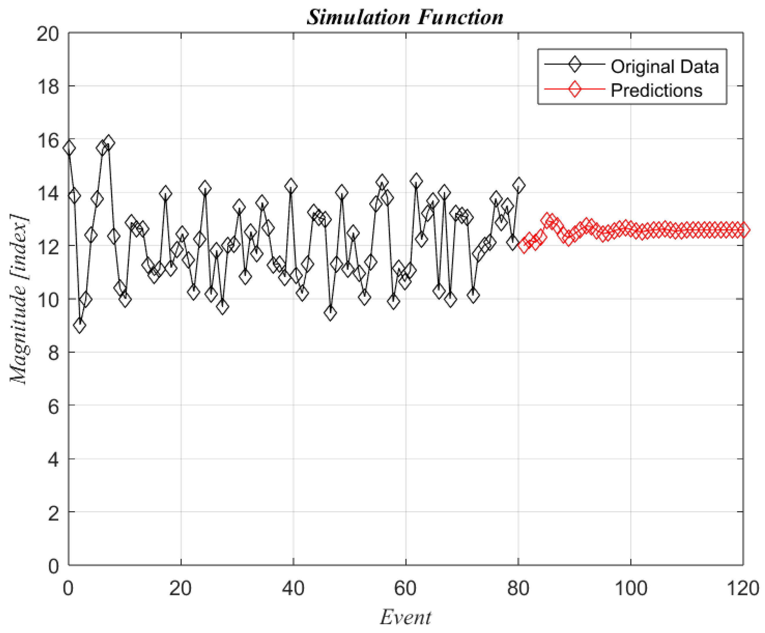
Data produced with a simulation function was tested to evaluate the method’s ability. The function was a simple sinusoidal with a logarithmic decrement. For forecasting new data, the model was tested with 50% more time values. The simulation function was:
where
represents white noise.
Several solutions were analyzed, including different levels of noise. The noise level amplitudes tested were 0, 1, and 5. The analysis included variations in the noise level and prediction with varying values of p and q.
Figure 1 shows the results of the original function without noise and p = 1 and q = 1.
Figure 2 presents the analysis with the same p and q values but with a noise amplitude of 1, and
Figure 3 is similar but with a noise amplitude of 5.
It is clear that the noise level affects the predictions, and it is essential to include higher values of q. The moving average terms give better predictions for unsteady signals from this simple function. The following figures (
Figure 4 and
Figure 5) show the results of the predictions with high noise levels (amplitude equal to 5) and two q values.
Predictions with a higher value for the autoregressive and moving average terms produce better results since it considers the original signal fluctuations and the unsteady noise values. This characteristic is the feature of the ARIMA algorithm that makes it suitable for predicting wind turbines’ operating conditions, mainly when gusty winds are present.
After analyzing the effect of the (p, D, q) parameters on simulated data, the algorithm was used to analyze vibration data. The ARIMA algorithm was used to predict the dynamic behavior of a 12 m wind turbine that operates under gusty winds. The vibration data was recorded at regular intervals during 80 events; the raw data were analyzed with the Fourier transform and the continuous wavelet transform to identify the dominant peaks. The wind turbine consists of a two blades rotor, a central shaft, a gearbox, and a permanent magnet generator. For the present work, only the dominant frequency of one gearbox bearing was analyzed. Only the amplitude variations at this frequency were used as the input data for this analysis. The frequency spectrums were normalized to adequate the values for the speed changes.
3.1. Experimental Description
Figure 6 shows a sketch and a picture of the experimental wind turbine installed at the Autonomous University of Queretaro. The wind turbine consists of a rotor, a main shaft, a speed increaser, and a permanent magnet 12 kW electric generator. The increaser (gearbox with a 1:2.01 speed ratio) was instrumented with a three-axes MEMs accelerometer, three orthogonal gyroscopes, and a temperature sensor (ADX321J Analog Devices
®, Wilmington, MA, USA) The acceleration data was recorded at even events, and the data was analyzed with a continuous wavelet spectrogram, and the highest amplitudes around the bearing frequency were used to forecast the gearbox bearing condition.
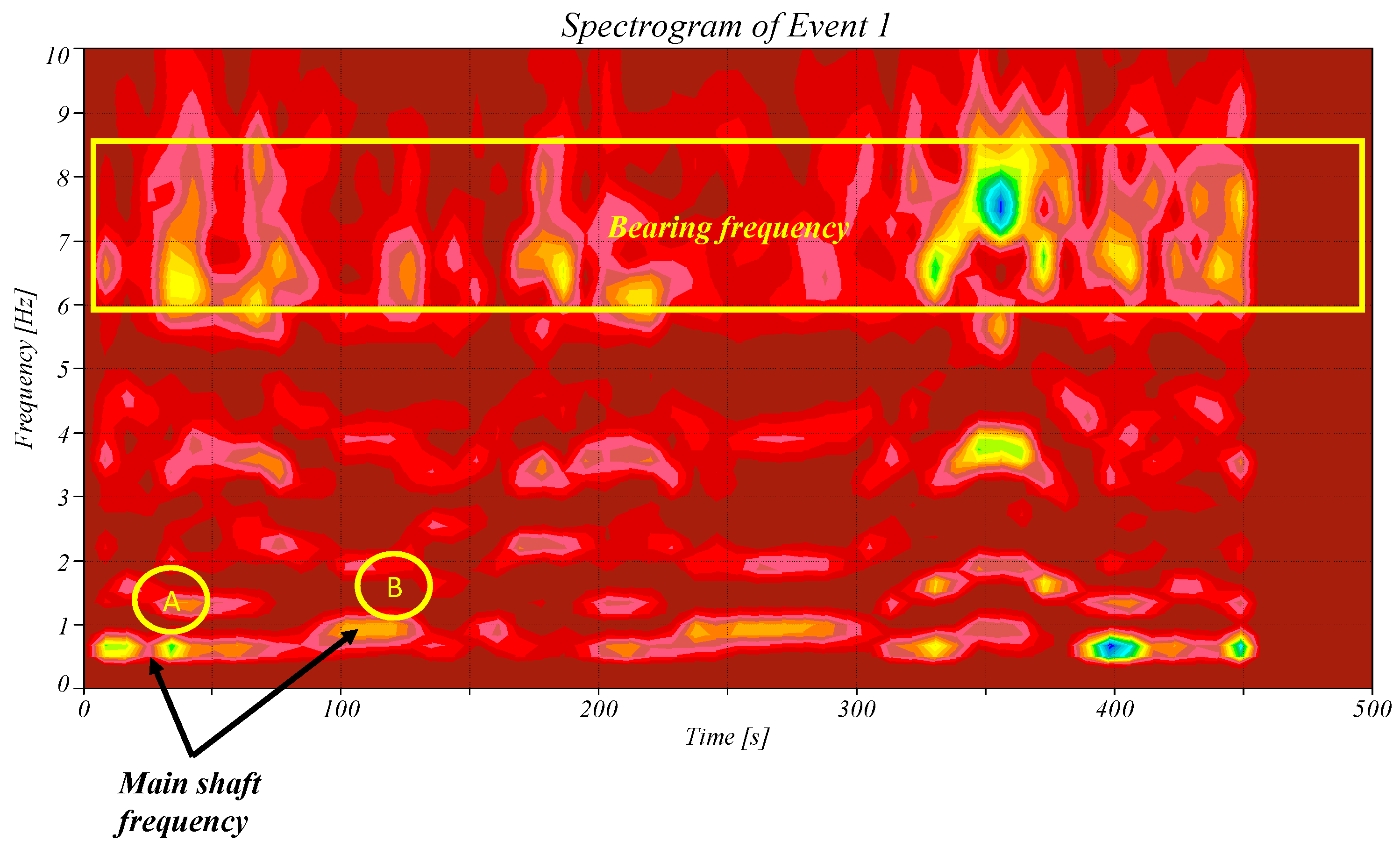
Figure 7 shows the spectrogram of event one. The main shaft frequency is marked with points A and B. This figure shows the speed variations (different frequencies between points A and B). The highest peaks at the bearing frequency are also highlighted. This figure also shows the highest amplitude that was recorded at event 1. The spectrogram shows the highest amplitudes at 350 s and 400 s. This difference indicates that the wind turbine has highly nonlinear responses, and the gusty wind affects each component differently. High amplitudes at the bearing frequency occur before the highest peaks at the main rotor’s frequency.
3.2. Experimental Results
Figure 8 shows the amplitude values of the dominant frequency of the gearbox bearings. The amplitude increased up to five times the steady conditions. These values were the result of sudden events related to gusty winds. When the wind blows steadily, the vibration amplitude oscillates between 0.01 to 0.04; thus, it can be noticed that the gusty winds occurred at random intervals.
3.3. Calibration of the ARIMA Parameters
P and q parameters are determined based on evaluating the likelihood between the original data and predictions [
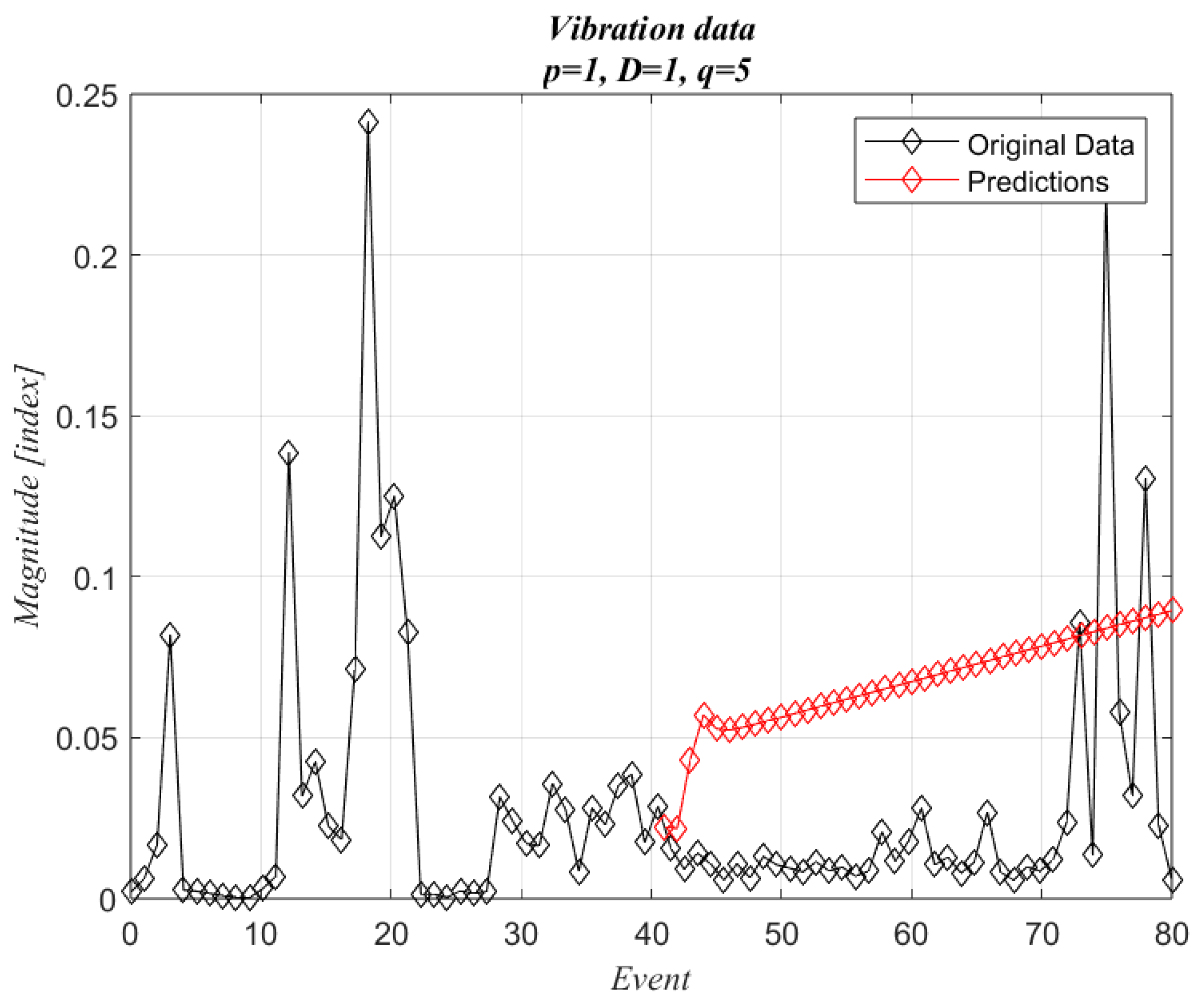
24]. The procedure started with setting D equal to one since there is no evident tendency. Then, p and q were selected at their minimum values. For measuring the likelihood, only 50% of the original data (1–40) were used for creating the prediction model, then the other 50% (41–80) were compared with the forecasting values. The lower q values are not included in this work; only the most significant results are presented, which correspond to q = 5.
Figure 9 shows the case when p = 1 and q = 5. Forecasted values (marked in red) show an increasing trend and neglect oscillations. This model is unable to predict wind fluctuations.
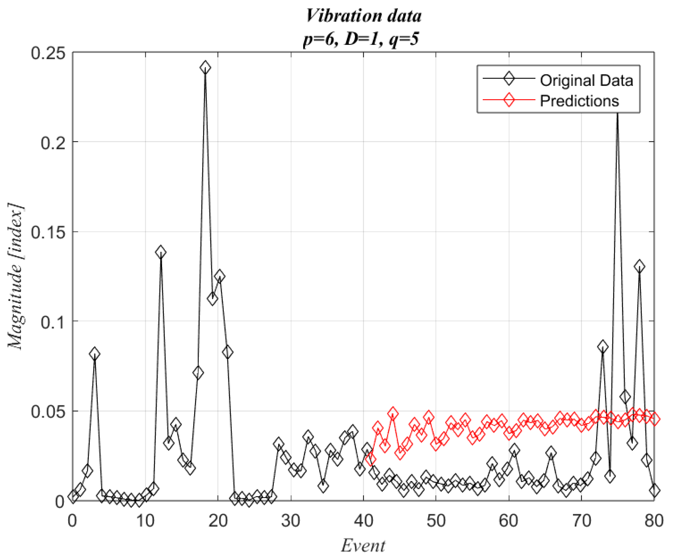
Figure 10 shows the results when p = 6, and
Figure 11 when p = 20. Both show wind variations, but
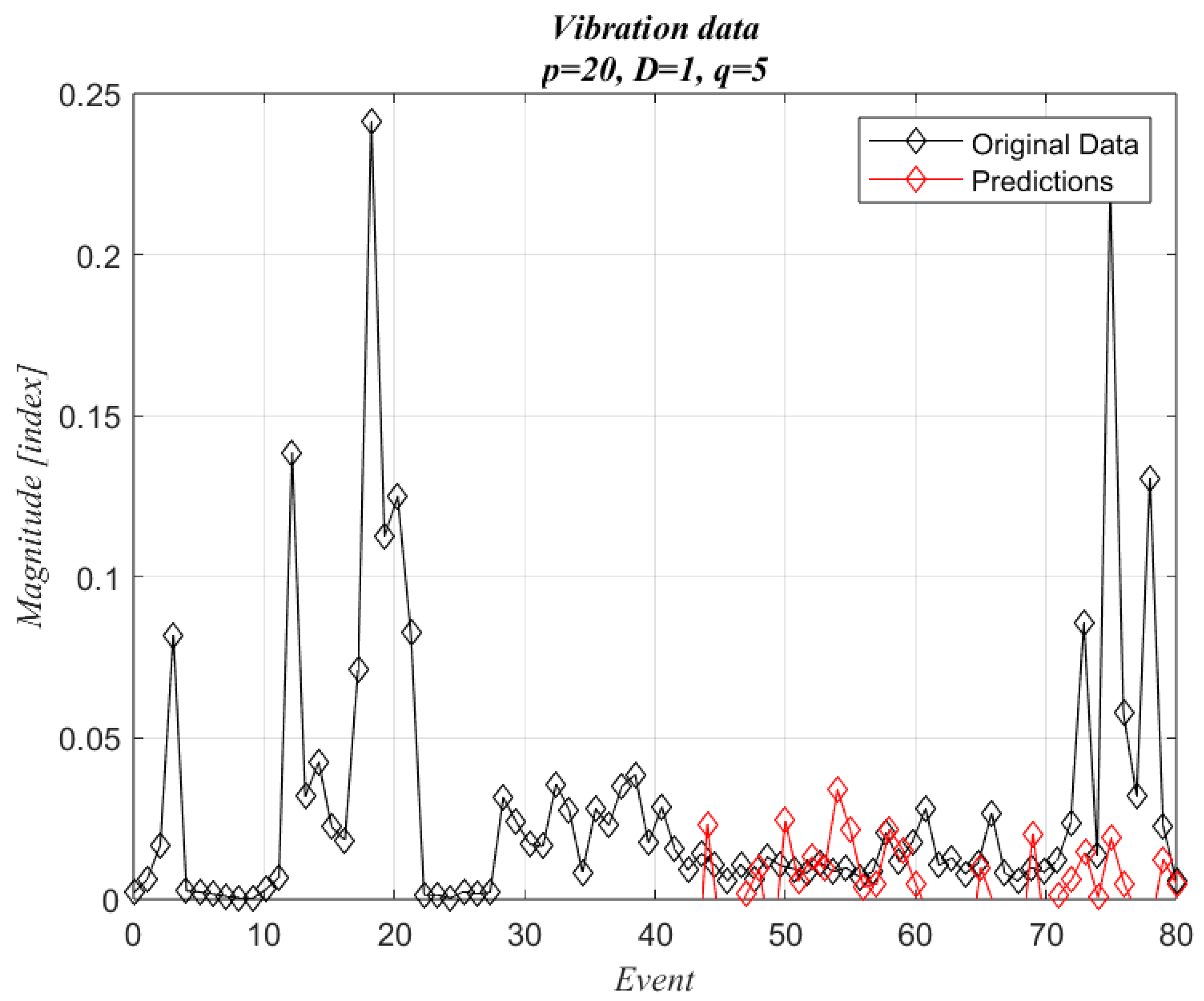
Figure 10 keeps a trend, and the predictions show larger values on average. The best approximation is shown in
Figure 11.
The final selection of the proper p and q values is obtained by plotting the variance between predictions and measurements. The graphical representation of variance versus p and q is shown in
Figure 12. It can be seen that the variance reduces rapidly with respect to q and has a smother behavior as a function of p. From this figure, the lower variance is obtained with p = 20 and q between 4 and 5. Thus, the best model is p = 20 and q = 5.
3.4. Predictions with the ARIMA Method
To assure that previous results are consistent, the ARIMA model was run with the full set of data, and it was used to forecast new operating conditions. The following table (
Table 1) shows the data analysis cases:
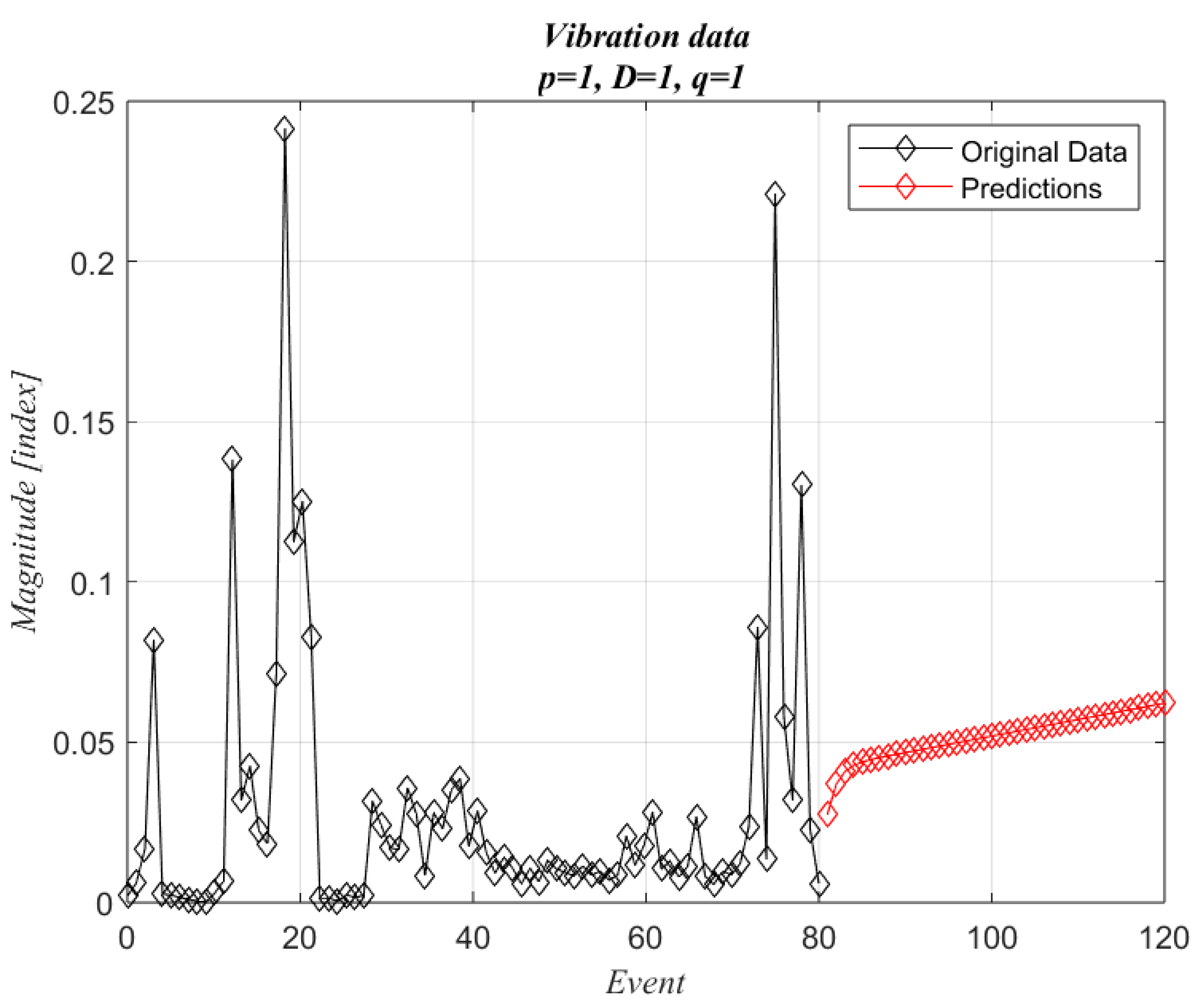
Case 1 is the simplest solution; the predictions will be constant, and the increments will be almost linear.
Figure 3 shows the original data with the forecasting values. The new values were estimated for an extra 40 events (50% of the original measured interval). The case with p = 1, and q = 1 did not produce any predictions. The differencing parameter did not contribute to improving predictions since it tried to smooth data with non-homogeneous variations. Predictions are similar to those obtained with 50% of the data (
Figure 13).
Case 2 (p = 10, d = 1, q = 1) shows predictions with oscillations and an incremental trend. Predictions look like a smooth function with no similarities with the original data (
Figure 14). Thus, the q parameter was incremented to two.
Case 3 (p = 10, d = 1, q = 2) also shows predictions with oscillations and an incremental trend. Predictions had a similar pattern to case 2 with an additional envelop function. (
Figure 15). Since the q parameter modified the overall results, it was incremented as described in the following cases.
Case 4 (p = 20, D = 1, q = 5) predictions show a similar pattern to the original data; there is no significant trend, and the only difference is a reduction in the amplitudes (
Figure 16). The slight trend is positive, which implies a natural tendency when forecasting damage in rotating machines. The resemblance to the original data and the slight trend confirms that these parameters are the best for forecasting the dynamic behavior of the wind turbine operating under gusty winds. The statistical analysis of this case is included in the
Appendix A.
The exponential forecasting method is the most accepted method for predicting the lifetime of rotating machinery [
25]. This method assumes that the vibration data (amplitudes of each frequency related to the rotating component) will behave as an exponential function. The function coefficients are calculated by fitting a regression curve from the historical data. The data is centered around the mode value, and the mode is determined from the histogram. The coefficients are recalculated every time that new data are recorded.
Figure 17 shows the original data and the forecasted estimations. The forecasted values only predict a simple progressive trend without considering sudden variations.


