Article

Motor Current-Based Degradation Modeling for Tool Wear Hybrid Prognostics in Turning Process

by
Atefeh Gavahian
1 and
Chris K Mechefske
2,*
1
Department of Electrical and Computing Engineering, Queen’s University, Kingston, ON K7L 3N6, Canada
2
Department of Mechanical and Materials Engineering, Queen’s University, Kingston, ON K7L 3N6, Canada
*
Author to whom correspondence should be addressed.
Machines 2023, 11(8), 781; https://doi.org/10.3390/machines11080781
Submission received: 30 June 2023 / Revised: 21 July 2023 / Accepted: 24 July 2023 / Published: 27 July 2023
(This article belongs to the Section Advanced Manufacturing)

Abstract

:
For many machines with turning process systems, the application of economical indirect Tool Condition Monitoring (TCM) is enhanced by utilizing internal encoder spindle motor current signals. In this study, we proposed a novel approach to extract the total harmonic distortion (THD) feature associated with the metal cutting frequency of a specific working tool in the time domain. Our method entailed the application of filtered variational mode decomposition (VMD) combined with envelope analysis to demodulate the motor current signal and define TCM features based on the THD of odd harmonics, which are more related to the motor structure. These features serve as inputs for a hybrid prognostics technique, employing the Geometric Brownian Motion (GBM) to stochastically model the degradation process along with a deep learning transformer-based framework called the time series Transformer (TST) to improve the life prediction. Finally, to validate our approach, we conducted experiments based on 36 sets of tool run-to-wear data extracted from a CNC machine operating under turning process conditions using two different tools. Finally, we compared the degradation models based on the extracted odd-THD and even-THD features.

1. Introduction

Lathe-based processes, such as turning and drilling, are performed as continuous machining operations that trim the workpiece from one spindle motor revolution to the next [1]. Among them, turning (also known as single-point cutting or fixed-tool machining [2]) is one of the most common machining processes in lathe-based production industries. In this process, the non-rotating cutting tool moves linearly toward and/or along the long axis of a rotating material bar (the workpiece). The geometry of inserting cutting tools mounted on non-rotating turrets is varied and sometimes complex. During the turning process with high-speed spindle rotations, the contact force between the tool and the workpiece results in gradually worn tool edges, which degrade the tool’s useful lifespan and may lower product quality [3,4]. Compared to other machining components, cutting tools typically experience a relatively short useful life; therefore, monitoring and predicting their condition prior to a damage level that results at the end of useful life can reduce the overall costs of system maintenance.
Tool condition monitoring (TCM) was introduced to correlate sensor systems and monitoring techniques to increase productivity by predicting tool deterioration levels. To indirectly measure tool wear evolution signals representing the cutting force, vibration, torque, spindle current or power, acoustic emission, motor stray flux [5], or a fusion of these signals can be used [6]. In the context of the drilling process [7], the electric power consumption of the main spindle emerged as a particularly intriguing element among multiple sensors for TCM. Among machining operations of TCM indicators, the spindle motor current was proven to be a cost-effective indirect measurement method that was correlated with main tool degradation process monitoring [8]. However, Ref. [9] shows that in the pre-stabilizing broaching process, the electrical current of the motors was found to be an irrelevant parameter for monitoring and did not provide any valuable insights into the tool condition. In this regard, enhancing broaching efficiency by combining offline indirect TCM with real-time monitoring techniques involved utilizing data from an accelerometer sensor alongside measurements of the cutting force, torque, and power from a servo motor during the cutting process. Notably, in the turning process, it showed that significantly more effort was required to address a lack of effective means for extracting and monitoring tool wear features using measured motor current signals, especially for fixed-tool processing [1,8,10,11,12].
The application of economical TCM in industrial settings using acquired internal encoder spindle motor current signals poses challenges due to the presence of distorted machine tool control actions and operation cycles, including concealed information within the noise and/or undesired data in the machining process [13]. The noise in time series signals can be effectively reduced through the utilization of signal processing techniques, such as decomposition algorithms [14] or wavelet transformation methods [15]. These methods allow for the extraction of desired signal components by separating them from unwanted noise components. Noise reduction methods can be extended to motor current signal analysis when an “air cutting” signal is available. The air-cutting signal represents machine behavior when the tool is not in contact with the workpiece and moves (as if cutting only air) until it encounters its next targeted metal surface. Additionally, in practice, the air-cutting signal is used for adjusting the numerical control program. It is acquired when the machine is run in the absence of a workpiece–tool interaction [13,16]. The difference between a normal cut and an air cut signal indicates the spindle motor current required for trimming metal [17,18]. In this study, we implemented a noise reduction technique by removing the frequency components associated with air cutting from the metal cutting signals along with employing decomposition methods to effectively reduce the noise level, specifically in the pure metal cutting state.
In order to serve as meaningful representations of the underlying tool condition, it is important to take the crucial step of extracting informative cutting features from the motor current signal. Motor current signature analysis (MCSA) offers a non-intrusive technique to extract relevant features, including amplitude, frequency contents, and related harmonics [19]. A noninvasive TCM technique has been proposed [20], which involves the extraction of features using the discrete wavelet transform (DWT) and time-frequency analysis of stray flux signals around the spindle motor. This work aims to establish a correlation between the cutting tool wear and the amplitude of motor stray flux harmonics. Another study [5] introduced a non-invasive methodology for diagnosing cutting tool wear in CNC machines by analyzing the stray flux and AC current signals from the spindle motor. An older study [21] explored the use of demodulation techniques, specifically the discrete wavelet transform, to extract features from the induction motor’s current signal to detect tool breakage in drilling operations.
Industrial time-series signals originating from any source encompass intricate and diverse modulation characteristics and are intricately tied to component faults through their associated modulating frequencies. These complex modulated signals arise from the combined influences of amplitude modulation (AM) due to time-varying transfer paths and frequency modulation (FM) effects. Therefore, demodulation techniques can be highly effective in this context, and a novel approach has been developed [22] that combines variational mode decomposition (VMD) with an empirical AM-FM amplitude and frequency modulation (AM-FM) decomposition methods to accurately estimate the instantaneous frequency of the vibration signal associated with planetary gearbox faults. In this regard, variational mode decomposition (VMD) for motor current feature extraction has been used to capture the nonstationary nature of the current signal, with ensemble learning (EL) to establish a nonlinear mapping between the extracted features and the tool wear level [14]. VMD is a time-frequency method for decomposing the nonstationary and nonlinear vibration signal of faulty gears into stable components [23]. Thereby, envelope demodulaton (envelope spectral analysis) can be applied to each VMD component to accurately extract features for the gear faults. Accurate fault detection and classification of Permanent Magnet Synchronous Motors (PMSMs) have been investigated [24] using stator phase currents. The suggested method integrated VMD, Hilbert-Huang Transform (HHT), and convolutional neural network (CNN) methods to autonomously analyze the characteristic behavior of the stator phase current signals and extract fault features based on frequency shifts and the instantaneous frequency. Another promising study [11] examined the nonlinear total harmonic distortion (THD) resulting from tool breakage and wear in the turning process. The experimental findings revealed that a significant increase occurred in odd harmonics at tool breakage, indicating their prevalence among unchanging and even harmonic frequencies.
Based on existing research into TCM methods [5,11,14,19,20,22,23,24], we have developed an innovative MCSA-based feature extraction technique. This indirectly examined the frequency characteristics of the motor current, which were influenced by the motor’s rotational speed during metal cutting. Our approach combined filtering, VMD, and envelope demodulation analysis to extract the time of the domain envelope features that were specifically relevant to the metal cutting frequency of each tool. By incorporating these envelope time domain features, degradation modeling for prognostics became more convenient and effective.
In order to progress beyond feature extraction and delve into tool prognostics as a key part of TCM, the subsequent phase involves constructing a predictive model that is capable of predicting the future condition of the cutting tools using the metal-cutting extracted features. The incorporation of failure history data, often known as run-to-failure data, holds significance in hybrid prognostics. In the context of TCM, the term run-to-wear is particularly relevant due to the possibility of reusing most tools by simply replacing their worn or broken operating edges. This historical dataset encompasses the temporal sequence of tool failures, offering invaluable insights into underlying degradation patterns and building a reliable prognostic framework for stochastic analysis [25].
Prognostics is a discipline that centers around understanding the progressive degradation of tool conditions over time and entails the estimation of the Remaining Useful Life (RUL) of tools [26]. Constructing models in prognostics can be broadly categorized into data-driven approaches [27], statistical model-based approaches [28], and hybrid approaches [29]. The hybrid prognostics approach has become increasingly popular for modeling degradation, as it combines the strengths of data-driven and statistical modeling techniques. This approach creates a powerful platform that can effectively capture the complex dynamics of degradation processes.
In the third family of prognostic methods, including hybrid prognostics, the degradation process is described by intelligently analyzing machine learning (ML) models that utilize available observations along with the foundations of stochastic processes. In degradation modeling, the objective is to capture the progression of degradation and predict the future behavior of the system or component. Stochastic processes, such as inverse Gussia and Gamma processes, are only used for monotonically increased degradation, whereas the Wiener process and its derivation from the Geometric Brownian Motion (GBM) [30] are commonly employed to model the non-monotonic fluctuations and uncertainties associated with positive degradation [31,32]. The stochastic process employed in degradation modeling assumes that the degradation follows a positive distribution, taking into account historical increments and volatility. However, it is important to acknowledge that relying solely on a stochastic process may not capture all non-linear dependencies in time series prediction tasks. Therefore, in the context of hybrid prognostics, incorporating advanced machine learning techniques can significantly enhance the accuracy and effectiveness of real-time prediction tasks in the prognostic domain. In recent years, machine learning approaches have broadened the scope of hybrid RUL prediction with multimode degradation mechanisms. Among them, Ref. [33] exhibits remarkable probabilistic incremental degradation within the latent space of the reconstruction-based Variational Autoencoders (VAE) prediction model. The learning process has been further enhanced by incorporating Generative Adversarial Networks (GAN). The recent advancements in VAE-based prognostics have demonstrated their efficacy in the field of industrial monitoring, as highlighted in the study referenced [34]. The hybrid prognostics approach with data augmentation used in [29] extends the concept of normalizing flows by dynamically transforming a continuous Wiener process as incremental modeling into a complex observable process through the use of dynamic instances of normalizing flows. Adversarial training can help mitigate the issue of overfitting and enhance the model’s robustness to some extent. However, GANs often encounter challenges such as mode collapse, unstable convergence, or gradient vanishing. Typically, these methods adopt the encoder-decoder architecture as their foundation. An alternative approach is the Transformer model [35], which has gained popularity for its effective utilization of self-attention in handling sequential representations. This model has been successfully employed as a time series transformer-based approach with several enhancements proposed in the literature [36,37,38].
Inspired by previous work, especially [11], this research proposes new features and properties for TCM. The remainder of this article is arranged as follows: Section 2 presents the definition of tool wear from the motor system perspective, discussing the effects of tool status on the motor current signal waveform. In Section 3, we delve into the methodologies employed for feature extraction, which include variational mode decomposition and envelope analysis. Afterward, we explore hybrid prognostics by combining GBM degradation modeling with the time series transformer (TST) prediction method. In Section 4, we provide a comprehensive overview of the experimental setup, including data definition, and present the results obtained from the conducted experiments for two different tools, focusing on prediction accuracy. Finally, in Section 5, we summarize the key findings and contributions of our proposed framework.

2. Definition of a Tool Wear Model Based on the Motor System

The motivation of this study is to confirm that motor current signals can indirectly capture tool status at early-stage failures. In the lathe turning process, multiple tools are held on a non-rotary tool holder (tool turret). Once a cutting tool is positioned for the cutting operation, it remains stationary while the workpiece rotates on the shaft of the sub-spindle motor, allowing the cutting action to occur, as presented in Figure 1. The question here is, how can the encoder motor current signal indirectly describe the tool damage levels during the cutting process where the tool is mounted at a constant position? The block diagram in Figure 1b describes the structure of the sub-spindle motor. If we treat the cutting tool process as a non-rotary load on the motor shaft, what effect does increasing the load (assuming the tool is worn and causes a non-rotary mild load on the three-phase spindle motor shaft) have on the motor current?
The load on an electric motor shaft, which is determined by the current it draws, is commonly referred to as the electric motor load. Changes in the amperage or rotational speed of the motor can be used to estimate this load. When the load is increased, it leads to a decrease in the back electromotive force (BEMF), resulting in a situation where the applied electromotive force (EMF) exceeds the BEMF. Consequently, more current is drawn by the motor to maintain the required torque. This creates a gradual increase in the speed difference between the motor’s field and rotor, which is known as the slip frequency. As a result of drawing an additional current through the stator windings and rotor bar, the motor experiences a progressive increase in temperature, potentially leading to overheating.
In the scenario where the load created by the worn tool falls within the safe range of the spindle motor, even under a no-load back-EMF condition, it can still impact the motor windings and the rotor bar, leading to an increase in rotor bar harmonics. In reference [39], it is asserted that in no-load motor conditions, the first-order and third-order harmonics of the BEMF are generated by the fifth and seventh harmonics of the air gap magnetic density, as well as the ninth and third harmonics, respectively. The study highlights the significance of the third and fifth harmonics of BEMF. Additionally, it suggests that a high amplitude of the output torque or current is a result of a large amplitude of the fundamental harmonic.
As the load on the motor increases, the motor speed initially decreases. This decrease in speed results in a reduction in the induced back electromotive force (BEMF) since BEMF and speed are inversely correlated. Consequently, if the BEMF is reduced, the current flowing through the motor also increases. This additional current provides the extra torque necessary for the motor to restore its speed under increased load conditions, as explained in reference [40]. Interestingly, the current waveform of the drive sub-spindle motor closely resembles the BEMF signal. As mentioned earlier, the BEMF waveform has a sinusoidal shape, and this eventually leads to the generation of the output harmonics of the third and fifth orders. Particularly, the current induced by the impression of reluctance slots has an air-gap flux density that carries the harmonic loss information of the rotor bars [41,42] and can be measured from the VMD of the sub-spindle motor current. Hence, this approach addresses the uncertainty in the motor current indicator for TCM mentioned in reference [11]. Moreover, it introduces a new THD indicator for monitoring the tool condition in the turning process by utilizing encoder data such as the current and motor speed.
T H D 3rd , 5th , = k = 3 , 5 , H I K I f u n d a m e n t a l 2
where, I K represents the amplitude of harmonics.

3. Methodologies

3.1. Feature Extraction

The preliminary stage of prognostics entails the critical task of extracting and selecting features that bear substantial degradation signatures with the objective of improving the efficiency and reliability of prognostic models. In TCM, it is important to reduce the costs associated with data and feature measurements [8,33].
Industrial systems commonly demonstrate a gradual degradation pattern rather than exhibiting abrupt and unexpected failures. Most ML-based prognostic models find it more convenient to analyze time-series data and features, preferably in time-domain signal processing [34]. Time-based signals facilitate the prompt detection of system status using elementary detection methods. Prominent time-domain feature engineering techniques, such as the root mean square (RMS), kurtosis, and crest factor, are commonly employed for analyzing and characterizing the signal, whereas the distribution of energy reflected in the spindle motor current bands signal can be observed by performing frequency-domain analysis while revealing a time-domain waveform comprising various frequencies. Furthermore, a correlation has been identified between the tool wear degree and the frequency-domain statistics of the motor current signal, as mentioned in [14].

3.1.1. Specific Challenges

During the processing of industrial data, motor current signals can pose significant challenges due to the presence of various types of noise sources in industrial settings, including electrical interference, environmental factors, and signal transmission issues. These challenges primarily involve the formation of a modulated signal during the process of metal cutting. This signal consists of multiple components that incorporate both amplitude modulation (AM) and frequency modulation (FM) features within a carrier signal.
  • Tool Cutting Frequency
The tool used to turn machine operations is prone to vibration due to its long and small diameter design. As the workpiece moves, the trajectory must conform to the shape, resulting in a change in its effective diameter when in contact with the workpiece, and the cutting speed varies slightly as well. The frequency at which a mounted tool passes through the rotating workpiece, known as the cutting frequency, is directly related to the spindle speed [43]. The tool cutting frequency is derived from the spindle speed and can be calculated using Equation (2).
M rpm = 60 × f c u t n
where M is the spindle speed (rpm), f c u t is the tool cutting frequency (Hz), and n is the number of tool edges, which in the turning process is n = 1 .
b.
Nature of Industrial Data
The nature of industrial motor current signals in the cutting process showcases a non-constant (non-linear) form of the carrier signal. This can be described in terms of modulation, where the essential vibration information of metal cuts is embedded into a time-varying carrier signal that is characterized by nonlinearity and noise (as illustrated in Figure 1). The waveform of the carrier signal in the motor current signal demonstrates temporal variations while serving as the carrier for modulated data, commonly referred to as the modulation signal.

3.1.2. Variational Mode Decomposition

In their pioneering work, Dragomiretskiy and Zosso [44] presented a groundbreaking time-frequency analysis technique called variational mode decomposition (VMD) that demonstrated exceptional proficiency in handling nonlinear and nonstationary signals. It also proved that it could overcome some limitations of the Empirical Mode Decomposition (EMD) method, such as mode mixing and end effects [21].
VMD is a non-recursive decomposition method that excels in extracting distinct stationary AM-FM components from non-stationary multi-component signals x t both adaptively and concurrently. The intrinsic mode functions (IMFs) can be regarded as explicit AM-FM models, wherein the bandwidth of each IMF is directly associated with the parameters of the AM-FM models. Each IMF m o d e k t = m o d e 1 ,     ,   m o d e k is defined by a limited bandwidth that is centered around its corresponding central frequency of ω k = ω 1 ,     ,   ω k . As the VMD algorithm iteratively updates each m o d e k in the frequency domain and determines the ω k , all IMFs mostly compact around the central frequency, reflecting their distinct sparsity properties of them [21,22,23,24].
The shape of IMFs that possess both amplitude and frequency modulation characteristics can be expressed in Equation (3).
m o d e k t = A k t c o s ϕ t
In the given equation, A k t is the non-negative envelope amplitude modulation signal and ϕ t   denotes the instantaneous phase resulting from the frequency modulation with a positive derivative known as instantaneous central frequency ( ω k t = d   ϕ t d t > 0 ).
m i n m o d e k ,   ω k = K t { δ t + j π t m o d e k t }   e j ω k t 2 2
L m o d e k ,   ω k , λ = γ   K t { δ t + j π t m o d e k t }   e j ω k t 2 2 + f t K m o d e k t 2 2 + λ t , f t k = 1 K m o d e k t
Equation (4) computes the optimal minimum of the VMD through a series of the iterative sub-optimization algorithm to find the augmented Lagrange saddle-point, in which λ t is the time-varying Lagrange multiplier and γ is the penalty factor to balance the constraint of the data-fidelity. The saddle-point as the optimal solution of our model, is continuously updating m o d e k n + 1 ,   ω k n + 1 and λ n + 1 .
m o d e k n + 1 = a r g m i n m o d e k γ k t { δ t + j π t m o d e k t }   e j ω k t 2 2 + f t k m o d e k t 2 2
The transformation of Equation (6) into the refreshing frequency domain, and the corresponding central frequency can be performed using Equation (7), respectively [32].
m o d e ^ k n + 1 ω = f ^ ω i k m o d e i ^ ω + λ ( ^ ω ) 2 1 + 2 γ ω ω k 2   and , ω k n + 1 = 0 ω m o d e k ^ ω 2 d ω 0 m o d e k ^ ω 2 d ω
where m o d e ^ k n + 1 ω denotes the winner filter of the motor current residual f ^ ω i k m o d e i ^ ω   and the power spectrum of motor current mode is obtained from the ω k n + 1 term. The completed VMD procedure is summarized in Table 1.
VMD effectively decomposes the signal into a specific number of IMFs, allowing for the estimation of their amplitude envelope and instantaneous frequency.

3.1.3. Empirical Envelope Amplitude and Spectrum Analysis

In this study, accurate features that enhance the performance of the MCSA-TCM algorithm are introduced by improving VMD reconstruction signals, which are derived from selected IMFs within the metal cutting frequency fluctuations and their harmonics. According to prior knowledge about the nature of AM-FM IMFs, the carrier signal of the IMF must be separated from this contamination to estimate the instantaneous frequency. To identify the modulation characteristics of each mode, a Hilbert transform is applied to separate the Frequency Modulation (FM) term, which represents the instantaneous frequency variations, from the Amplitude Modulation term [22,45]. The first step in calculating the instantaneous frequency for each IMF is to split the amplitude envelope and carrier signal using the Normalizing Hilbert transform [22]. The instantaneous frequency is then calculated by evaluating the local phase derivative of the carrier signal, as shown in Equation (8).
f t i n s t = 1 2 π   d d t a r c t a n H C a r r i e r t C a r r i e r t
As a second step, we selected the envelope spectra of IMFs with the median within the metal cutting frequency range of each tool to reconstruct the motor current signal in the metal cutting process. The process of reconstructing the motor current signal was performed by selecting the envelope spectrum of IMFs with the median f t i n s t in the metal cutting frequency range for each tool. This allowed reconstructed signals to hold the maximum wear symptoms of the processing tool. Finally, to enhance the representation of this feature for subsequent incremental modeling, we employed Inverse Fast Fourier Transform (IFFT) to transform the feature into the time domain, resulting in an Envelope representation.

3.2. Degradation Modeling and Prognostics

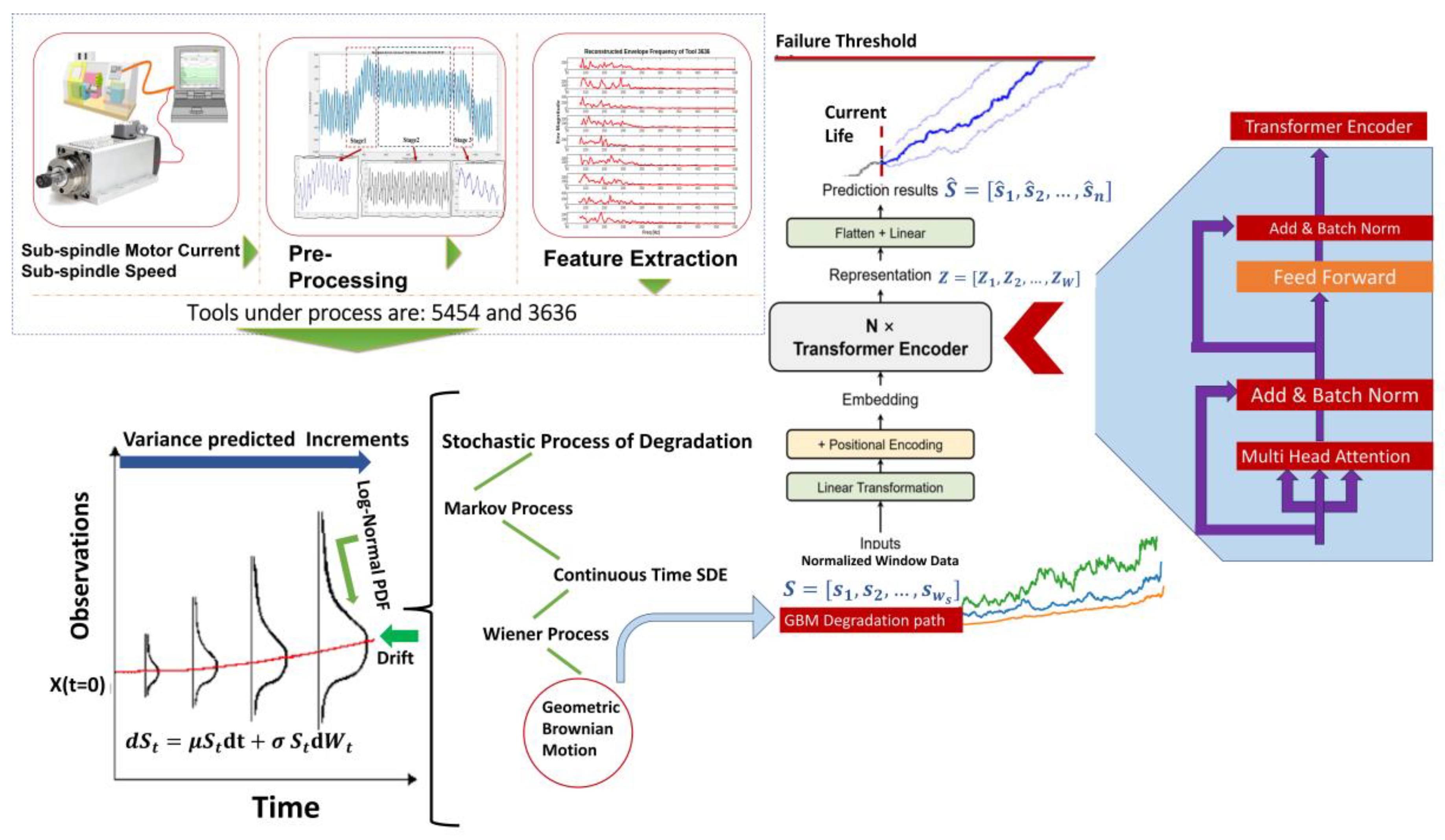
In order to demonstrate the real-time TCM, the next stage was to model the incremental behavior of our features. In the hybrid prognostics techniques, probabilistic methods such as the Wiener process or Gamma process [46,47,48] are used to stochastically model and predict the increments of a time series signal. In order to increase the performance of stochastic processes, ML-based methods are used widely. In this regard, we redesigned the continuous stochastic process of the Geometric Brownian Motion (GBM) structure incorporating the ML-prediction technique. The prediction method is a novel method called a Transformer-based Framework, which is derived from the latent space of the Normalizing Flow (NF) network concept [49].

3.2.1. GBM in Brief

GBM, or the Geometric Brownian Motion, is a stochastic differential equation (SDE) (Figure 2) that is commonly used as a non-monotonic incremental process for prognostics or degradation modeling. It serves as a mathematical framework to describe the evolution of a system’s degradation over time. It assumes that the degradation follows a continuous time process that exhibits random fluctuations similar to the Brownian motion [29]. The Langevin SDE is shown in Equation (9).
X t = X 0   e ( μ σ 2 2 ) t + σ W t , X 0 = X 0
Then, the log-normal probability distribution function of X t , f x t x ; μ _ , σ _ , t   with μ _ = μ σ 2 2 and σ _ = σ t returns its future increments as:
f x t x ; μ _ , σ _ , t   = 1 x 2 π t σ 2 t × e x p ( l o g   x l o g   μ   ¯ t     2 σ _ ) ,
The log-normal distribution ensures that the values of the degradation variable remain positive and accommodate asymmetry in the distribution. The GBM, as a stochastic process, has a deterministic drift and a volatility term that produces a random fluctuation. This fluctuation mode f x t that represents the unpredictable changes in increments based on their random nature, as denoted by x = e ( μ t 3 σ 2 t 2 ) , with inflection points at x = e [ μ σ 2 t ± σ σ 2 t 2 + 4 t 2 ] . The GBM itself is useful for modeling the stochastic nature of historical degradation paths; however, there may exist dependencies that influence the prediction process, which GBM fails to account for independently.
The fluctuation mode of f x t is denoted by x = e x p ( μ t 3 σ 2 t 2 ) , with infliction points at x = e x p [ μ σ 2 t ± σ σ 2 t 2 + 4 t 2 ] .

3.2.2. The Time Series Transformer Prediction

The stochastic process assumes that the degradation follows a positive distribution using a historical increment and volatility. However, there could be other nonlinear dependencies that impact the degradation process and are not captured by GBM alone. In this regard, by incorporating a deep machine learning method [36], we increased the capabilities of GBM. The time series transformer-based framework [50], which was built upon the transformer encoder architecture introduced for multivariate time series representation learning together with degradation modeling, created a robust hybrid prognostics platform capable of accurately predicting the growth of wear (Figure 2).
Let us consider windowed GBM paths as S ϵ R w s × m = s 1 , s 2 , , s w s , where w s is a look-back window length with m variables. To begin the processing, the feature vectors are first transformed through linear mapping into a d-dimensional space with the help of learner parameters of w P and b P :
  u t = w P s t + b P
In the transformer architecture, the feed-forward network and the multi-head self-attention components do not naturally take into account the sequential nature of input data. This means that the model does not have an inherent understanding of the temporal order in which the data points occur. Instead, positional encodings are introduced and provide the model with information about the relative positions of data points in the input sequence. In the case of time series data, sinusoidal encodings are commonly used. These encodings assign unique values to different positions in the sequence, allowing the model to recognize temporal patterns and dependencies [38]. Then, the multi-head self-attention mechanism U Q , K , v in TST can be implemented similarly to the Transformer architecture. It allows the model to attend to different parts of input data and capture relevant temporal dependencies. The matrix U Q , K , v is derived from U t = u 1 , u 2 , , u w s and the position of encoding w P o s , as U Q , K , v = U + w P o s . This layer generates queries Q = U Q , K , v × w Q , keys K = U Q , K , v × w K , and values v = U Q , K , v × w v for the multi-head self-attention layer with the learnable parameter of w Q , w K , w v .
When multiple attention heads are employed, outputs are then concatenated together, resulting in a combined representation that captures diverse patterns and dependencies in input data which are mapped to the encoder section. Following the self-attention operations carried out by the Transformer’s encoder, the latent representation vectors z t ϵ R d derived from Equation (12), resulting from each time step are reshaped into a one-dimensional vector of   z ¯ ϵ R d .
  Ζ = S o f t m a x 1 d × Q K T × v
The flattened latent output is passed through a linear layer to match the target output required for the prediction task:
  S ^ = w P r e d Ζ + b P r e d
where S ^ , w P r e d R n × w s × d and b P r e d R n are the prediction of S and the learner variables, respectively, of n prediction steps.

4. Experimental Setup and Results

The experiment was conducted on the sub-spindle motor current and the speed signal of an industrial CNC machine during the turning process, in which the motor is a four-pole, three-phase AC synchronous servo of the Fanuc-A06B-1444-B103-AC model with Spindle-Motor B-3-1000i-3-7kW-5HP. The data are recorded within the FANUC controller and SERVO VIEWER, which is tailored for machine tools equipped with FANUC CNC systems. Its primary function is to precisely measure, record, and monitor servo/spindle data, encompassing essential parameters such as motor currents, positioning, speed, and torque. The sub-spindle motor, powered by a beta iSVSP servo amplifier, is a three-phase AC synchronous servo motor with four poles. Connecting the motor directly to the industrial power source could result in the burning out of its windings. Therefore, it is crucial to exclusively use the designated amplifier for power supply. The servo amplifier eventually eliminates the 60 Hz frequency. The motor operates by rotating a screw-like shaft to facilitate linear movement at the spindle shaft, effectively converting a non-linear input into a linear motion. It is important to note that the industrial production process used to collect the data used does not involve any external or additional sensors or connections. It is a standard procedure in a production environment.
In this study, we examined two different tools with assigned numbers T3636 and T5454. During their distinct cutting processes, they shaped the workpiece differently. In the lathe process, the AC servo motor operated at around 5000 rpm (or 83.33 Hz) and 3000 rpm (or 50Hz) while using tool number 5454. This specific tool is considered a nonlinear external load, causing abrupt changes in the output current. The dataset collected over 32 days represented 32 sets of the run-to-wear data, where each set corresponded to a specific cutting process of two tools performed until the tool wore out, 29 sets for tool 5454 and the rest for tool 3636. Once the tool reached a worn-out state, the operator would typically adjust the tool position or replace the tool. The provided data are in the form of *.mat files, with a save interval of 2 min. The data include information on two different tools: Tool 5454 and Tool 3636. Tool 5454 consisted of four cutting processes, while Tool 3636 had nine cutting processes. All the processes for conducting the analysis in Python and the Visual Studio Code (VScode) framework were carried out within the ComputeCanada computing environment.

Data Preprocessing

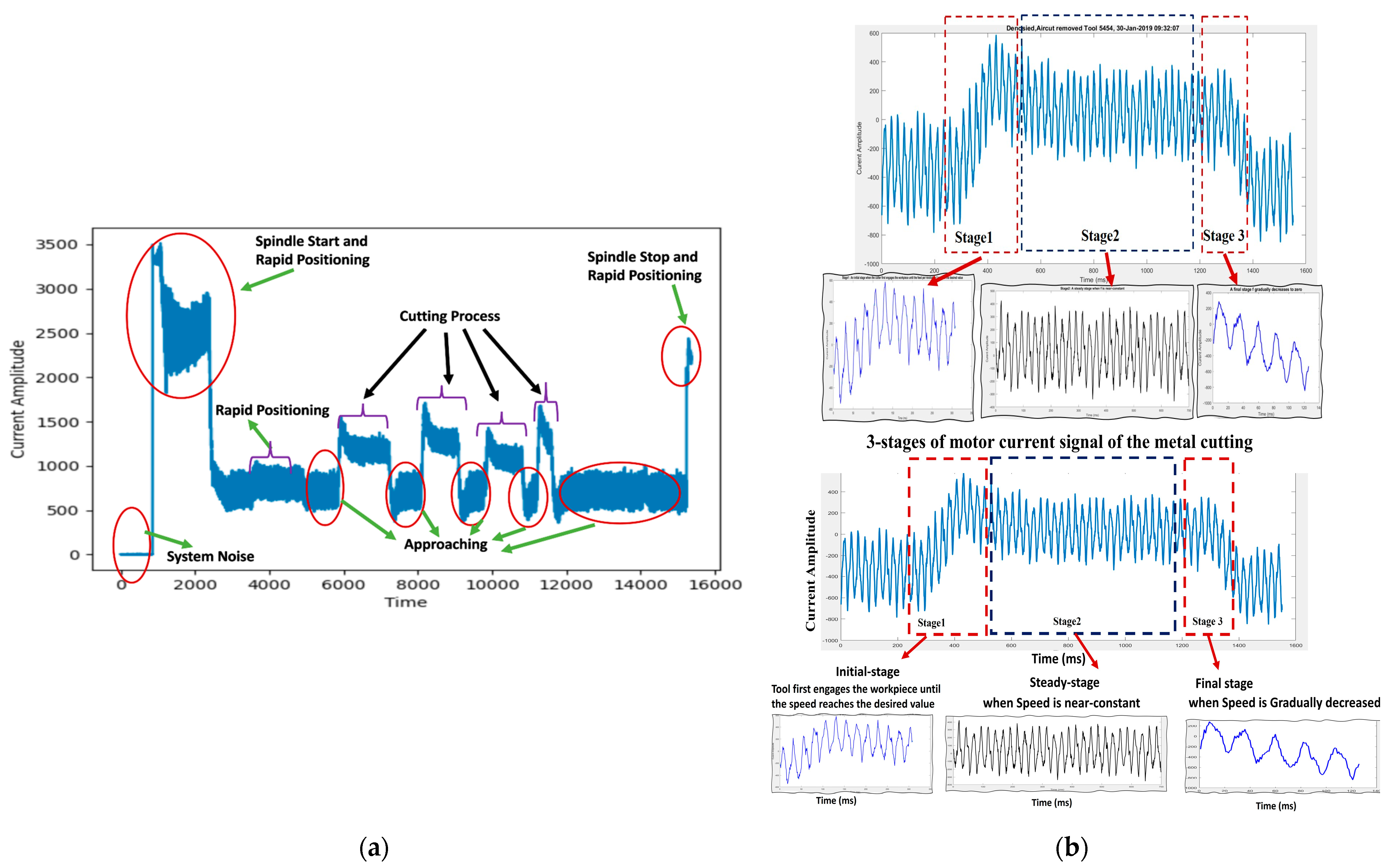
Figure 3a illustrates that not every part of the turning process contained useful information about the tool condition of the raw motor current signal. Instead, specific segments of the signal carry relevant information. The important parts are as follows.
(a)
Active Cutting Movement: So-called cutting process, this segment refers to the period when the cutting tool is actively engaged with the workpiece, resulting in material removal.
(b)
Passive Cutting Movement: So-called approaching process during this phase, the spindle rotates at the same speed, and the tool turret is distanced from the workpiece. It can be considered an “Air Cut” signal, where the cutting tool is not in contact with the workpiece.
(c)
System Noise: In the absence of active positioning and the turning of the sub-spindle, certain noise components may be present in the signal. This noise can originate from various sources, such as cables or sensors, and may introduce unwanted variations in the signal.
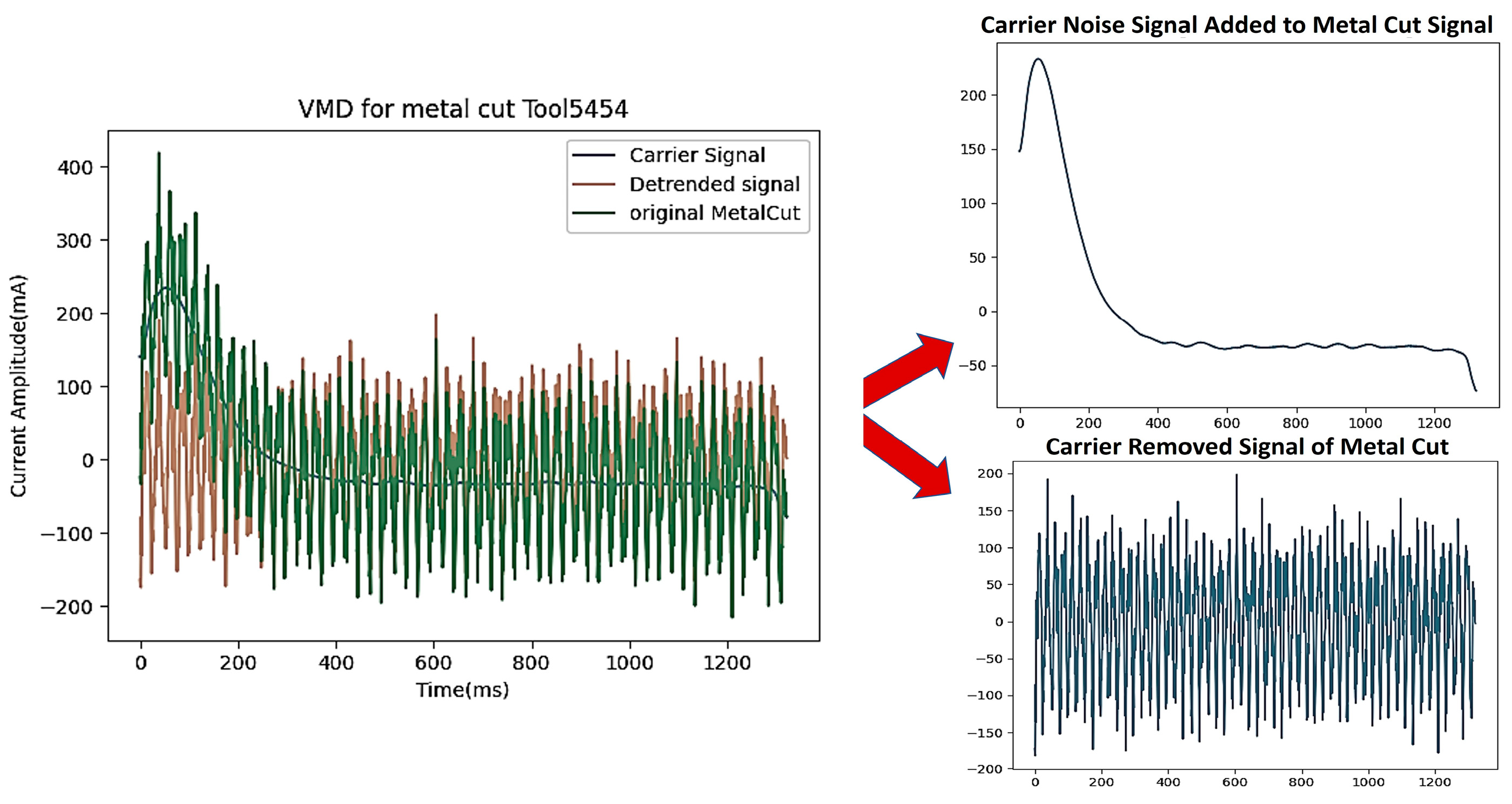
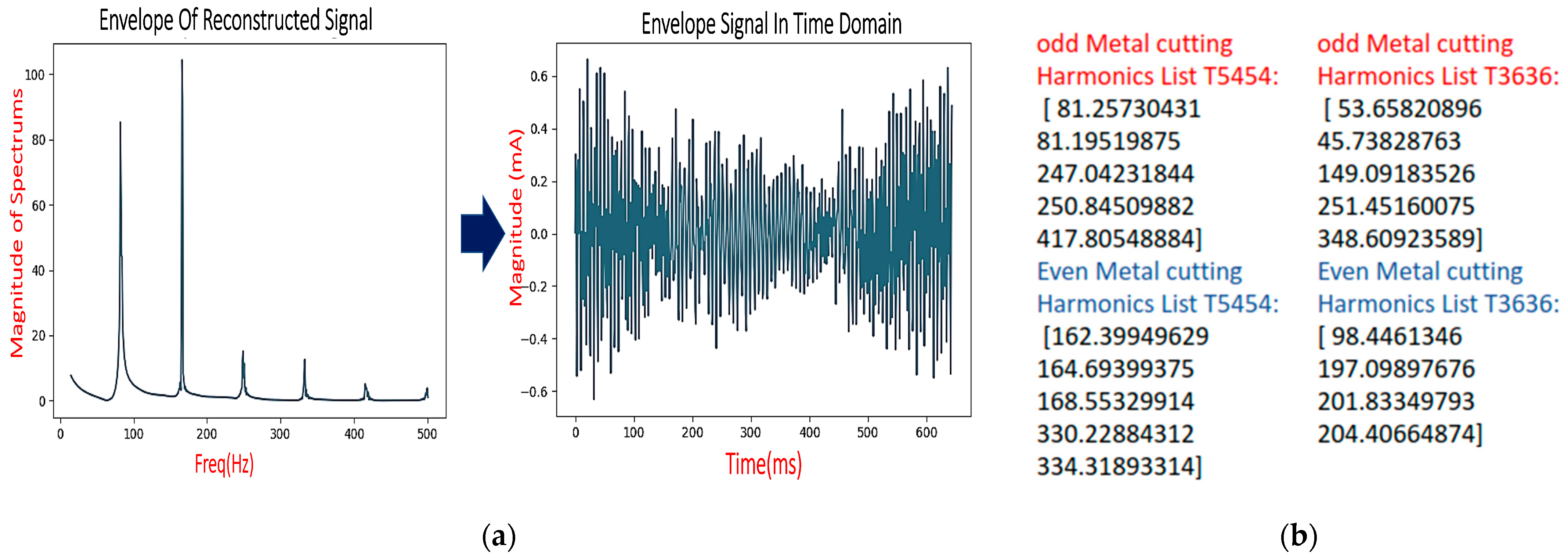
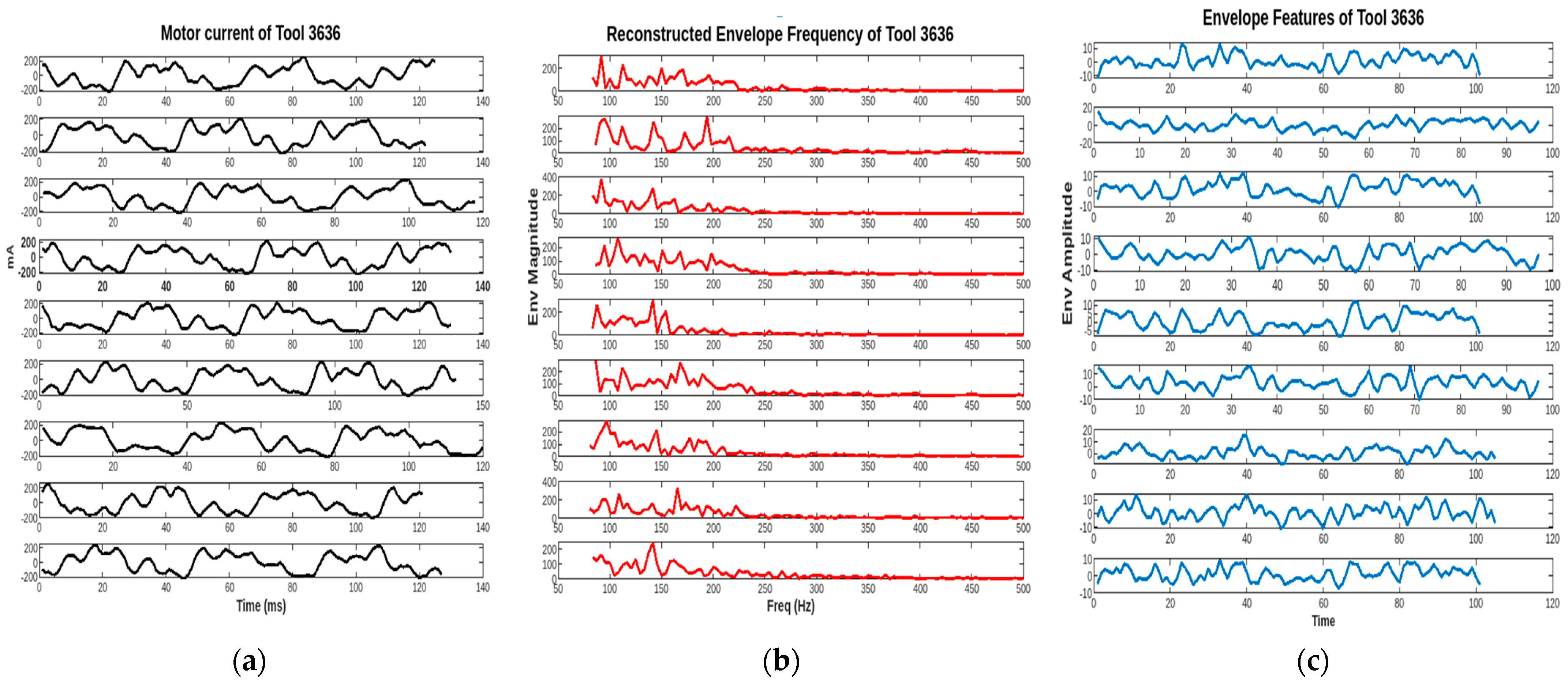
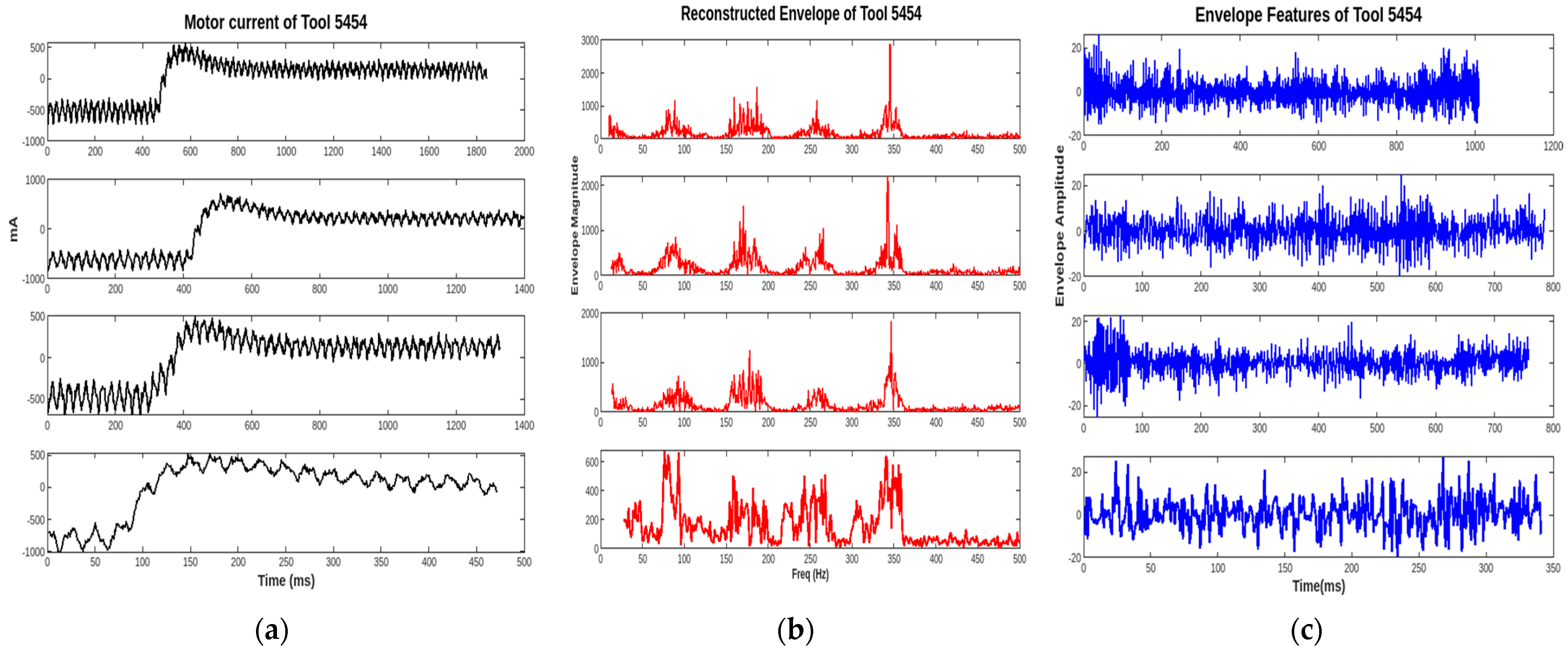
In a turning machine, when the insert tool is not cutting in its optimal conditions, it generates a variation in the current that is required by the spindle motor. As mentioned, the subtraction executed on the current signal from normal and air-cut results helps provide a clear signal for further processing. Moreover, the interaction of the cutting process from the first stage onward has made changes in the spindle motor current signal, where each part of the current signal can be assigned to a certain stage. To increase the accuracy of analysis, in this paper, each cut was divided into three predefined stages (Figure 3b). In order to extract the time domain data that include more likely related frequencies of tool fault growth, we calculated the cutting frequency for Tool 5454 and Tool 3636 are 83.33Hz and 50Hz, respectively, which is the same as their fundamental frequencies. Based on [8], the total harmonic distortion for odd harmonics only could carry information for early fault detection. In the process of reconstructing the motor current signal containing the fault growth frequencies, the first stage was to remove the carrier signal, as shown in Figure 4. In the VMD analysis, the embedded filter within the method was designed to capture the relevant harmonics associated with the range of changes in the frequency of the motor speed during the metal-cutting process. To reconstruct the motor current signal, all the decomposed IMFs with central frequencies around the harmonics were captured. Eventually, the empirical envelope amplitude and spectrum analysis was performed to reconstruct the metal cutting process (Figure 5).
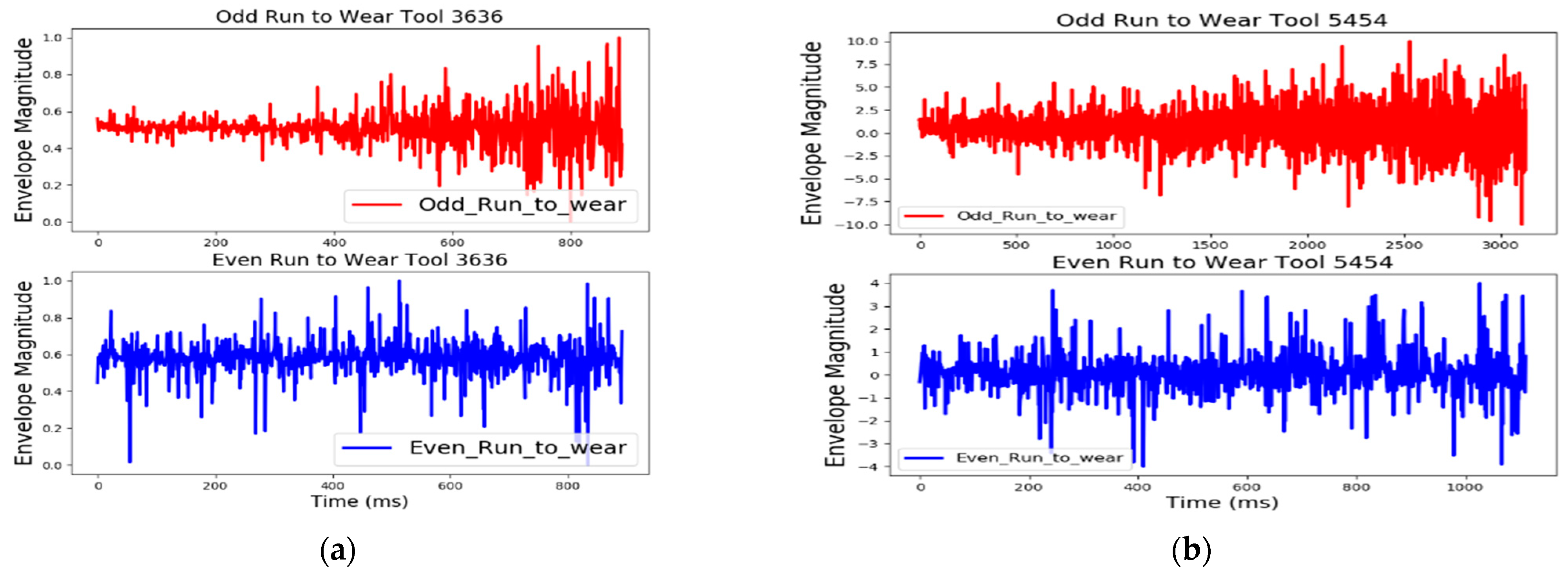
The proposed features are presented in Figure 6 and Figure 7 for Tool 336 and Tool 5454, respectively. The comparison of extracted features for each tool reveals an interesting finding: the THD of the odd harmonics for cutting frequencies exhibited a significantly larger envelope magnitude compared to the THD of the even harmonics. This indicates that in the turning process, the odd harmonics of the cutting frequency played a more prominent role and were stronger candidates for indirect Tool Condition Monitoring (TCM). The comparison results, as depicted in Figure 8, clearly demonstrate that our study successfully identified and extracted appropriate features that captured the characteristics of the cutting frequencies for each tool in the turning process. Specifically, for both Tool 3636 and Tool 5454, the THD of the odd harmonics stood out, emphasizing its significance in detecting and monitoring the tool condition indirectly through TCM methods from a healthy state up to the wear, Figure 9.
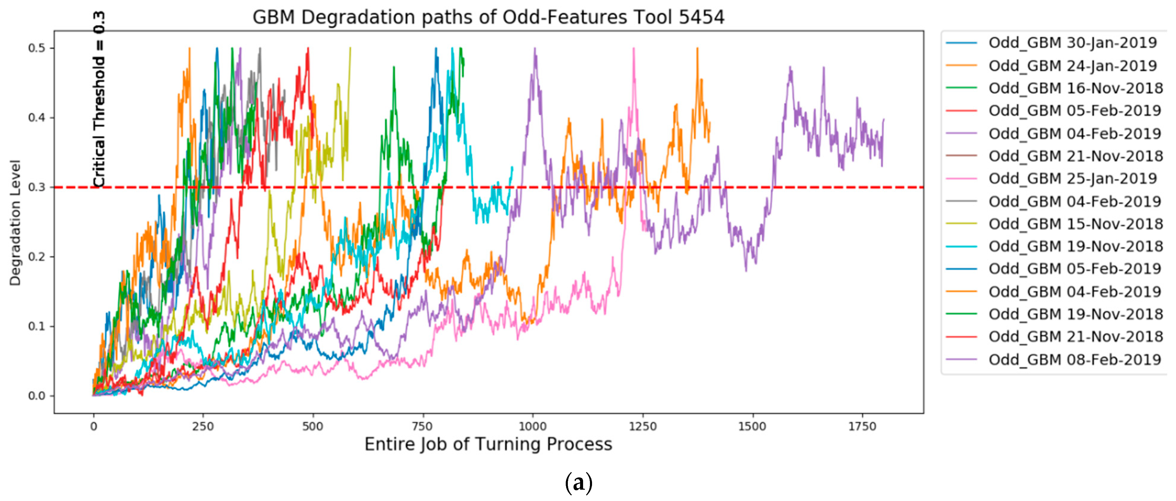
By extracting the entire run-to-wear process of the metal cutting, we observed a consistent pattern and a progressive increase in the amplitude of the motor current leading up to failure in relation to the envelope THD odd harmonics. By contrast, the THD of even harmonics displayed a fluctuating behavior with comparatively lower amplitudes. This gradual degradation time-series pattern observed in Figure 10 across the turning processes demonstrated the more pronounced degradation of Tool 5454 compared to Tool 3636. Following the implementation of our hybrid prognostics method, we stochastically modeled the degradation growth for each on historical run-to-wear process using GBM.
The incorporation of random walk modeling, along with the proposed odd features, demonstrated the effectiveness of indirectly assessing TCM in the machine turning processes. However, the growth pattern of the other even features followed a random walk order but failed to reach the predetermined threshold. Moreover, when considering the entire total harmonic distortion comprising both odd and even harmonics, its influence on assessing the tool condition was significantly minimal. This observation aligns with existing findings in the relevant technical literature. The GBM modeled the degradation through the random walk increments of our data, and based on observation, we set a critical threshold of C = 0.3 in each path (Figure 11 and Figure 12).
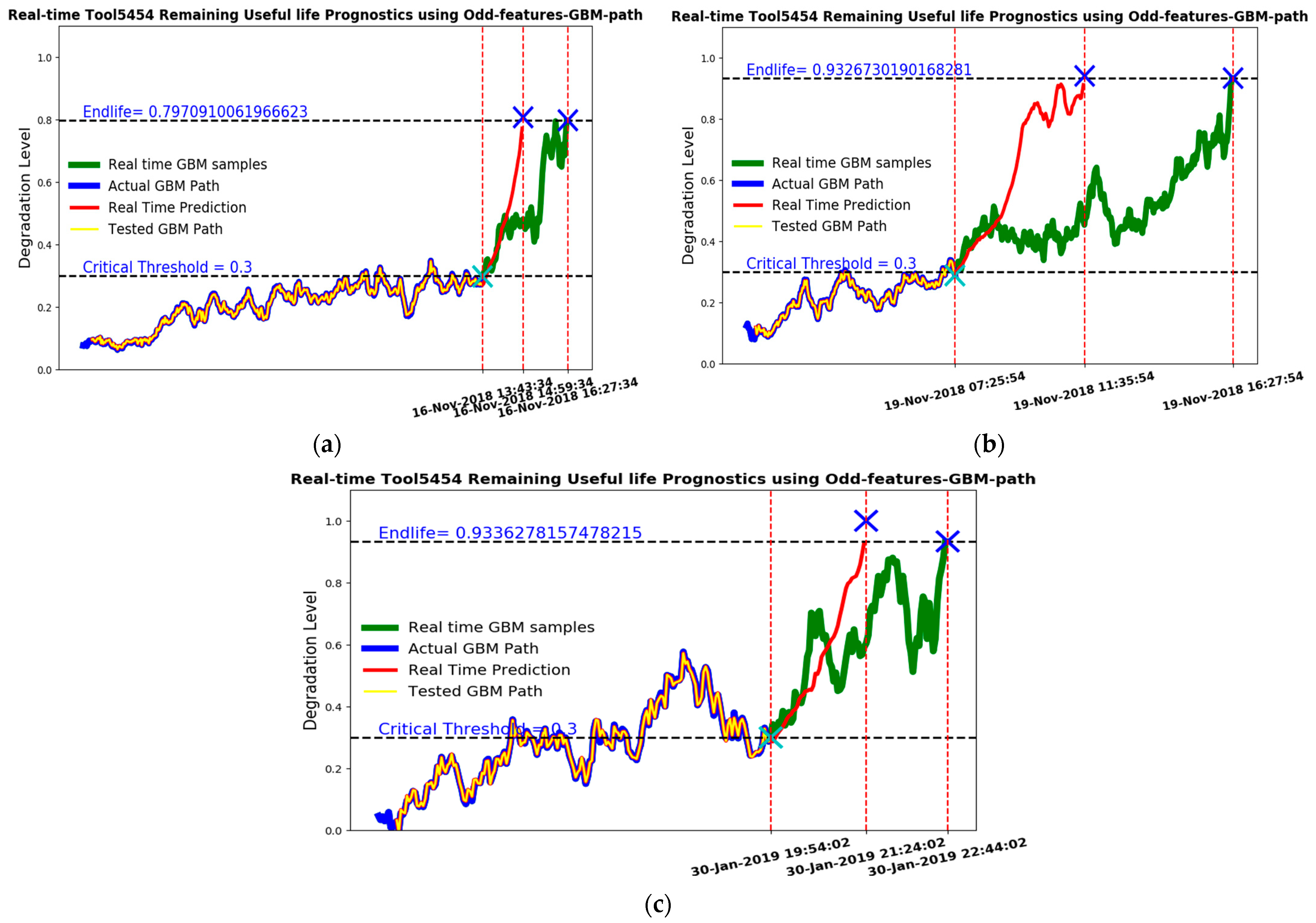
To extend our method for prediction, we employed the time series transformer model to the odd features of Tool5454 and Tool3636. By training the transformer on the historical degradation paths until the threshold and incorporating this into the hybrid prognostics framework, we could predict future degradation growth and estimate the remaining useful life of the tools. In order to address the limitations posed by even features, our prediction model was trained exclusively on the 27 run-to-wear paths of both tools, focusing solely on their odd features. Figure 13 demonstrates the convergence process of the TST model training. To optimize CPU usage, we chose to limit the number of epochs to 28. This decision helped minimize the computational load and enhance the efficiency of the training process. To evaluate the model’s performance, we utilized nine sets of similar type paths for testing and validation purposes. The prediction model was tested using a real-time setup with a window size of 10. The validation results demonstrated that the model’s prediction path successfully forecasted an adequate remaining useful life cycle. As evident from Table 2, each prediction cycle had a duration of 2 min. Figure 14 and Figure 15 illustrate the prognostics for Tool 5454 and Tool 3636, respectively. By establishing a critical threshold, denoted as C, we defined the tool’s end-life as the run_to_wear path’s endpoints. We expressed the lifetime of the tool, denoted as T, through Equation (12) to estimate the remaining lifespan of the tool before it reached its end-life.
T = i n f t : X t C | X 0 < C

5. Conclusions

This study presents a novel approach to enhance economical indirect TCM in machining with turning process systems. This method involves extracting odd and even harmonic distortion features from the spindle motor current signal and specifically targeting the application of VMD as a filtered demodulation technique within envelope analysis. The resulting TCM features based on the THD of odd harmonics can be closely related to the motor structure and are compared at different stages of tool wear. The THD features to serve as an input for a hybrid prognostics technique, incorporating the Geometric Brownian Motion for stochastic degradation modeling within critical and end-life thresholds of the tool.
Experiments were conducted on 36 run-to-wear datasets from a CNC machine under turning process conditions with two different tools. The proposed features demonstrated the potential for cost-effective TCM in machining systems and provided insights for developing advanced prognostic techniques for tool life prediction. This study implemented a machine learning transformer-based framework to train and test the prognostics model using 27 complete run-to-wear paths. The validation results were highly satisfactory, as the provided RUL enabled the timely replacements of degrading tools before reaching critical wear levels.
In conclusion, the developed hybrid prognostics method effectively leverages the proposed odd features extracted from the sub-spindle motor current for TCM tasks. This technically advanced approach offers real-time monitoring and prediction of tool degradation, thereby enhancing the overall performance and efficiency of the turning process.

Author Contributions

Conceptualization, methodology, software, validation, formal analysis, investigation, data curation, writing—original draft preparation, A.G.; writing—review and editing, A.G. and C.K.M.; resources, supervision, project administration, C.K.M. All authors have read and agreed to the published version of the manuscript.

Funding

This research received no external funding.

Data Availability Statement

Not applicable.

Acknowledgments

This research was supported by the Natural Sciences and Engineering Research Council of Canada and the Digital Research Alliance of Canada.

Conflicts of Interest

The authors declare no conflict of interest.

References

  1. Zhou, Y.; Sun, W. Tool Wear Condition Monitoring in Milling Process Based on Current Sensors. IEEE Access 2020, 8, 95491–95502. [Google Scholar] [CrossRef]
  2. Trimantec. Machining Processes Overview. Available online: https://trimantec.com/blogs/t/machining-processes-overview (accessed on 14 August 2020).
  3. Gajate, A.; Haber, R.; del Toro, R.; Vega, P.; Bustillo, A. Tool wear monitoring using neuro-fuzzy techniques: A comparative study in a turning process. J. Intell. Manuf. 2012, 23, 869–882. [Google Scholar]
  4. Bagga, P.; Makhesana, M.; Patel, H.; Patel, K. Indirect method of tool wear measurement and prediction using ANN network in machining process. Mater. Today Proc. 2021, 44, 1549–1554. [Google Scholar] [CrossRef]
  5. Jaen-Cuellar, A.Y.; Osornio-Ríos, R.A.; Trejo-Hernández, M.; Zamudio-Ramírez, I.; Díaz-Saldaña, G.; Pacheco-Guerrero, J.P.; Antonino-Daviu, J.A. System for Tool-Wear Condition Monitoring in CNC Machines under Variations of Cutting Parameter Based on Fusion Stray Flux-Current Processing. Sensors 2021, 21, 8431. [Google Scholar] [CrossRef] [PubMed]
  6. Aghazadeh, F.; Tahan, A.; Thomas, M. Tool condition monitoring using spectral subtraction and convolutional neural networks in milling process. Int. J. Adv. Manuf. Technol. 2018, 98, 3217–3227. [Google Scholar] [CrossRef]
  7. lvarez-Alcón, M.; López de Lacalle, L.N.; Fernández-Zacarías, F. Multiple sensor monitoring of CFRP drilling to define cutting parameters sensitivity on surface roughness, cylindricity and diameter. Materials 2020, 13, 2796. [Google Scholar] [CrossRef] [PubMed]
  8. Kuntoğlu, M.; Aslan, A.; Pimenov, D.Y.; Usca, Ü.A.; Salur, E.; Gupta, M.K.; Mikolajczyk, T.; Giasin, K.; Kapłonek, W.; Sharma, S. A Review of Indirect Tool Condition Monitoring Systems and Decision-Making Methods in Turning: Critical Analysis and Trends. Sensors 2020, 21, 108. [Google Scholar] [CrossRef]
  9. Del Olmo, A.; De Lacalle, L.L.; De Pissón, G.M.; Pérez-Salinas, C.; Ealo, J.A.; Sastoque, L.; Fernandes, M.H. Tool wear monitoring of high-speed broaching process with carbide tools to reduce production errors. Mech. Syst. Signal Process. 2022, 172, 109003. [Google Scholar] [CrossRef]
  10. Kuntoğlu, M.; Sağlam, H. Investigation of signal behaviors for sensor fusion with tool condition monitoring system in turning. Measurement 2021, 173, 108582. [Google Scholar] [CrossRef]
  11. Akbari, A.; Danesh, M.; Khalili, K. A method based on spindle motor current harmonic distortion measurements for tool wear monitoring. J. Braz. Soc. Mech. Sci. Eng. 2017, 39, 5049–5055. [Google Scholar] [CrossRef]
  12. von Hahn, T.; Mechefske, C.K. Machine Learning in CNC Machining: Best Practices. Machines 2022, 10, 1233. [Google Scholar]
  13. Repo, J.; Wretland, A.; Beno, T.; Tu, J. In-Process Tool Wear Detection Using Internal Encoder Signals for Unmanned Robust Machining. High Speed Mach. 2016, 2, 37–50. [Google Scholar]
  14. Yuan, J.; Liu, L.; Yang, Z.; Zhang, Y. Tool Wear Condition Monitoring by Combining Variational Mode Decomposition and Ensemble Learning. Sensors 2020, 20, 6113. [Google Scholar] [CrossRef]
  15. Vanus, J.; Kubicek, J.; Vilimek, D.; Penhaker, M.; Bilik, P. A innovative wavelet transformation method optimization in the noise-canceling application within intelligent building occupancy detection monitoring. Heliyon 2023, 9, e16114. [Google Scholar] [CrossRef] [PubMed]
  16. Bombiński, S.; Błażejak, K.; Nejman, M.; Jemielniak, K. Sensor signal segmentation for tool condition monitoring. Procedia CIRP 2016, 46, 155–160. [Google Scholar] [CrossRef] [Green Version]
  17. Jemielniak, K. Contemporary challenges in tool condition monitoring. J. Mach. Eng. 2019, 19, 48–61. [Google Scholar] [CrossRef]
  18. Sharma, S.; Singh, J.; Obaid, A.J.; Patyal, V. Tool-condition Monitoring in turning process of Fe-0.75 Mn-0.51 C steel with coated metal carbide inserts using multi-Sensor fusion strategy: A statistical analysis based ingenious approach. J. Green Eng. 2021, 11, 2998–3013. [Google Scholar]
  19. Osornio-Rios, R.A.; Zamudio-Ramírez, I.; Jaen-Cuellar, A.Y.; Antonino-Daviu, J.; Dunai, L. Data Fusion System for Electric Motors Condition Monitoring: An Innovative Solution. IEEE Ind. Electron. Mag. 2023, 2–14. [Google Scholar] [CrossRef]
  20. Zamudio-Ramirez, I.; Antonino-Daviu, J.A.; Trejo-Hernandez, M.; Osornio-Rios, R.A.A. Cutting Tool Wear Monitoring in CNC Machines Based in Spindle-Motor Stray Flux Signals. IEEE Trans. Ind. Inform. 2020, 18, 3267–3275. [Google Scholar] [CrossRef]
  21. Tarng, Y.; Lee, B. Amplitude demodulation of the induction motor current for the tool breakage detection in drilling operations. Robot. Comput. Manuf. 1999, 15, 313–318. [Google Scholar] [CrossRef]
  22. Feng, Z.; Zhang, D.; Zuo, M.J. Planetary gearbox fault diagnosis via joint amplitude and frequency demodulation analysis based on variational mode decomposition. Appl. Sci. 2017, 7, 775. [Google Scholar] [CrossRef] [Green Version]
  23. An, X.; Zeng, H.; Li, C. Envelope demodulation based on variational mode decomposition for gear fault diagnosis. Proc. Inst. Mech. Eng. Part E J. Process. Mech. Eng. 2017, 231, 864–870. [Google Scholar] [CrossRef]
  24. Al-Greer, M.; Bashir, I.; El-Dalahmeh, M.A.; Demirel, A.; Keysan, O. Autonomous Faults Detection and Diagnosis of Permanent Magnet Synchronous Motors Using Combined Variational Mode Decomposition Plus Hilbert-Huang Transform and Convolution Neural Network; Elsevier: Amsterdam, The Netherlands, 2023. [Google Scholar] [CrossRef]
  25. Kim, D.; Lee, S.; Kim, D. An applicable predictive maintenance framework for the absence of run-to-failure data. Appl. Sci. 2021, 11, 5180. [Google Scholar] [CrossRef]
  26. Zhang, C.; Hong, G.S.; Xu, H.; Tan, K.C.; Zhou, J.H.; Chan, H.L.; Li, H. A data-driven prognostics framework for tool remaining useful life estimation in tool condition monitoring. In Proceedings of the 2017 22nd IEEE International Conference on Emerging Technologies and Factory Automation, Limassol, Cyprus, 12–15 September 2017; pp. 1–8. [Google Scholar]
  27. Niu, G. Data-Driven Technology for Engineering Systems Health Management; Springer: Singapore, 2017; Volume 10, pp. 978–981. [Google Scholar]
  28. Tinga, T.; Loendersloot, R. Physical Model-Based Prognostics and Health Monitoring to Enable Predictive Maintenance. In Predictive Maintenance in Dynamic Systems: Advanced Methods, Decision Support Tools and Real-World Applications; Springer: Cham, Switzerland, 2019; pp. 313–353. [Google Scholar]
  29. Deng, R.; Chang, B.; Brubaker, M.A.; Mori, G.; Lehrmann, A. Modeling continuous stochastic processes with dynamic normalizing flows. Adv. Neural Inf. Process. Syst. 2020, 33, 7805–7815. [Google Scholar]
  30. Li, Q.; Ma, Z.; Li, H.; Liu, X.; Guan, X.; Tian, P. Remaining useful life prediction of mechanical system based on performance evaluation and geometric fractional Lévy stable motion with adaptive nonlinear drift. Mech. Syst. Signal Process. 2023, 184, 109679. [Google Scholar] [CrossRef]
  31. JDMD Editorial Office; Gebraeel, N.; Lei, Y.; Li, N.; Si, X.; Zio, E. Prognostics and Remaining Useful Life Prediction of Machinery: Advances, Opportunities and Challenges. J. Dyn. Monit. Diagn. 2023, 2, 1–12. [Google Scholar]
  32. Pang, Z.; Li, T.; Pei, H.; Si, X. A condition-based prognostic approach for age- and state-dependent partially observable nonlinear degrading system. Reliab. Eng. Syst. Saf. 2023, 230, 108854. [Google Scholar] [CrossRef]
  33. Huang, Y.; Tang, Y.; VanZwieten, J. Prognostics with variational autoencoder by generative adversarial learning. IEEE Trans. Ind. Electron. 2021, 69, 856–867. [Google Scholar] [CrossRef]
  34. Zemouri, R.; Levesque, M.; Boucher, E.; Kirouac, M.; Lafleur, F.; Bernier, S.; Merkhouf, A. Recent research and applications in variational autoencoders for industrial prognosis and health management: A survey. In Proceedings of the 2022 Prognostics and Health Management Conference (PHM-2022 London), London, UK, 27–29 May 2022; pp. 193–203. [Google Scholar] [CrossRef]
  35. Vaswani, A.; Shazeer, N.; Parmar, N.; Uszkoreit, J.; Jones, L.; Gomez, A.N.; Kaiser, Ł.; Polosukhin, I. Attention is all you need. Adv. Neural Inf. Process. Syst. 2017, 30. [Google Scholar] [CrossRef]
  36. Augustin, J.L.; Windmann, A.; Multaheb, S. Machine Learning for Cyber-Physical Systems. In Digital Transformation: Core Technologies and Emerging Topics from a Computer Science Perspective; Springer: Berlin/Heidelberg, Germany, 2023; Volume 415. [Google Scholar]
  37. Qin, S.; Luo, Y.; Tao, G. Memory-Augmented U-Transformer For Multivariate Time Series Anomaly Detection. In Proceedings of the ICASSP 2023–2023 IEEE International Conference on Acoustics, Speech and Signal Processing (ICASSP), Rhodes Island, Greece, 4–10 June 2023; pp. 1–5. [Google Scholar] [CrossRef]
  38. Bi, X.; Wu, D.; Xie, D.; Ye, H.; Zhao, J. Large-scale chemical process causal discovery from big data with transformer-based deep learning. Process. Saf. Environ. Prot. 2023, 173, 163–177. [Google Scholar] [CrossRef]
  39. Dai, S.; Yang, J.; Liu, H.; Feng, Y.; Huang, S. Comparative Study on the Performance of High-Speed IPM Motor with Single-layer PM for Electric Spindle. In Proceedings of the 2022 IEEE 5th International Electrical and Energy Conference (CIEEC), Nangjing, China, 27–29 May 2022; pp. 963–968. [Google Scholar] [CrossRef]
  40. Lenz’s Law and Back EMF by Danielle collins. Available online: https://www.motioncontroltips.com/lenzs-law (accessed on 7 July 2016).
  41. Brkovic, B.; Jecmenica, M. Calculation of Rotor Harmonic Losses in Multiphase Induction Machines. Machines 2022, 10, 401. [Google Scholar] [CrossRef]
  42. Zhao, H.; Yu, S.; Sun, F. Harmonic Suppression and Torque Ripple Reduction of a High-Speed Permanent Magnet Spindle Motor. IEEE Access 2021, 9, 51695–51702. [Google Scholar] [CrossRef]
  43. Neto, H.K.; Diniz, A.E.; Pederiva, R. Influence of tooth passing frequency, feed direction, and tool overhang on the surface roughness of curved surfaces of hardened steel. Int. J. Adv. Manuf. Technol. 2016, 82, 753–764. [Google Scholar] [CrossRef]
  44. Dragomiretskiy, K.; Zosso, D. Variational mode decomposition. IEEE Trans. Signal Process. 2013, 62, 531–544. [Google Scholar] [CrossRef]
  45. Huang, N.E.; Wu, Z.H.; Long, S.R.; Arnold, K.C.; Chen, X.Y.; Blank, K. On instantaneous frequency. Adv. Adapt. Data Anal. 2009, 1, 177–229. [Google Scholar] [CrossRef]
  46. Shahraki, A.F.; Yadav, O.P.; Liao, H. A review on degradation modelling and its engineering applications. Int. J. Perform. Eng. 2017, 13, 299. [Google Scholar]
  47. Zhang, Z.; Si, X.; Hu, C.; Lei, Y. Degradation data analysis and remaining useful life estimation: A review on Wiener-process-based methods. Eur. J. Oper. Res. 2018, 271, 775–796. [Google Scholar]
  48. Zhang, X.; Shi, B.; Feng, B.; Liu, L.; Gao, Z. A hybrid method for cutting tool RUL prediction based on CNN and multistage Wiener process using small sample data. Measurement 2023, 213, 112739. [Google Scholar] [CrossRef]
  49. Deng, R.; Brubaker, M.A.; Mori, G.; Lehrmann, A. Continuous latent process flows. Adv. Neural Inf. Process. Syst. 2021, 34, 5162–5173. [Google Scholar]
  50. Zerveas, G.; Jayaraman, S.; Patel, D.; Bhamidipaty, A.; Eickhoff, C. A transformer-based framework for multivariate time series representation learning. In Proceedings of the 27th ACM SIGKDD Conference on Knowledge Discovery & Data Mining, Singapore, 14–18 August 2021; pp. 2114–2124. [Google Scholar] [CrossRef]
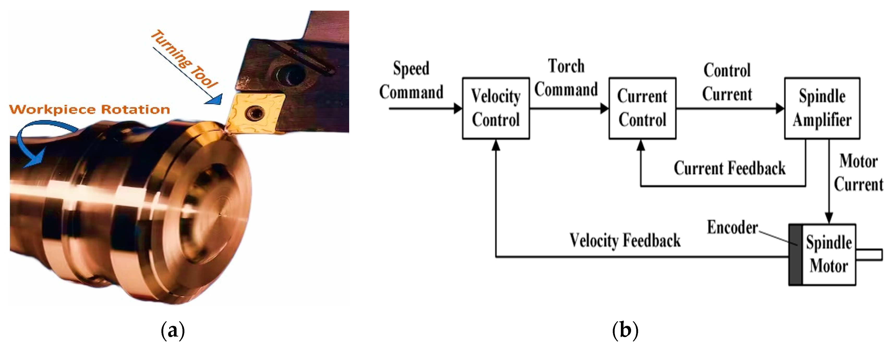
Figure 1. (a) A mechanism in the turning process; (b) The schematic of the spindle control system.
Machines 11 00781 g001
Figure 2. The features from the proposed feature extraction process are used to form our stochastic degradation process of GBM and the prognostics are performed by time series transformer-based prediction.
Machines 11 00781 g002
Figure 3. The shape of the sub-spindle motor current signal from tool 5454. (a) Defining the cutting operation with detail; (b) The shape of each motor current under the cutting process in all three stages.
Machines 11 00781 g003
Figure 4. Removing the carrier signal with the envelope demodulation method.
Machines 11 00781 g004
Figure 5. (a) Reconstructed envelope time motor current signal; (b) The captured central frequencies of MFs corresponding to the odd and even harmonics of the motor current signal for both Tool 5454 and Tool 3636 during one of the experimental runs.
Machines 11 00781 g005
Figure 6. Nine different cutting process features of tool 3636: (a) Demodulated time domain motor with the current signal of metal cutting for tool 3636; (b) Reconstructed envelope feature of the motor current under metal cutting with selected IMFs in the range of tool 3636 harmonics in frequency domain; (c) Proposed reconstructed envelope time domain features of tool 3636.
Machines 11 00781 g006
Figure 7. Four features of the cutting process of tool 5454: (a) Demodulated time domain motor current signal of metal cutting for tool 5454; (b) Reconstructed envelope feature of motor current under metal cutting with selected IMFs in the range of tool 5454 harmonics in the frequency domain; (c) Proposed reconstructed envelope time domain features of tool 5454.
Machines 11 00781 g007
Figure 8. The comparison of odd and even harmonics of THD in different states for two tools. (a) The THD of odd and even harmonics is compared to the healthy state of tool 3636. (b) The comparison of the odd and even harmonics of THD in the wear state of tool 5454.
Machines 11 00781 g008
Figure 9. A comparison was made between the features of the healthy state and wear state for tools (a) 3636 and (b) 5454.
Machines 11 00781 g009
Figure 10. The run-to-wear metal cutting process, focusing on extracted odd and even features. (a) Tool 3636, (b) Tool 5454.
Machines 11 00781 g010
Figure 11. The normalized degradation modeling of historical data using GBM for both tools perfectly show that the time-to-failure could be extracted by the probability of RUL. The utilization of the entire process of odd THD as an input to the degradation models resulted in the generation of random walk paths for historical data. In our analysis, we designated the last 40 percent of the model as the critical region for both Tool 3636 (a) and Tool5454 (b).
Machines 11 00781 g011aMachines 11 00781 g011b
Figure 12. The normalized degradation modeling for even THD demonstrates that the degradation path follows a progressive pattern; however, it does not consistently exceed the critical threshold compared to the proposed features. The attempted degradation modeling of the proposed Even-Features on Tool 3636 (a) and Tool 5454 (b) for GBM has not been successful.
Machines 11 00781 g012
Figure 13. (a) TST values over epochs during the training process., (b) Training process mean the absolute error for the last 10 epochs.
Machines 11 00781 g013
Figure 14. Sub-figures (ac) display the real-time prognostic results of Table 2 for the validation set of Tool 3636, considering three different dates corresponding to three different dates when the tools were changed due to severe wear. The TST method, in conjunction with GBM, successfully predicted unsupervised validation by forecasting the step-ahead degradation path up to the wear point.
Machines 11 00781 g014aMachines 11 00781 g014b
Figure 15. Sub-figures (ac) display the real-time prognostic results of Table 2 for the validation set of Tool 5454 considering three different dates with a broken tool on 30 January 2019. The TST method, in conjunction with GBM, successfully predicted the unsupervised validation by forecasting the step-ahead degradation path up to the wear point.
Machines 11 00781 g015
Table 1. Steps to complete the VMD algorithm.
Variational Mode Decomposition Algorithm
Step 1. Initialization:
m o d e ^ k 0 , ω k 0 ,   λ 0 ^   a n d   n = 0  
Step 2. Updating m o d e k and ω k according to Equation (5)
Step 3. Update λ , for all positive ω :
       λ k n + 1 ω = λ ^   n ω + τ f ^ ω k m o d e i ^ ω ,
τ is the Lagrangian multiplier
Step 4. Convergence check:
condition:   k m o d e k n + 1 m o d e k n 2 2 m o d e k n 2 2 < ε
  • If the convergence condition is met, suspend the iteration.
  • Otherwise, return to step 2.
Table 2. Remaining useful cycles of Tool 5454 and Tool 3636 in real-time prediction.
Tool NumberFailure TypeDateRUL (Cycle = 2 min)Predicted Cycles to Wear (Cycle = 2 min)
Figure 14a3636Severe Wear15 November 20182826
Figure 14b3636Severe Wear16 November 20187944
Figure 14c3636Severe Wear19 November 20183421
Figure 15a5454Severe Wear16 November 20184439
Figure 15b5454Severe Wear19 November 2018126146
Figure 15c5454Broken30 January 20194640
Disclaimer/Publisher’s Note: The statements, opinions and data contained in all publications are solely those of the individual author(s) and contributor(s) and not of MDPI and/or the editor(s). MDPI and/or the editor(s) disclaim responsibility for any injury to people or property resulting from any ideas, methods, instructions or products referred to in the content.