Abstract
In the present research, AISI P20 mold steel was processed using the milling process. The machining parameters considered in the present work were speed, depth of cut (DoC), and feed (F). The experiments were designed according to an L27 orthogonal array; therefore, a total of 27 experiments were conducted with different settings of machining parameters. The response parameters investigated in the present work were material removal rate (MRR), surface roughness (Ra, Rt, and Rz), power consumption (PC), and temperature (Temp). The machine learning (ML) approach was implemented for the prediction of response parameters, and the corresponding error percentage was investigated between experimental values and predicted values (using the ML approach). The technique for order of preference by similarity to ideal solution (TOPSIS) approach was used to normalize all response parameters and convert them into a single performance index (Pi). An analysis of variance (ANOVA) was conducted using the design of experiments, and the optimized setting of machining parameters was investigated. The optimized settings suggested by the integrated ML–TOPSIS approach were as follows: speed, 150 m/min; DoC, 1 mm; F, 0.06 mm/tooth. The confirmation results using these parameters suggested a close agreement and confirmed the suitability of the proposed approach in the parametric evaluation of a milling machine while processing P20 mold steel. It was found that the maximum percentage error between the predicted and experimental values using the proposed approach was 3.43%.
1. Introduction
AISI P20 mold steel is a commonly used steel with a variety of applications. This steel with low alloying elements exhibits good strength and toughness behavior. One of its common applications is plastic injection machinery, where it is used for mold cavities, as well as for casting dies in the casting of zinc. As mentioned by the AISI (American Iron and Steel Organization) procedure for evaluating alloy steel, AISI 316 stainless steel (AISI 316 SS) is most generally used, followed by AISI 304 [1,2]. Numerous industrial sectors, including the medical, aerospace, and automotive industries, make extensive use of stainless-steel alloys [3,4]. However, there are numerous obstacles and difficulties associated with stainless-steel machining [5,6], due to its high strength, low thermal conductivity, and tendency to harden [7]. Stainless-steel alloys are known as very hard materials which are challenging to machine, resulting in an inferior surface finish, sporadic wear, and breakdown of the tool [8]. The work’s surface integrity is compromised, and tool wear is increased when a build-up edge is present. Stainless-steel face milling can resolve these issues. In modern industrial manufacturing, milling is a common and effective machining operation for the fabrication of numerous mechanical parts such as flat surfaces, grooves, threads, and other complex geometric shapes [9]. Cutting tools are crucial parts of the machine milling operation, and they wear out over time. As a result, their conditions change over their effective lifetimes. Machining is an imperative material removal procedure in manufacturing that attracts huge consideration due to its direct link with time and money. A method for monitoring tool wear is, thus, essential as machining applications expand.
Micromachining is acquiring significance because of the increasing need for different miniature parts in biomedical and microelectronics applications [10,11]. One such approach, micro-milling, is a highly favored miniature manufacture process due to its adaptability in assembling three-dimensional complex shapes with a higher material removal rate and precision [12]. One of the significant uses of the micro-milling process is the manufacturing of micro-injection molds, which are exceptionally fundamental for the assembly of polymer micro-components. A huge variety of die steels can be explicitly utilized for mold making. P20 steel is one example. It is a low-carbon steel made by hardening in a carburizing medium. Because of its inherent toughness and hardness, it is especially good for injection molding.
Many experimental and analytical studies have been performed to investigate the minimum uncut chip thickness (MUCT) and the micro-cutting force at a small depth of cut while considering influencing parameters such as the tool edge radius and the coefficient of friction [13,14,15]. The MUCT in micro-milling is crucial when choosing the feed rate and implementing the chip formation process. In a previous study, micro-milling of P20 die steel was carried out to examine the impact of the size and MUCT on chip morphology and tool wear patterns [16]. Twisted and helical chips were acquired at feed rates greater than the MUCT, while chips with erratic shapes were obtained at feed rates beneath the MUCT. At the chip’s free surface, lamellar structures with both an inclined and a vertical orientation were noticed. At feed values below the MUCT, edge-rounding, coating delamination, and built-up edge formation were observed as a result of the size effect.
A micro-machining tool has a low stiffness value, making it susceptible to deflection, which in turn causes chatter, tool wear, severe tool breakage, and inferior surface generation [17]. These issues become even more serious when hard materials are micro-milled. A cutting tool’s hard coating, which has a lower coefficient of friction, can be used to overcome these obstacles and improve tooling performance by reducing tool wear and tool breakage [18]. An insightful model was developed to predict the cutting force and dynamic strength for micro-machining using a TiAlN-coated tool. The model was developed by calculating the modified limiting angle values due to tool failure and incorporating the extracted force coefficients from a thermomechanical-based finite element method (FEM) simulation. The authors also combined the effects of tool failure, minimum chip thickness (MCT), ploughed area, limiting angle values, and elastic recovery, and they developed mechanistic models to predict cutting forces in both shearing- and ploughing-dominant regions using cutting coefficients obtained through FEM simulation while taking the coating material effects into account. The prediction results were compared for coated and uncoated tools, and it was reported that the model provided a viable solution [19,20,21].
Previous research has detailed the machining of different type of steels and parametric optimization [22,23,24,25,26,27,28]. However, it is evident from the literature that limited work has been published on the milling of P20 mold steel. Furthermore, it can be found from the literature that no or limited research has been published on the integrated approach of machine learning and TOPSIS. Therefore, in the current study, an integrated approach of ML–TOSPSIS was used to optimize the milling of P20 mold steel by varying speed, DoC, and feed. The objectives of the present research are as follows:
- To predict the response variables using the ML approach, considering the speed, depth of cut, and feed as independent variables, and Ra, Rt, Rz, PC, temperature, and MRR as dependent variables.
- To investigate the percentage error in the experimental values and predicted values.
- To determine the variation in response variables (i.e., Ra, Rt, Rz, PC, temperature, and MRR) with the input process variables.
- To convert all response variables into a single response (Pi), and to rank all solutions using TOPSIS.
- To validate the predicted solutions after performing confirmation experiments using the suggested optimized parameters.
2. Materials and Methods
There are a large number of applications for AISI P20 mold steel. The attractive mechanical properties of mold steels made them a strategic material fitting civilian and military application needs. Their machining quality is of primary importance to fully benefit from this type of material. In this work, we study the optimum cutting conditions (speed, feed, and depth of cut) to find the minimum surface roughness, cutting temperature, and power consumption obtained with dry conditions. The AISI P20 mold steel used in this study is defined chemically and mechanically in Table 1 and Table 2 below. The AISI P20 steel was in tempered condition to relieve the residual stresses. The chemical and mechanical characteristics were investigated in the material research laboratory.

Table 1.
AISI P20 mold steel chemical composition (percent by mass).
Table 2.
AISI P20 mold steel mechanical properties.
Optical microscope (OM) manufactured by Olympus, model: BX51-M, was used for the metallographic investigations. The steel P20 has medium C content and alloying elements, as shown in Table 1. The steel is usually provided in tempered conditions. The produced microstructure is tempered martensite. The martensite is a hard metastable structure with a body-centered tetragonal (BCT) crystal structure. It is formed in steels when quenching/cooling from the austenite range, in which carbon atoms do not have time to diffuse out of the crystal structure in sufficient enough quantities to form cementite (Fe3C). Figure 1 shows the microstructure of tempered martensite, which includes short martensite laths and carbides (dark phase) within the ferrite matrix (white phase). The arrows represent the carbide particles present in the material.
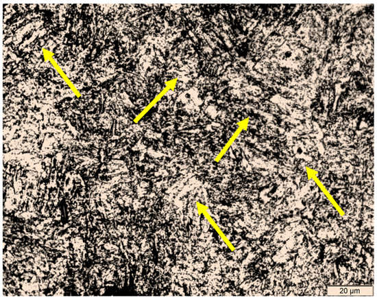
Figure 1.
Tempered martensite microstructure.
Test specimens of rectangular surface area 100 × 40 mm and 25 mm height were used in all trial tests. The samples were milled using an Emco Mill C40 standard milling machine with vertical milling direction from Emco of Salzburg, Austria. The power of the machine shaft is 13 KW. The revolution capacity spans the range of 10–5000 RPM. The steeples range of the counter has a feed rate range of 10–2000 mm/min. The face milling cutter and inserts were manufactured by Sandvik (Sandvik, Stockholm, Sweden). The holder is a milling cutter with code: R245-063Q22-12M. The insert code is: R245-12T3M-PM 4330 (corner radius: 1.5 mm; insert rake angle: 15°; major cutting-edge angle: 45°; coating: TiCN + Al2O3 + TiN). There are five inserts with a 63 mm cutter diameter. The cutter is designed for high-quality surface finishes at efficient material removal rates. It is typically employed for the removal of various metals from steel alloys to titanium alloys.
Figure 2a represents the workpiece used in the current work, while Figure 2b shows the carbide tools used to machine P20 mold steel. Figure 3 is a photograph of the experimental setup of the milling process of samples with data recording tools.
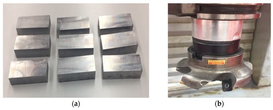
Figure 2.
(a) Work-piece used in current research and (b) carbide tool used to machine P20 steel.
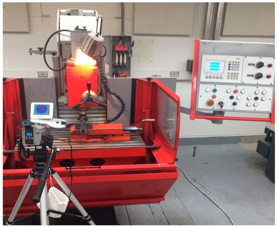
Figure 3.
Experimental setup for milling of AISI P20 samples with thermal camera.
The test plan contains a total of 27 experiments. These cover the main milling variables, which are the surface speed (V) measured in m/min, the axial depth of cut () measured in mm per tooth, and the width of cut and the feed per tooth (F), both of which are measured in mm. These process parameters’ range and levels are selected after performing preliminary experiments in different settings. The speed is assigned to 50, 100 and 150 m/min, the depth of cut is assigned to 0.5, 0.75 and 1.0 mm, and the feed per tooth is assigned the values 0.02, 0.04 and 0.06 mm. The fourth one, which is the width of the cut, is fixed to 40 mm. The total combination is 27 independent cases. Moreover, the sample length is fixed at 100 mm for all cases. All tests are performed in dry conditions two times, and the average of two is considered for calculation purposes to maintain statistical accuracy.
The surface roughness tester type for evaluation of surface roughness grade is Tesa-Rougossurf-90G of Tesa company, Bugnon, Switzerland. The device is shown in Figure 4, where parameters and are evaluated for all experiments that were recorded. The parameters selected for measuring surface roughness are: cut-off length: 0.8 mm; measurement surface: plain; measurement speed: 1 mm/s; cut-off number: 19; gauge type: skid.
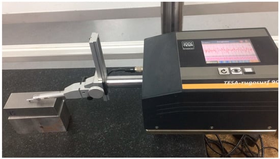
Figure 4.
Setup for evaluating surface roughness quality of milled samples.
Measurement of power consumption during milling runs is achieved by two power meters (Tactix 403057, Beijing, China). The two power meters are attached to the milling machine power supply to measure the voltage and current during the face milling process. Consumed power is evaluated by measurement of the current (I) in one line and the voltage difference (V) between, through a balanced three-phase load-cutting machine. Figure 5 illustrates the setup for power measurement. For each milling run, three sets of readings are recorded from which the average is evaluated so that the power (P) is calculated according to Equation (1), and (ø) is the power factor for a three-phase machine.
Total power = Voltage × Current × √3 COS ø = Wa

Figure 5.
Setup for power consumption measurement.
A ThermoPro-TP8 thermal camera from Guide company, Wuhan, China, is utilized to record the thermal data during milling runs. Figure 6 shows the thermal camera set-up, and Table 3 gives its specific details.
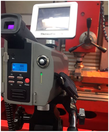
Figure 6.
ThermoPro-TP8 thermal camera for thermal imaging.
Table 3.
Data of ThermoPro-TP8 thermal camera [29].
The camera must be correctly calibrated to achieve stable and focused thermal images. Whether using the camera′s auto-calibration feature or manual calibration, the focus of the image must be ensured by giving enough time for the focus before starting the process. This way, appropriate sensitivity is ensured and the camera is focused on the workpiece during the milling to reflect the temperature.
Figure 7 shows the camera during milling with a focus on the workpiece with an appropriate distance, which must be fed to the camera for the proper reported temperature value. The set value of the material emissivity coefficient is based on the recommended values table in the camera manual. In general, emissivity is a function of the target surface quality (roughness), the heat intensity, the target material type, the wavelength and the angle of attack.
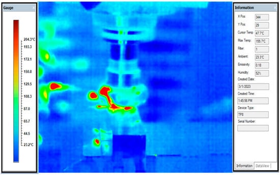
Figure 7.
ThermoPro-TP8 recording of temperature at surface speed = 100 m/min, depth of cut = 0.50 mm and feed rate = 0.04 mm/tooth.
3. Methodology
The methodology adopted in the present research for optimizing process parameters while machining P20 steel is presented in Figure 8. In the first step of the process, the parameters are investigated for the working range, and in the working range the experimental layout is developed. A machine learning approach is implemented in the next step to find the predicted solution. The ML approach’s perspective is to find the solutions out of the search space for the possible hypothesis and predict the best solution.
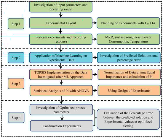
Figure 8.
Process procedure adopted in the present research.
In the next step, TOPSIS is applied to the predicted solution suggested by the ML approach. Hwang and Yoon [30] developed the TOPSIS technique in 1981. This technique helps to identify the best choice after comparing it with the ideal solution. The identified solution is nearer to the positive ideal solution while far away from a negative ideal solution. The positive ideal solution is selected for maximizing the profit and minimizing the cost; however, the negative ideal solution is selected to maximize the cost criteria and minimize the profit criteria. This technique is extensively used to solve the MCDM problems associated with the manufacturing sectors and is supported by numerous researchers. This method is associated with two different types of solutions: the first type is negative (or worst), and the second type is positive (or best). The best solution is predicted from the alternative solutions.
The TOPSIS method starts with developing a decision matrix (known as a normal decision matrix) depending on the nature of the response variable. This matrix contains the details for the alternative and the problem criteria. The weights are decided according to the importance given to each response. After that, the weighted decision matrix is evaluated by multiplying the normal decision matrix by the weight given to each response. Two categories of solutions are calculated: worst-type solutions and best-type solutions. These two solutions are further used to calculate the separation distance for each criterion. In the final step, the performance index is calculated, and the rank of each experimental setting is given. The confirmation experiments were conducted in the fourth step, and the percentage error was investigated between the predicted and experimental values.
4. Results and Discussion
The experimental layout of input process variables shows the L27 orthogonal array and the values of responses corresponding to the experimental layout (Table 4).
Table 4.
Experimental layout and corresponding results.
4.1. Variation of the Responses with the Input Variables
The statistical summary of the research is given in the appendix Table A1, Table A2, Table A3, Table A4, Table A5, Table A6 and Appendix A, where the ANOVA for all the responses is provided. It is clear from the ANOVA that more than 98% variability can be explained from the present model due to significant and non-significant terms (R2) and significant terms (R2 adj). Figure 9 depicts the variation of the response variables concerning the input control variable. It is evident that with the increase in speed value, the Ra, Rt and Rz value decreases, i.e., surface finish increases. The main reason is the removal of debris from the material surface at a faster speed. Due to this, the craters from the surface are removed efficiently.
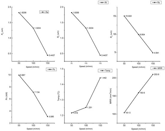
Figure 9.
Variation of response parameters with the speed.
The Ra is the average surface roughness of the machined surface. The Rz is the mean of five consecutive peaks and valleys, while Rt is the difference between the highest peak and deepest valley. Therefore, every type of surface roughness depends upon the crater size. An increase in the speed value decreases the crater size and hence decreases the Ra, Rt and Rz (Figure 9). With the increase in speed value from 50 m/min to 150 m/min, the PC decreases from 9.987 kW to 3.085 kW. This decrement in energy consumption is the decrease in crater size, which reduces the forces required to machine the material and hence the PC value. The temperature value increases from 1216 °C to 1442 °C with an increase in speed from 50 m/min to 150 m/min. The probable reason for this increment in temperature is the high speed. With the increase in speed, the temperature dissipation from the chip decreases, which increases the temperature. Figure 9 shows that with the increase in speed value, the MRR enhances from 161.5 mm3/min to 203.9 mm3/min. The probable reason for the increase in MRR with the speed value is the higher material removal in the given time.
Figure 10 represents the variation of output parameters with respect to the DoC. Figure 10 shows that with the increase in DoC value from 0.5 mm to 0.75 mm, the surface roughness values (Ra, Rt and Rz) increase. After that, DoC increases from 0.75 mm to 1 mm and the SR value (Ra, Rt and Rz) also decreases. With the increase in DoC value, the crater size increases, which increases the SR (Ra, Rt and Rz) values. Once the DoC value further increases, the SR value decreases. The probable reason for this decrement may be the dynamic behavior (low vibration) of the chip load at high value of DoC. These results are inline with the previous published results [31]. The similar pattern is observed for PC with the increase in DoC. The reason behind this pattern is the energy consumption increases initially with the DoC increment from 0.5 to 0.75 mm. Further increases in DoC decrease the vibrations and hence decrease the energy consumption. Figure 10 depicts that an increase in DoC value increases the temperature. The reason for this is the large amount of resistance, which increases the cutting temperature from 1235 °C to 1379 °C. The MRR value amplifies from 155.4 mm3/min to 204.2 mm3/min with the increase in DoC from 0.5 mm to 1 mm. The reason behind this enlargement is the large amount of material removal with the increase in DoC.
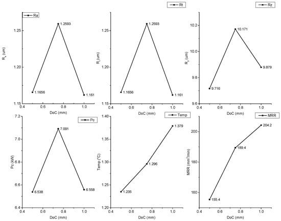
Figure 10.
Variation of response parameters with the DoC.
Figure 11 presents the variation of response variables with respect to the ‘F’ value. It is clear from Figure 11 that with the increase in F value (from 0.02 mm/tooth to 0.06 mm/tooth), the SR values (Ra, Rt and Rz) increase. The increase in F value increases the crater size, which increases the surface roughness values (Ra, Rt and Rz). Figure 11 reveals that with the increase in F value, the PC increases from 6.017 kW to 7.363 kW. The main reason for this PC enhancement is the increase in cutting forces with the increase in F value from 0.02 to 0.06 mm/tooth. To overcome the cutting resistance, more energy is consumed for the cutting operation. Similarly, with the increase in F values, the cutting resistance increases the cutting temperature (from 1239 °C to 1374 °C). Figure 11 also shows the variation of MRR (170.5 mm3/min to 196.5 mm3/min) with the increase in feed rate value.
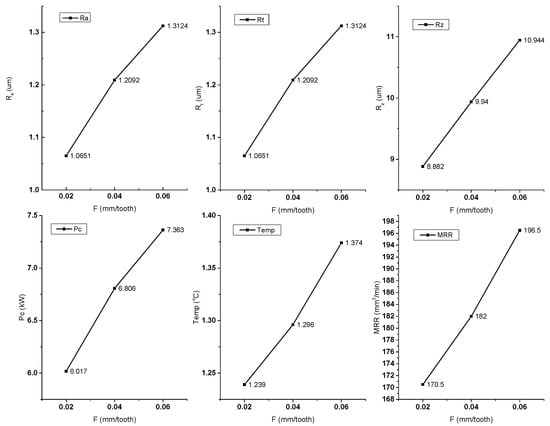
Figure 11.
Variation of response parameters with the feed.
4.2. Correlation Investigation
In this section, correlation coefficients are computed between the input parameters and response variables. The correlation coefficient may be positive or negative. A negative correlation exists if, during observation, one variable increases and the other decreases. The value of correlation is zero if there is no correlation. The value of correlation is positive if both the variables increase or decrease at the same time.
Two different correlation plots are depicted in Figure 12 and Figure 13. In Figure 12, the correlation values are depicted, while in Figure 13 the correlation is represented with the help of colors. It is clear from Figure 12 that the correlation coefficient value for the case of speed vs. Ra, Rt and Rz is negative. The main fact of the negative correlation is the decrement in the response parameters with respect to the counter parameter. Furthermore, the value of PC increases with the increase in temp and MRR value; therefore, both represent positive correlation values (0.860 and 0.924, respectively). Figure 13 depicts the color mapping of the correlation coefficient for input parameters and output response variables. The dark blue color depicts the correlation value equal to 1 and dark brown color shows the correlation value equal to −1.
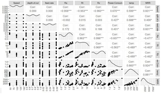
Figure 12.
Correlation coefficient investigation with the machining parameters and response parameters. Each significance level is associated to a symbol: p-values (0, 0.001, 0.01, 0.05) <=> symbols (“***”, “**”, “*”).
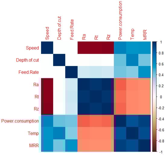
Figure 13.
Color mapping of correlation coefficient.
4.3. Prediction for Solutions
The machine learning approach is used to investigate the response variables. The experimental data obtained after performing experiments were solved using ‘R’. The obtained data are divided into three parts; namely, training data, testing data and validation data. Overall, 70% of data of 27 experiments are used for training and the remining 30% of data are divided into testing (15%) and validation (15%). The experimental results of MRR, Ra, Rt, Rz, PC and temp were put as response parameters against the input parameters (speed, DoC and feed). The predicted solutions are checked against the experimental results.
Figure 14 shows the experimental versus predicted values for different response variables like Ra (Figure 14a), Rz (Figure 14b), Rt (Figure 14c), PC (Figure 14d), temperature (Figure 14e) and MRR (Figure 14f). It is evident from Figure 14 that experimental values are totally superimposed by the predicted values. The variation of all the predicted values are inline with the experimental values. Therefore, the investigation of the response variables while machining P20 steel on CNC milling is successfully predicted by the proposed approach. The predictive equations for all the response variables are provided from Equation (2) to Equation (7).
Ra = 2.551 − 0.01327 × Speed − 0.522 × DoC + 3.58 × F + 0.00155 × Speed × DoC − 0.0415 × Speed × F + 9.02 ×
DoC × F
DoC × F
Rt = 16.48 − 0.0897× Speed + 0.09 × DoC + 91.5 × F + 0.0037 × Speed × DoC − 0.374 × Speed × F − 3.4 × DoC ×
F
F
Rz = 13.23 − 0.0696 × Speed − 2.37 × DoC + 30.9 × F + 0.0118 × Speed× DoC − 0.203 × Speed × F + 30.7 × DoC
× F
× F
PC = 1.352 − 0.00237 × Speed − 0.344 × DoC − 4.57 × F + 0.00413 × Speed × DoC + 0.0383 × Speed × F + 5.50 ×
DoC × F
DoC × F
Temp = 74.6 + 0.195 × Speed + 61.3 × DoC + 244 × F + 0.226 × Speed × DoC + 1.50 × Speed × F + 342 × DoC ×
F
F
MRR = 3000 − 30.00× Speed − 4000 × DoC – 75,000 × F + 40.00 × Speed × DoC + 750.0 × Speed × F + 100,000
× DoC × F
× DoC × F
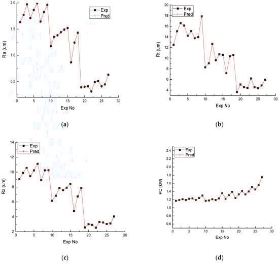
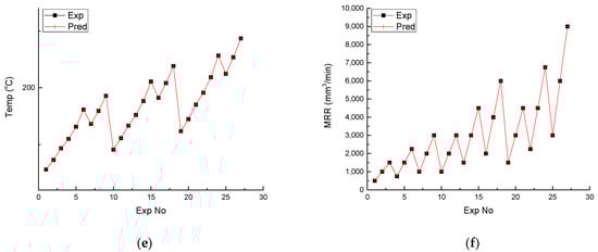
Figure 14.
Experimental versus predicted results for different response parameters. (a) Experimental vs. predicted for Ra; (b) experimental vs. predicted for Rt; (c) experimental vs. predicted for Rz; (d) experimental vs. predicted for PC; (e) experimental vs. predicted for temperature; (f) experimental vs. predicted for MRR.
Figure 15 shows the error percentage plot in the experimental and predicted values of the responses. The error plot reveals that the values of the predicted solution have the close agreement with the experimental values. Error percentage plots of Ra (Figure 15a), Rz (Figure 15b), Rt (Figure 15c), PC (Figure 15d), temperature (Figure 15e) and MRR (Figure 15f) are depicted. It is clear from Figure 15 that the maximum error percentage in the predicted values is ±1%, which signifies the importance of the proposed approach in the present research.

Figure 15.
Percentage error plot for different response parameters. (a) Plot of Ra error %; (b) plot of Rt error %; (c) plot of Rz error %; (d) plot of PC error %; (e) plot of temperature error %; (f) plot of MRR error %. The accuracy percentage of the predicted values after the implementation of ML for each response is shown in Figure 16. It is clear from Figure 16 that the accuracy of the predicted values in each case is greater than 99%, which signifies the importance of the ML approach for the investigation of responses while machining the P20 steel.
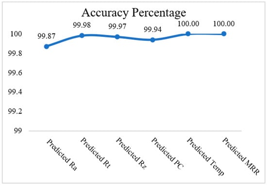
Figure 16.
Accuracy percentage of the predicted values.
4.4. Implementation of TOPSIS on Predicted Values
The response characteristics have different units and magnitude; therefore, it became mandatory to convert them into some comparable values. Thus, the normalization plays a vital role in the optimization process. In the normalization process, the responses are converted into a dimensionless number (0 to 1). Therefore, all the responses from the diverse measurement are converted into a number for ranking purpose in the decision-making issues [29]. This method is suitable for the problems, where an involvement of two of more than two responses exists. The following steps are followed for investigating the performance index:
In the first step, the nature of the response variables is identified. Whether it is larger than the better type or smaller than the better type.
The normalization of the responses are made using Equation (8) and a decision matrix is developed in the second step (Table 5).
Table 5.
Normalized decision matrix of the response variable.
In this step, the weighted normalized value is evaluated using Equation (9). The weights are predicted depending upon the importance of the respective response characteristics. In the present work, all the response characteristics were given equal importance, i.e., 0.17 (Table 6).
Table 6.
Weighted normalized values and performance index.
In the next step, we have alternative positive and negative seperation solutions using Equations (10) and (11).
The performance index is calculated using Equation (12) (Table 6).
It is evident that higher value of Pi is desirable for the overall better performance of the process. It is clear from Figure 17 that the third level of CS (150 m/s), third level of DoC (1 mm) and third level of F (0.06 mm/rev) favor the highest Pi.
Figure 17.
Variation of Pi with respect to input parameters.
Table 7 gives the ANOVA of Pi and shows that the speed, DoC, F and interaction of speed and DoC, speed and F and DoC and F play significant roles in the investigation of Pi due to a p-value less than 0.05. From the F-value, it is clear that ‘speed’ has the maximum contribution, followed by speed and DoC. The values of R2 and adj R2 are also in close agreement, which depicts that the 99.69% variability can be explained due to significant and non-significant parameters, while 98.98% variability is explained with the significant factors only. The empirical model develop for Pi is provided in Equation (13).
Pi = 0.3051 + 0.000578 × Speed − 0.228 × DoC − 6.19 × F + 0.002028 × Speed ×
DoC + 0.04958 × Speed × F + 4.15 × DoC × F
DoC + 0.04958 × Speed × F + 4.15 × DoC × F
Table 7.
Analysis of variance for Pi.
4.5. Confirmation Experiments
The confirmation experiments are conducted to validate the results obtained after the integrated approach of machine learning and TOPSIS. Due to highest value of Pi corresponding to experimental run number 27, the confirmation experiments are conducted on this experimental setting (Speed150DoC1F0.06).
The percentage error between the predicted and experimental values is investigated and it is found that the maximum percentage error observed is 3.43% (Table 8). This signifies the suitability of the proposed approach for the optimization of the process parameters while machining P20 steel.
Table 8.
Predicted, experimental and percentage errors for the confirmation results.
5. Conclusions
The P20 mold steel has different applications in plastic injection machinery where it is used as mold cavities, as casting dies for casting of zinc. The effective use of P20 steel can be made after making the product, which needs the machining to obtain the shape of the product. Therefore, in the current work, P20 mold steel is processed on a milling machine at different settings of speed, DoC and feed to investigate different response parameters like surface roughness, MRR, PC, and temperature. The main conclusions drawn from the current research are as:
The overall accuracy of the predicted solution by the ML-approach is more than 99% for all the response parameters; thus, the proposed approach is successfully implemented for the investigation of solutions while processing P20 mold steel on a milling machine.
The correlation coefficient is minimum, i.e., −0.960, for the case of Rz and speed, which signifies the decrease in the Rz value with respect to speed. However, the maximum correlation (0.996) exists for the case of Rz and Ra, where the value of Rz increases with the increase in Ra value.
The integrated approach of ML-TOPSIS suggests that the maximum predicted Pi is 0.7754 corresponding to the optimized setting, i.e., speed: 150 m/min; DoC: 1 mm and F: 0.06 mm/tooth. The proposed model predicts the solutions nearby the experimental value with a maximum percentage error of 3.43%.
The investigated outcomes from the research shows the benefit of the proposed soft computing technique to find out the optimized machining conditions with balanced performance of the response characteristics.
The proposed technique can be implemented for the investigation of other response characteristics, and to analyze and optimize the process parameters for other types of materials used in different industries. In the future, this methodology can also be used for other machining methods (namely conventional as well as non-conventional). The effect of change of tool materials on response characteristics can also be considered in upcoming research. The soft computing technique can be used for optimizing the process parameters via an online method, and tool condition monitoring may be another perspective via the proposed approach.
Author Contributions
A.T.A., N.S. and Z.A.A.: Investigation, conceptualization, methodology, data curation, validation, visualization; A.E., I.F. and A.S.: investigation, writing—original draft, writing, conceptualization, supervision, project administration: Review and editing; A.T.A.: funding acquisition. All authors have read and agreed to the published version of the manuscript.
Funding
Grant: (IFKSUOR3–040-3).
Data Availability Statement
Not applicable.
Acknowledgments
The authors extend their appreciation to the Deputyship for Research and Innovation, Ministry of Education in Saudi Arabia for funding this research work through the project no. (IFKSUOR3–040-3).
Conflicts of Interest
The authors declare that they have no known competing financial interests or personal relationships that could have appeared to influence the work reported in this paper.
Appendix A
Table A1.
ANOVA for Ra Means.
Table A1.
ANOVA for Ra Means.
| Source | DF | SS | MS | F | P |
|---|---|---|---|---|---|
| Speed | 2 | 8.75257 | 4.37628 | 644.10 | 0.000 |
| DoC | 2 | 0.05529 | 0.02764 | 4.07 | 0.060 |
| F | 2 | 0.27849 | 0.13925 | 20.49 | 0.001 |
| Speed × DoC | 4 | 0.10533 | 0.02633 | 3.88 | 0.049 |
| Speed × F | 4 | 0.02804 | 0.00701 | 1.03 | 0.447 |
| DoC × F | 4 | 0.03312 | 0.00828 | 1.22 | 0.375 |
| Residual Error | 8 | 0.05436 | 0.00679 | ||
| Total | 26 | 9.30719 | R2: 99.42%; R2 (adj): 98.10% | ||
Table A2.
ANOVA for Rt Means.
Table A2.
ANOVA for Rt Means.
| Source | DF | SS | MS | F | P |
|---|---|---|---|---|---|
| Speed | 2 | 466.493 | 233.246 | 206.57 | 0.000 |
| DoC | 2 | 0.955 | 0.478 | 0.42 | 0.669 |
| F | 2 | 19.134 | 9.567 | 8.47 | 0.011 |
| Speed × DoC | 4 | 1.592 | 0.398 | 0.35 | 0.835 |
| Speed × F | 4 | 6.404 | 1.601 | 1.42 | 0.312 |
| DoC × F | 4 | 9.592 | 2.398 | 2.12 | 0.169 |
| Residual Error | 8 | 9.033 | 1.129 | ||
| Total | 26 | 513.204 | R2: 98.24%; R2 (adj): 94.28% | ||
Table A3.
ANOVA for Rz Means.
Table A3.
ANOVA for Rz Means.
| Source | DF | SS | MS | F | P |
|---|---|---|---|---|---|
| Speed | 2 | 215.381 | 107.690 | 561.08 | 0.000 |
| DoC | 2 | 1.776 | 0.888 | 4.63 | 0.046 |
| F | 2 | 8.239 | 4.120 | 21.46 | 0.001 |
| Speed × DoC | 4 | 2.681 | 0.670 | 3.49 | 0.062 |
| Speed × F | 4 | 1.154 | 0.288 | 1.50 | 0.289 |
| DoC × F | 4 | 0.492 | 0.123 | 0.64 | 0.649 |
| Residual Error | 8 | 1.535 | 0.192 | ||
| Total | 26 | 231.257 | R2: 99.34%; R2 (adj): 97.84% | ||
Table A4.
ANOVA for PC Means.
Table A4.
ANOVA for PC Means.
| Source | DF | SS | MS | F | P |
|---|---|---|---|---|---|
| Speed | 2 | 0.267496 | 0.133748 | 227.84 | 0.000 |
| DoC | 2 | 0.094630 | 0.047315 | 80.60 | 0.000 |
| F | 2 | 0.083430 | 0.041715 | 71.06 | 0.000 |
| Speed × DoC | 4 | 0.036770 | 0.009193 | 15.66 | 0.001 |
| Speed × F | 4 | 0.018304 | 0.004576 | 7.79 | 0.007 |
| DoC × F | 4 | 0.009437 | 0.002359 | 4.02 | 0.045 |
| Residual Error | 8 | 0.004696 | 0.000587 | ||
| Total | 26 | 0.514763 | R2: 99.09%; R2 (adj): 97.03% | ||
Table A5.
ANOVA for Temp Means.
Table A5.
ANOVA for Temp Means.
| Source | DF | SS | MS | F | P |
|---|---|---|---|---|---|
| Speed | 2 | 8103.0 | 4051.51 | 45,109.62 | 0.000 |
| DoC | 2 | 11,257.1 | 5628.56 | 62,668.53 | 0.000 |
| F | 2 | 3054.1 | 1527.07 | 17,002.41 | 0.000 |
| Speed × DoC | 4 | 100.7 | 25.17 | 280.27 | 0.000 |
| Speed × F | 4 | 27.2 | 6.79 | 75.62 | 0.000 |
| DoC × F | 4 | 60.8 | 15.20 | 169.24 | 0.000 |
| Residual Error | 8 | 0.7 | 0.09 | ||
| Total | 26 | 22,603.7 | R2: 99.09%; R2 (adj): 97.03% | ||
Table A6.
ANOVA for MRR Means.
Table A6.
ANOVA for MRR Means.
| Source | DF | SS | MS | F | P |
|---|---|---|---|---|---|
| Speed | 2 | 40,500,000 | 20,250,000 | 324.00 | 0.000 |
| DoC | 2 | 18,000,000 | 9,000,000 | 144.00 | 0.000 |
| F | 2 | 40,500,000 | 20,250,000 | 324.00 | 0.000 |
| Speed × DoC | 4 | 3,000,000 | 750,000 | 12.00 | 0.002 |
| Speed × F | 4 | 6,750,000 | 1,687,500 | 27.00 | 0.000 |
| DoC × F | 4 | 3,000,000 | 750,000 | 12.00 | 0.002 |
| Residual Error | 8 | 500,000 | 62,500 | ||
| Total | 26 | 112,250,000 | R2: 99.55%; R2 (adj): 98.55% | ||
References
- Jabbar Hassan, A.; Boukharouba, T.; Miroud, D.; Titouche, N.; Ramtani, S. Experimental Investigation of Friction Pressure Influence on the Characterizations of Friction Welding Joint for AISI 316. Int. J. Eng. 2020, 33, 2514–2520. [Google Scholar]
- Makwana, A.V.; Banker, K.S. An Experimental Investigation on AISI 316 Stainless Steel for Tool Profile Change in Die Sinking EDM Using DOE. Sch. J. Eng. Technol. 2015, 3, 447–462. [Google Scholar]
- Selembo, P.A.; Merrill, M.D.; Logan, B.E. The Use of Stainless Steel and Nickel Alloys as Low-Cost Cathodes in Microbial Electrolysis Cells. J. Power Sources 2009, 190, 271–278. [Google Scholar] [CrossRef]
- Zhang, E.; Zhao, X.; Hu, J.; Wang, R.; Fu, S.; Qin, G. Antibacterial Metals and Alloys for Potential Biomedical Implants. Bioact. Mater. 2021, 6, 2569–2612. [Google Scholar] [CrossRef] [PubMed]
- Goindi, G.S.; Sarkar, P. Dry Machining: A Step towards Sustainable Machining–Challenges and Future Directions. J. Clean. Prod. 2017, 165, 1557–1571. [Google Scholar] [CrossRef]
- Sankaranarayanan, R.; Krolczyk, G.M. A Comprehensive Review on Research Developments of Vegetable-Oil Based Cutting Fluids for Sustainable Machining Challenges. J. Manuf. Process. 2021, 67, 286–313. [Google Scholar]
- Gardner, L.; Insausti, A.; Ng, K.T.; Ashraf, M. Elevated Temperature Material Properties of Stainless Steel Alloys. J. Constr. Steel Res. 2010, 66, 634–647. [Google Scholar] [CrossRef]
- Maloy, S.A.; James, M.R.; Willcutt, G.; Sommer, W.F.; Sokolov, M.; Snead, L.L.; Hamilton, M.L.; Garner, F. The Mechanical Properties of 316L/304L Stainless Steels, Alloy 718 and Mod 9Cr–1Mo after Irradiation in a Spallation Environment. J. Nucl. Mater. 2001, 296, 119–128. [Google Scholar] [CrossRef]
- Sarıkaya, M.; Gupta, M.K.; Tomaz, I.; Pimenov, D.Y.; Kuntoğlu, M.; Khanna, N.; Yıldırım, Ç.V.; Krolczyk, G.M. A State-of-the-Art Review on Tool Wear and Surface Integrity Characteristics in Machining of Superalloys. CIRP J. Manuf. Sci. Technol. 2021, 35, 624–658. [Google Scholar] [CrossRef]
- Rizvi, N.H. Femtosecond Laser Micromachining: Current Status and Applications. Riken Rev. 2003, 1, 107–112. [Google Scholar]
- Miller, P.R.; Aggarwal, R.; Doraiswamy, A.; Lin, Y.J.; Lee, Y.-S.; Narayan, R.J. Laser Micromachining for Biomedical Applications. Jom 2009, 61, 35–40. [Google Scholar] [CrossRef]
- Baig, A.; Jaffery, S.H.I.; Khan, M.A.; Alruqi, M. Statistical Analysis of Surface Roughness, Burr Formation and Tool Wear in High Speed Micro Milling of Inconel 600 Alloy under Cryogenic, Wet and Dry Conditions. Micromachines 2022, 14, 13. [Google Scholar] [CrossRef]
- Connolly, R.; Rubenstein, C. The Mechanics of Continuous Chip Formation in Orthogonal Cutting. Int. J. Mach. tool Des. Res. 1968, 8, 159–187. [Google Scholar] [CrossRef]
- Liu, X.; DeVor, R.E.; Kapoor, S.G. An Analytical Model for the Prediction of Minimum Chip Thickness in Micromachining. J. Manuf. Sci. Eng. 2006, 128, 474–481. [Google Scholar] [CrossRef]
- Yuan, Z.J.; Zhou, M.; Dong, S. Effect of Diamond Tool Sharpness on Minimum Cutting Thickness and Cutting Surface Integrity in Ultraprecision Machining. J. Mater. Process. Technol. 1996, 62, 327–330. [Google Scholar] [CrossRef]
- Sahoo, P.; Patra, K.; Szalay, T.; Dyakonov, A.A. Determination of Minimum Uncut Chip Thickness and Size Effects in Micro-Milling of P-20 Die Steel Using Surface Quality and Process Signal Parameters. Int. J. Adv. Manuf. Technol. 2020, 106, 4675–4691. [Google Scholar] [CrossRef]
- Bolar, G.; Das, A.; Joshi, S.N. Measurement and Analysis of Cutting Force and Product Surface Quality during End-Milling of Thin-Wall Components. Measurement 2018, 121, 190–204. [Google Scholar] [CrossRef]
- Sahoo, P.; Patra, K.; Singh, V.K.; Gupta, M.K.; Song, Q.; Mia, M.; Pimenov, D.Y. Influences of TiAlN Coating and Limiting Angles of Flutes on Prediction of Cutting Forces and Dynamic Stability in Micro Milling of Die Steel (P-20). J. Mater. Process. Technol. 2020, 278, 116500. [Google Scholar] [CrossRef]
- Padhan, S.; Wagri, N.K.; Dash, L.; Das, A.; Das, S.R.; Rafighi, M.; Sharma, P. Investigation on Surface Integrity in Hard Turning of AISI 4140 Steel with SPPP-AlTiSiN Coated Carbide Insert under Nano-MQL. Lubricants 2023, 11, 49. [Google Scholar] [CrossRef]
- Rafighi, M.; Özdemir, M.; Şahinoğlu, A.; Kumar, R.; Das, S.R. Experimental Assessment and Topsis Optimization of Cutting Force, Surface Roughness, and Sound Intensity in Hard Turning of Aisi 52100 Steel. Surf. Rev. Lett. 2022, 29, 2250150. [Google Scholar] [CrossRef]
- Özdemir, M.; Rafighi, M.; Al Awadh, M. Comparative Evaluation of Coated Carbide and CBN Inserts Performance in Dry Hard-Turning of AISI 4140 Steel Using Taguchi-Based Grey Relation Analysis. Coatings 2023, 13, 979. [Google Scholar] [CrossRef]
- Abbas, A.T.; Sharma, N.; Alsuhaibani, Z.A.; Sharma, V.S.; Soliman, M.S.; Sharma, R.C. Processing of Al/SiC/Gr Hybrid Composite on EDM by Different Electrode Materials Using RSM-COPRAS Approach. Metals 2023, 13, 1125. [Google Scholar] [CrossRef]
- Gaudêncio, J.H.D.; Correa, J.E.; de Carvalho Paes, V.; da Silva Campos, P.H.; Turrioni, J.B.; de Paiva, A.P. Hybrid Multiobjective Optimization Algorithm Based on Multivariate Mean Square Error and Fuzzy Decision Maker. Appl. Soft Comput. 2019, 82, 105586. [Google Scholar] [CrossRef]
- Gupta, P.; Singh, B. Local Mean Decomposition and Artificial Neural Network Approach to Mitigate Tool Chatter and Improve Material Removal Rate in Turning Operation. Appl. Soft Comput. 2020, 96, 106714. [Google Scholar] [CrossRef]
- Hegab, H.; Salem, A.; Rahnamayan, S.; Kishawy, H.A. Analysis, Modeling, and Multi-Objective Optimization of Machining Inconel 718 with Nano-Additives Based Minimum Quantity Coolant. Appl. Soft Comput. 2021, 108, 107416. [Google Scholar] [CrossRef]
- Bohat, M.; Sharma, N. Investigation of parameters and morphology of coated WC tool while machining X-750 using NSGA-II. Eng. Res Express 2023, 5, 25052. [Google Scholar] [CrossRef]
- Gupta, M.K.; Sood, P.K.; Singh, G.; Sharma, V.S. Investigations of Performance Parameters in NFMQL Assisted Turning of Titanium Alloy Using TOPSIS and Particle Swarm Optimisation Method. Int. J. Mater. Prod. Technol. 2018, 57, 299–321. [Google Scholar] [CrossRef]
- Sharma, N.; Gupta, R.D.; Khanna, R.; Sharma, R.C.; Sharma, Y.K. Machining of Ti-6Al-4V biomedical alloy by WEDM: Investigation and optimization of MRR and Rz using grey-harmony search. World J. Eng. 2023, 20, 221–234. [Google Scholar] [CrossRef]
- El Rayes, M.M.; Abbas, A.T.; Al-Abduljabbar, A.A.; Ragab, A.E.; Benyahia, F.; Elkaseer, A. Investigation and Statistical Analysis for Optimizing Surface Roughness, Cutting Forces, Temperature, and Productivity in Turning Grey Cast Iron. Metals. 2023, 13, 1098. [Google Scholar] [CrossRef]
- Hwang, C.-L.; Yoon, K.; Hwang, C.-L.; Yoon, K. Methods for Multiple Attribute Decision Making. Mult. Attrib. Decis. Mak. Methods Appl. A State Art Surv. 1981, 186, 58–191. [Google Scholar]
- Tsao, T.-C.; McCarthy, M.W.; Kapoor, S.G. A New Approach to Stability Analysis of Variable Speed Machining Systems. Int. J. Mach. Tools Manuf. 1993, 33, 791–808. [Google Scholar] [CrossRef]
Disclaimer/Publisher’s Note: The statements, opinions and data contained in all publications are solely those of the individual author(s) and contributor(s) and not of MDPI and/or the editor(s). MDPI and/or the editor(s) disclaim responsibility for any injury to people or property resulting from any ideas, methods, instructions or products referred to in the content. |
© 2023 by the authors. Licensee MDPI, Basel, Switzerland. This article is an open access article distributed under the terms and conditions of the Creative Commons Attribution (CC BY) license (https://creativecommons.org/licenses/by/4.0/).