Article

Modeling of the Variation Propagation for Complex-Shaped Workpieces in Multi-Stage Machining Processes

1
School of Mechanical and Automobile Engineering, Shanghai University of Engineering Science, Shanghai 201620, China
2
The 5th Electronic Institute of MIIT EAST CHINA, Suzhou 215000, China
*
Author to whom correspondence should be addressed.
Machines 2023, 11(6), 603; https://doi.org/10.3390/machines11060603
Submission received: 26 April 2023 / Revised: 21 May 2023 / Accepted: 22 May 2023 / Published: 1 June 2023
(This article belongs to the Special Issue Advanced Manufacturing and Quality Control for Engines)

Abstract

:
Variation prediction and quality control for complex-shaped workpieces in automotive and aerospace fields with multi-stage machining processes have drawn significant attention because of the widespread application and increasing diversity of these kinds of workpieces. To finish the final workpieces with complex shapes, multiple setups and operations are often applied in machining processes. However, sources of geometric error, such as fixture error, datum error, machine tool path error, and the dimensional quality of the product, interact complicatedly at different stages. These complex interactions pose significant challenges to final product error prediction and reduction. Manufacturing error prediction based on stream of variation is an effective way to control the machining quality. However, there are few integrated models that can describe the interactions among types of geometric error sources from different stages for different kinds of complex workpieces. This paper proposes a modified error prediction model to systematically capture the interactions of different error sources among different operations for complex-shaped workpieces in multi-stage machining processes. Using differential motion vectors, the connection of all key variations from machine, fixture, and workpiece is established. This modified model can not only handle general fixture layouts for complex workpieces, but also introduce machining-induced variations. Based on this model, the main error sources identification method and error compensation method are proposed. In order to evaluate the effectiveness of the proposed method, engine blocks are used to be machined as an example. Compared with a machining process without a compensating strategy, the average machining error of the key feature is reduced by 80.5% after compensating for the main error sources.

1. Introduction

High manufacturing quality plays an essential role in capturing the manufacturing market in today’s globally competitive marketplace. The multi-stage machining process (MMP) is one of the most important means—which is often applied—to improving the manufacturing quality for complex machine parts. A very good example of this is the engine cylinder block. However, in a particular machining stage, a manufacturing device will always introduce orientation errors due to the geometrical imperfection distribution of the part manifold in a serial production. According to Ramesh [1], machining errors can be categorized as quasistatic errors and dynamic errors. Quasistatic errors (i.e., the tool-wear-induced error, fixturing error, geometric and kinematic errors, cutting force induced errors, and thermal errors) account for about 70% of overall machining errors. Dynamic errors caused by sources such as spindle errors, machine structure vibration, and controller errors, account for approximately 30% of overall machining errors. Dynamic errors are more dependent on particular machining conditions of the machine. An Ishikawa diagram of dimensional variation in machining processes is shown in Figure 1.
In order to obtain high-quality features, lots of research has been carried out. Most of this research focused on fixture errors [2,3], thermal variation [4], and workpiece deformation modeling [5,6]. This research modeled and compensated for only one error source or in a single machining stage [2,3,4,5,6]. However, in real machining processes, both types of errors, such as the fixture error and machine tool path error in the current machine stage and the datum feature errors from previous stages, simultaneously cause a machining error. If the characteristics machined in upstream stages are used as data in downstream stages, the variations will be transmitted to newly generated characteristics and accumulated to the final products. Therefore, it is important to develop a mathematical model that can explicitly describe the relationship between input variations and output variations in multi-operational manufacturing processes (MMPs) [7]. Modeling variation propagation and variation compensation has been proved to be an effective method of variation reduction in MMPs [8].
Since the stream of variation (SoV) theory was proposed by Hu and Koren [9], the SoV model was first applied for multi-stage assembly processes (MAPs) [10,11,12]. Then, this model was extended to MMPs. Zhong et al. [13] proposed a non-linear SoV model to describe variation accumulation and its propagation for MMPs. Huang et al. [14] proposed an approximately linearized SoV model to express variation propagation for MMPs, but this model is implicit. Zhou et al. [15] proposed a linear state space model based on differential motion vectors (DMVs) to explore SoV. This work was limited to 3-2-1 orthogonal fixture layouts. To overcome this fixture layout limitation, Loose et al. [16] developed an SoV model through the kinematic analysis method for MMPs with general non-orthogonal fixture layouts. These works deduced detailed mathematical expressions of datum-induced variation, fixture-induced variation, and machine tool path variation. Based on the framework of Zhou et al. [15], Abellan-Nebot et al. [17] expanded the variation propagation model for MMPs by considering machining-induced variations. This work modeled the spindle thermal variations, geometric-thermal variation in machine-tool axes, and the cutting-tool-wear-induced variations during machining process, and this model was called the extended SoV model. The SoV models [13,14,15,16,17] are limited to MMPs in which only fixtures with punctual locators are applied. To overcome this limitation, Abellan-Nebot and Liu [18] presented a variation propagation model using DMVs for MMPs with fixtures based on locating surfaces. Summarily, the previously developed variation propagation approaches for MMPs mainly focused on modeling the process physics regarding how locating datum, fixture, and machine tool path errors generate machining errors on part features.
Subsequently, SoV models have been expanded to many applications. By using the stream of variation model, Liu et al. [19] developed a part quality estimation method for multi-stage machining processes. Diagnosability and sensitivity analysis was studied for multi-station machining processes [20]; this can provide a way to enhance the machining quality. Yang et al. [21] used the equivalent fixture errors (EFEs) theory to transform the datum error, machine tool path error, and workpiece deformation to equivalent fixture locator errors. The concept of EFE is based on the phenomenon that datum error and machine path tool errors can generate the same error pattern on machined surfaces as fixture errors. Additionally, the base error, in terms of fixture error, is called the equivalent EFE. The developed model can also describe the EFE phenomenon and compensate for the main machining errors for general fixture layouts rather than being limited to an orthogonal 3-2-1 layout case. The stream of variation methodology was applied to monitor the scheme design of the ramp-up phase of MMPs. Based on the developed linear model, a two-step Bayesian method was proposed to estimate the process control parameters [22]. To facilitate the measurement selection process, a stream-of-variation-based measurement scheme analysis method for the quantitative characterization of measurement schemes was developed [23]. This stream of variation methodology to was used establish a connection between the process-level parameters and measured product quality. Practitioners’ techniques were also presented in this paper to optimally select measurements. To quantitatively analyze variation propagation in multi-stage machining processes, a method of variation propagation analysis and variation source identification based on manufacturing cost was proposed [24]. Wang et al. [25] established a three-dimensional tolerance analysis model which can deal with the problem of tolerance analysis for workpieces with general shapes of variation propagation in multi-stage machining processes. Based on the expanded variation propagation model, Abellan-Nebot et al. [26] studied the process-oriented tolerancing for MMPs. A method was developed in order to translate the Geometric Dimensioning and Tolerancing (GD&T) characteristic into a homogeneous transformation representation that can be integrated in existing SoV models for multi-stage-machining processes [27]. Yang et al. [28] summarized and compared the current three main variation propagation models. Yang et al. [29] proposed a new state space model for multi-stage machining processes based on DMVs. To address this issue, Wang et al. [30] established a variation management framework for KCCs in MMPs. The error control and error compensation methods have been studied in order to improve the machining quality [31,32]. The models developed using DMVs are limited to an orthogonal 3-2-1 fixture layout case. However, many non-orthogonal 3-2-1 fixture layout cases for complex-shaped workpieces exist in real machining processes. Without compensation models for MMPs with non-orthogonal 3-2-1 fixture layouts, the compensation problem in complex-shaped workpieces with non-orthogonal 3-2-1 fixture layouts cannot be handled. In addition, current error compensation models cannot identify the main error sources; this may cause overcompensation.
Although Loose et al. [16] developed an SoV model for MMPs that can handle these general non-orthogonal fixture layouts, it is difficult to introduce machining-process-induced errors into SoV models. Large machining-process-induced errors exist in real machining processes for complex-shaped workpieces. This absence will limit the application of SoV models. The advantage of DMVs is that there are many mathematical tools available for feature and homogeneous transformation representation [15]. By using DMVs, it is convenient to introduce machining-process-induced errors into SoV models. To overcome the limitation of the current prediction and application of SoV models based on DMVs, modeling will be derived to predict machining errors for complex-shaped workpieces in multi-stage processes with non-orthogonal 3-2-1 fixture layouts. This will extend the application of current SoV models based on DMVs. In addition, error percent contribution for manufacturing systems is proposed to identify the main error sources. By knowing the main error sources, the corresponding compensation technology can be adopted to compensate for these main error sources to enhance machining quality with high efficiency.
This paper develops a modified SoV model based on DMVs. Using DMVs, a systematic error methodology to predict machining errors for complex-shaped workpieces in multi-machining processes with non-orthogonal 3-2-1 fixture layouts is presented. The rest of the paper is organized as follows: Section 2 introduces the representations of the modified variation propagation prediction modes and the main error source identification and reduction method. Section 3 presents two case studies to validate the proposed methodology. Finally, Section 4 concludes this paper.

2. Datum Error Analysis

2.1. Fixture Layouts Description

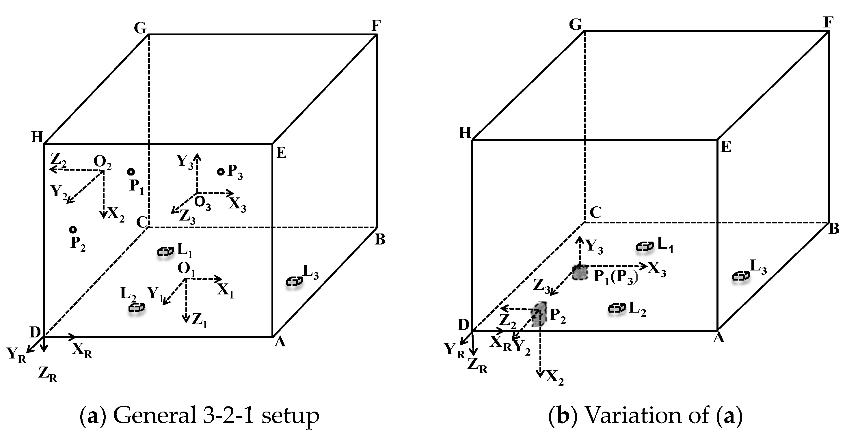
Figure 2a,b show the orthogonal 3-2-1 fixturing setup by a plane and three locators [15,20]. Figure 2a shows a general 3-2-1 layout. Surface ABCD is defined as the primary datum plane; this surface constrains two rotational and one translational motion. Surface CDHG is defined as the secondary datum plane; this surface constrains one rotational and one translational motion. Surface BCGF is defined as the tertiary datum plane; it constrains the last translational motion. The current SoV model based on DMVs can predict variation propagation for MMPs with this kind of orthogonal 3-2-1 fixturing setup via a plane and three locators.
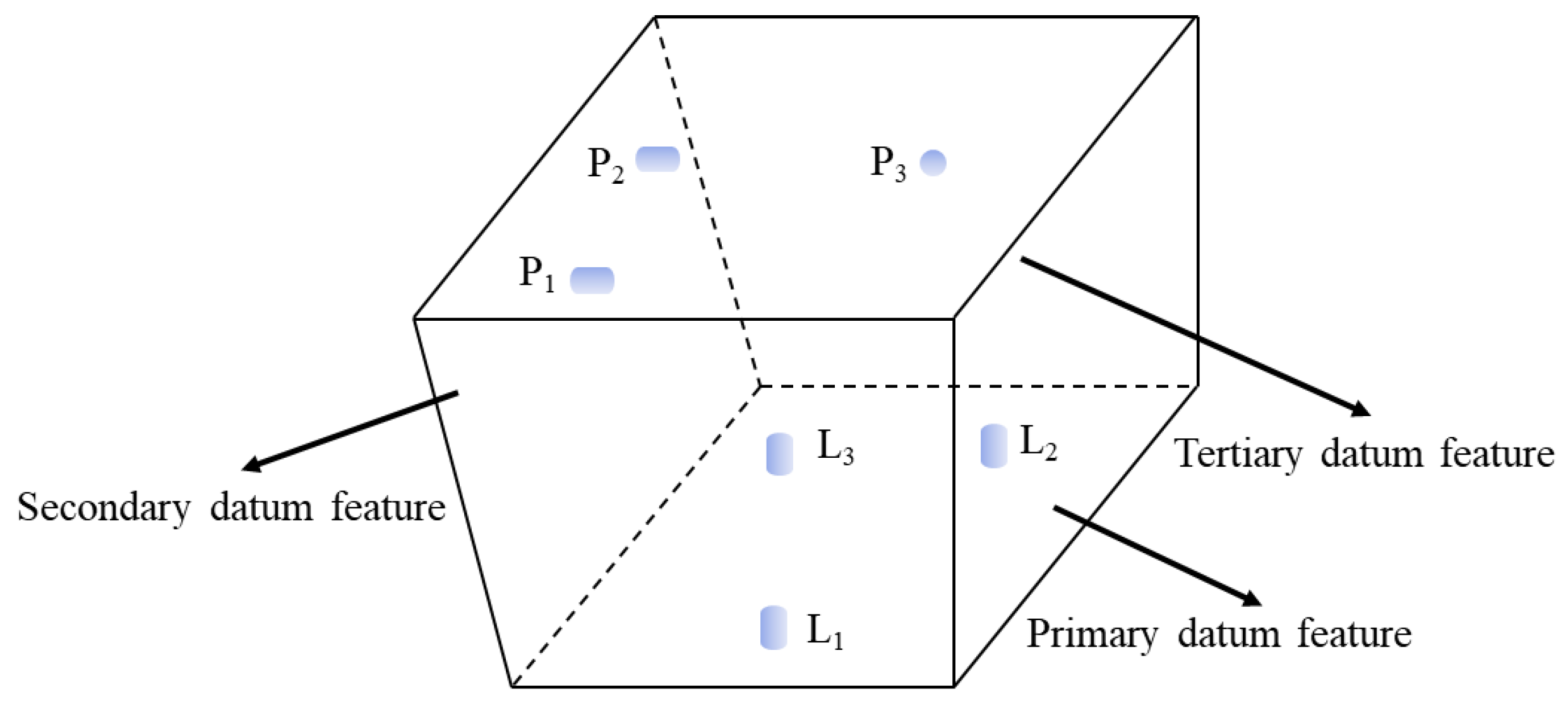
However, the current SoV model based on DMVs cannot handle problems for some complicated workpieces machined in MMPs with non-orthogonal 3-2-1 fixture layouts. As shown in Figure 3, the primary datum plane, the secondary datum plane, and the tertiary datum plane are not orthogonal to each other.

2.2. Datum Error Model

Note that points L 1 , L 2 , and L 3 be the datum points on the primary datum plane. P 1 and P 2 are the datum points on the secondary datum plane. P 3 is the datum point on the tertiary datum plane. The coordinates of these datum locating points in the actual fixture coordinate system (FCS) are P 1 1 , P 2 1 , P 3 1 , P 4 1 , P 5 1 , and P 6 1 , respectively.
Note that p ˜ i 1 = p i 1 T 1 T = p i x 1 p i y 1 p i z 1 1 T , (i = 1, 2, 3, 4, 5, 6). The coordinate of p ˜ i 1 with respect to the FCS can be transformed to the coordinate of p ˜ i d 1 with respect to locating the primary datum feature coordinate system (DFS) by using the homogeneous transformation matrix. The HTM between these two coordinate systems is shown in Appendix A [28]. The transformation process of coordinates of these six locating points is rep-resented as:
H 0 d 1 H 1 0 p ˜ 1 1 = p ˜ 1 d 1   H 0 d 1 H 1 0 p ˜ 2 1 = p ˜ 2 d 1   H 0 d 1 H 1 0 p ˜ 3 1 = p ˜ 3 d 1 H 0 d 2 H 1 0 p ˜ 4 1 = p ˜ 4 d 2   H 0 d 2 H 1 0 p ˜ 5 1 = p ˜ 5 d 2   H 0 d 3 H 1 0 p ˜ 6 1 = p ˜ 6 d 3
Each locator touches its corresponding datum feature, and according to the deterministic locating, when the point of a fixture locator touches the corresponding point of a datum feature, the Z coordinate value of each locator in the datum coordinate system should be zero [15]. Take the first line of Equation (1) as an example; the third element of p ˜ 1 d 1 should be zero in order to guarantee touching; then, we have H 0 d 1 H 1 0 p ˜ 1 1   ( 3 ) = 0 .   ( i ) represents the ith element of the column vectors. The homogeneous transformation matrix between the FCS and the reference coordinate system (RCS) is denoted as H 1 0 ; then, we have
H 1 0 = H 1 0 ( Δ 1 1 + I )
where H 1 0 is the homogeneous transformation matrix between the nominal fixture coordinate system 0FCS and RCS; Δ 1 1 = θ ^ 1 1 d 1 1 0 I is the homogeneous transformation matrix between the FCS and 0FCS; I is the corresponding identity matrix.
Similarly, the homogeneous transformation matrix between the actual locating datum feature coordinate system C S d 1 and RCS can be denoted as
H d 1 0 = H d 1 0 H d 1 d 1
where H d 1 0 is the homogeneous transformation matrix between the nominal locating datum feature coordinate system and RCS. H d 1 d 1 is the actual locating datum feature coordinate system C S d 1 and the nominal locating datum feature coordinate system C S d 1 . By calculating the inverse matrix of H d 1 0 , Equation (3) can be obtained as
H 0 d 1 = ( H d 1 0 ) 1 = ( H d 1 0 H d 1 d 1 ) 1 = ( H d 1 d 1 ) 1 H 0 d 1 = ( Δ d 1 d 1 + I ) H 0 d 1
Substituting Equations (2) and (3) into equation H 0 d 1 H 1 0 p ˜ 1 1 , Equation (4) can be obtained as
H 0 d 1 H 1 0 p ˜ 1 1 = ( Δ d 1 d 1 + I ) H 0 d 1 H 1 0 ( Δ 1 1 + I ) p ˜ 1 1
H 0 d 1 H 1 0 p ˜ 1 1   ( 3 ) = 0 can change to ( Δ d 1 d 1 + I ) H 0 d 1 H 1 0 ( Δ 1 1 + I ) p ˜ 1 1 ( 3 ) = 0 based on Equation (4). Equation (4) can be rewritten as
H 0 d 1 H 1 0 p ˜ 1 1 ( 3 ) ( Δ d 1 d 1 H 1 d 1 + H 1 d 1 Δ 1 1 ) p ˜ 1 1 ( 3 )
where Δ d 1 d 1 , H 1 d 1 , Δ 1 1 , and p ˜ 1 1 can be expressed as follows:
Δ d 1 d 1 = θ ^ d 1 d 1 d d 1 d 1 0 1 = 0 θ d 1 z d 1 θ d 1 y d 1 d d 1 x d 1 θ d 1 z d 1 0 θ d 1 x d 1 d d 1 y d 1 θ d 1 y d 1 θ d 1 x d 1 0 d d 1 z d 1 0 0 0 1
H 1 d 1 = n 1 d 1 o 1 d 1 a 1 d 1 t 1 d 1 0 0 0 1 = n 1 x d 1 o 1 x d 1 a 1 x d 1 t 1 x d 1 n 1 y d 1 o 1 y d 1 a 1 y d 1 t 1 y d 1 n 1 z d 1 o 1 z d 1 a 1 z d 1 t 1 z d 1 0 0 0 1
Δ 1 1 = θ ^ 1 1 d 1 1 0 1 = 0 θ 1 z 1 θ 1 y 1 d 1 x 1 θ 1 z 1 0 θ 1 x 1 d 1 y 1 θ 1 y 1 θ 1 x 1 0 d 1 z 1 0 0 0 1
p ˜ 1 1 = p 1 1 1 T
By solving ( Δ d 1 d 1 H 1 d 1 + H 1 d 1 Δ 1 1 ) p ˜ 1 1 ( 3 ) , Equation (10) can be written as
Δ d 1 d 1 H 1 d 1 p ˜ 1 1 ( 3 ) = H 1 d 1 Δ 1 1 p ˜ 1 1 ( 3 )
Substituting Equations (6)–(9) into Equation (10), Equations (11) and (12) can be obtained as follows:
Δ d 1 d 1 H 1 d 1 p ˜ 1 1 ( 3 ) = [ θ d 1 d 1 × n 1 d 1 ] ( 3 ) [ θ d 1 d 1 × o 1 d 1 ] ( 3 ) [ θ d 1 d 1 × a 1 d 1 ] ( 3 ) [ θ d 1 d 1 × t 1 d 1 + d d 1 d 1 ] ( 3 ) p ˜ 1 1
H 1 d 1 Δ 1 1 p ˜ 1 1 ( 3 ) = [ a d 1 1 ] T   [ p 1 1 × a d 1 1 ] T x 1 1
where x 1 1 is the corresponding differential motion vector of differential motion matrix Δ 1 1 .
Substituting Equations (11) and (12) into Equation (10) yields
  [ a d 1 1 ] T   [ p 1 1 × a d 1 1 ] T x 1 1 = [ θ d 1 d 1 × n 1 d 1 ] ( 3 ) [ θ d 1 d 1 × o 1 d 1 ] ( 3 ) [ θ d 1 d 1 × a 1 d 1 ] ( 3 ) [ θ d 1 d 1 × t 1 d 1 + d d 1 d 1 ] ( 3 ) p ˜ 1 1
Similarly, by solving the other five points, P 2 , P 3 , P 4 , P 5 , and P 6 in Equation (10), we have
[   [ a d 1 1 ] T   [ p 1 1 × a d 1 1 ] T   [ a d 1 1 ] T   [ p 2 1 × a d 1 1 ] T   [ a d 1 1 ] T   [ p 3 1 × a d 1 1 ] T   [ a d 2 1 ] T   [ p 4 1 × a d 2 1 ] T   [ a d 2 1 ] T   [ p 5 1 × a d 2 1 ] T   [ a d 3 1 ] T   [ p 6 1 × a d 3 1 ] T ] x 1 1 = [ [ [ θ d 1 d 1 × n 1 d 1 ] ( 3 ) [ θ d 1 d 1 × o 1 d 1 ] ( 3 ) [ θ d 1 d 1 × a 1 d 1 ] ( 3 ) [ θ d 1 d 1 × t 1 d 1 + d d 1 d 1 ] ( 3 ) ] p ˜ 1 1 [ [ θ d 1 d 1 × n 1 d 1 ] ( 3 ) [ θ d 1 d 1 × o 1 d 1 ] ( 3 ) [ θ d 1 d 1 × a 1 d 1 ] ( 3 ) [ θ d 1 d 1 × t 1 d 1 + d d 1 d 1 ] ( 3 ) ] p ˜ 2 1 [ [ θ d 1 d 1 × n 1 d 1 ] ( 3 ) [ θ d 1 d 1 × o 1 d 1 ] ( 3 ) [ θ d 1 d 1 × a 1 d 1 ] ( 3 ) [ θ d 1 d 1 × t 1 d 1 + d d 1 d 1 ] ( 3 ) ] p ˜ 3 1 [ [ θ d 2 d 2 × n 1 d 2 ] ( 3 ) [ θ d 2 d 2 × o 1 d 2 ] ( 3 ) [ θ d 2 d 2 × a 1 d 2 ] ( 3 ) [ θ d 2 d 2 × t 1 d 2 + d d 2 d 2 ] ( 3 ) ] p ˜ 4 1 [ [ θ d 2 d 2 × n 1 d 2 ] ( 3 ) [ θ d 2 d 2 × o 1 d 2 ] ( 3 ) [ θ d 2 d 2 × a 1 d 2 ] ( 3 ) [ θ d 2 d 2 × t 1 d 2 + d d 2 d 2 ] ( 3 ) ] p ˜ 5 1 [ [ θ d 3 d 3 × n 1 d 3 ] ( 3 ) [ θ d 3 d 3 × o 1 d 3 ] ( 3 ) [ θ d 3 d 3 × a 1 d 3 ] ( 3 ) [ θ d 3 d 3 × t 1 d 3 + d d 3 d 3 ] ( 3 ) ] p ˜ 6 1 ]
By knowing a = a 1 a 2 a 3 T and b = b 1 b 2 b 3 T , Equation (15) will be yielded as
a × b = ( a 2 b 3 a 3 b 2 ) i + ( a 3 b 1 a 1 b 3 ) j + ( a 1 b 2 a 2 b 1 ) k
The third element of a × b ( 3 ) is shown as Equation (16).
a × b ( 3 ) = a 1 b 2 a 2 b 1
As to p 1 1 , according to Equations (15) and (16), the expression of   [ a d 1 1 ] T   [ p 1 1 × a d 1 1 ] T and [ θ d 1 d 1 × n 1 d 1 ] ( 3 ) [ θ d 1 d 1 × o 1 d 1 ] ( 3 ) [ θ d 1 d 1 × a 1 d 1 ] ( 3 ) [ θ d 1 d 1 × t 1 d 1 + d d 1 d 1 ] ( 3 ) p ˜ 1 1 can be rewritten as Equations (17) and (18) as follows:
[ a d 1 1 ] T   [ p 1 1 × a d 1 1 ] T = a d 1 x 1 a d 1 y 1 a d 1 z 1 L 1 y a d 1 z 1 L 1 z a d 1 y 1 L 1 z a d 1 x 1 L 1 x a d 1 z 1 L 1 x a d 1 y 1 L 1 y a d 1 x 1
[ [ θ d 1 d 1 × n 1 d 1 ] [ θ d 1 d 1 × o 1 d 1 ] [ θ d 1 d 1 × a 1 d 1 ] [ θ d 1 d 1 × t 1 d 1 + d d 1 d 1 ] ] p ˜ 1 1 = [ θ d 1 x d 1 n 1 y d 1 θ d 1 y d 1 n 1 x d 1 θ d 1 x d 1 o 1 y d 1 θ d 1 y d 1 o 1 x d 1 θ d 1 x d 1 a 1 y d 1 θ d 1 y d 1 a 1 x d 1 θ d 1 x d 1 t 1 y d 1 θ d 1 y d 1 t 1 x d 1 + d d 1 z d 1 ] p ˜ 1 1
By solving the other five points in Equation (14), similarly, Equation (14) can be rewritten as the following Equation (19):
[ a d 1 x 1 a d 1 y 1 a d 1 z 1 L 1 y a d 1 z 1 L 1 z a d 1 y 1 L 1 z a d 1 x 1 L 1 x a d 1 z 1 L 1 x a d 1 y 1 L 1 y a d 1 x 1 a d 1 x 1 a d 1 y 1 a d 1 z 1 L 2 y a d 1 z 1 L 2 z a d 1 y 1 L 2 z a d 1 x 1 L 2 x a d 1 z 1 L 2 x a d 1 y 1 L 2 y a d 1 x 1 a d 1 x 1 a d 1 y 1 a d 1 z 1 L 3 y a d 1 z 1 L 3 z a d 1 y 1 L 3 z a d 1 x 1 L 3 x a d 1 z 1 L 3 x a d 1 y 1 L 3 y a d 1 x 1 a d 2 x 1 a d 2 y 1 a d 2 z 1 p 1 y a d 2 z 1 p 1 z a d 2 y 1 p 1 z a d 2 x 1 p 1 x a d 2 z 1 p 1 x a d 2 y 1 p 1 y a d 2 x 1 a d 2 x 1 a d 2 y 1 a d 2 z 1 p 2 y a d 2 z 1 p 2 z a d 2 y 1 p 2 z a d 2 x 1 p 2 x a d 2 z 1 p 2 x a d 2 y 1 p 2 y a d 2 x 1 a d 3 x 1 a d 3 y 1 a d 3 z 1 p 3 y a d 3 z F p 3 z a d 3 y 1 p 3 z a d 3 x 1 p 3 x a d 3 z 1 p 3 x a d 3 y 1 p 3 y a d 3 x 1 ] x 1 1 = [ [ θ d 1 x d 1 n 1 y d 1 θ d 1 y d 1 n 1 x d 1 θ d 1 x d 1 o 1 y d 1 θ d 1 y d 1 o 1 x d 1 θ d 1 x d 1 a 1 y d 1 θ d 1 y d 1 a 1 x d 1 θ d 1 x d 1 t 1 y d 1 θ d 1 y d 1 t 1 x d 1 + d d 1 z d 1 ] p ˜ 1 1 [ θ d 1 x d 1 n 1 y d 1 θ d 1 y d 1 n 1 x d 1 θ d 1 x d 1 o 1 y d 1 θ d 1 y d 1 o 1 x d 1 θ d 1 x d 1 a 1 y d 1 θ d 1 y d 1 a 1 x d 1 θ d 1 x d 1 t 1 y d 1 θ d 1 y d 1 t 1 x d 1 + d d 1 z d 1 ] p ˜ 2 1 [ θ d 1 x d 1 n 1 y d 1 θ d 1 y d 1 n 1 x d 1 θ d 1 x d 1 o 1 y d 1 θ d 1 y d 1 o 1 x d 1 θ d 1 x d 1 a 1 y d 1 θ d 1 y d 1 a 1 x d 1 θ d 1 x d 1 t 1 y d 1 θ d 1 y d 1 t 1 x d 1 + d d 1 z d 1 ] p ˜ 3 1 [ θ d 2 x d 2 n 1 y d 2 θ d 2 y d 2 n 1 x d 2 θ d 2 x d 2 o 1 y d 2 θ d 2 y d 2 o 1 x d 2 θ d 2 x d 2 a 1 y d 2 θ d 2 y d 2 a 1 x d 2 θ d 2 x d 2 t 1 y d 2 θ d 2 y d 2 t 1 x d 2 + d d 2 z d 2 ] p ˜ 4 1 [ θ d 2 x d 2 n 1 y d 2 θ d 2 y d 2 n 1 x d 2 θ d 2 x d 2 o 1 y d 2 θ d 2 y d 2 o 1 x d 2 θ d 2 x d 2 a 1 y d 2 θ d 2 y d 2 a 1 x d 2 θ d 2 x d 2 t 1 y d 2 θ d 2 y d 2 t 1 x d 2 + d d 2 z d 2 ] p ˜ 5 1 [ θ d 3 x d 3 n 1 y d 3 θ d 3 y d 3 n 1 x d 3 θ d 3 x d 3 o 1 y d 3 θ d 3 y d 3 o 1 x d 3 θ d 3 x d 3 a 1 y d 3 θ d 3 y d 3 a 1 x d 3 θ d 3 x d 3 t 1 y d 3 θ d 3 y d 3 t 1 x d 3 + d d 3 z d 3 ] p ˜ 6 1 ] .
Equation (19) includes two parts: the locating parameters and the locating datum errors ( x d 1 d 1 , x d 2 d 2 and x d 3 d 3 ). For sake of simplicity, the locating parameters and locating datum errors are separated as Equation (20).
T x 1 1 = T 1 x d 1 d 1 + T 2 x d 2 d 2 + T 3 x d 3 d 3
where
T = [ a d 1 x 1 a d 1 y 1 a d 1 z 1 L 1 y a d 1 z 1 L 1 z a d 1 y 1 L 1 z a d 1 x 1 L 1 x a d 1 z 1 L 1 x a d 1 y 1 L 1 y a d 1 x 1 a d 1 x 1 a d 1 y 1 a d 1 z 1 L 2 y a d 1 z 1 L 2 z a d 1 y 1 L 2 z a d 1 x 1 L 2 x a d 1 z 1 L 2 x a d 1 y 1 L 2 y a d 1 x 1 a d 1 x 1 a d 1 y 1 a d 1 z 1 L 3 y a d 1 z 1 L 3 z a d 1 y 1 L 3 z a d 1 x 1 L 3 x a d 1 z 1 L 3 x a d 1 y 1 L 3 y a d 1 x 1 a d 2 x 1 a d 2 y 1 a d 2 z 1 p 1 y a d 2 z 1 p 1 z a d 2 y 1 p 1 z a d 2 x 1 p 1 x a d 2 z 1 p 1 x a d 2 y 1 p 1 y a d 2 x 1 a d 2 x 1 a d 2 y 1 a d 2 z 1 p 2 y a d 2 z 1 p 2 z a d 2 y 1 p 2 z a d 2 x 1 p 2 x a d 2 z 1 p 2 x a d 2 y 1 p 2 y a d 2 x 1 a d 3 x 1 a d 3 y 1 a d 3 z 1 p 3 y a d 3 z F p 3 z a d 3 y 1 p 3 z a d 3 x 1 p 3 x a d 3 z 1 p 3 x a d 3 y 1 p 3 y a d 3 x 1 ]
T 1 = [ 0 0 1 n 1 y d 1 L 1 x + o 1 y d 1 L 1 y + a 1 y d 1 L 1 z + t 1 y d 1 ( n 1 x d 1 L 1 x + o 1 x d 1 L 1 y + a 1 x d 1 L 1 z + t 1 x d 1 ) 0 0 0 1 n 1 y d 1 L 2 x + o 1 y d 1 L 2 y + a 1 y d 1 L 2 z + t 1 y d 1 ( n 1 x d 1 L 2 x + o 1 x d 1 L 2 y + a 1 x d 1 L 2 z + t 1 x d 1 ) 0 0 0 1 n 1 y d 1 L 3 x + o 1 y d 1 L 3 y + a 1 y d 1 L 3 z + t 1 y d 1 ( n 1 x d 1 L 3 x + o 1 x d 1 L 3 y + a 1 x d 1 L 3 z + t 1 x d 1 ) 0 0 0 0 0 0 0 0 0 0 0 0 0 0 0 0 0 0 0 ]
T 2 = [ 0 0 0 0 0 0 0 0 0 0 0 0 0 0 0 0 0 0 0 0 1 n 1 y d 2 p 1 x + o 1 y d 2 p 1 y + a 1 y d 2 p 1 z + t 1 y d 2 ( n 1 x d 2 p 1 x + o 1 x d 2 p 1 y + a 1 x d 2 p 1 z + t 1 x d 2 ) 0 0 0 1 n 1 y d 2 p 2 x + o 1 y d 2 p 2 y + a 1 y d 2 p 2 z + t 1 y d 2 ( n 1 x d 2 p 2 x + o 1 x d 2 p 2 y + a 1 x d 2 p 2 z + t 1 x d 2 ) 0 0 0 0 0 0 0 ]
T 3 = 0 0 0 0 0 0 0 0 0 0 0 0 0 0 0 0 0 0 0 0 0 0 0 0 0 0 0 0 0 0 0 0 1 n 1 y d 3 p 3 x + o 1 y d 3 p 3 y + a 1 y d 3 p 3 z + t 1 y d 3 ( n 1 x d 3 p 3 x + o 1 x d 3 p 3 y + a 1 x d 3 p 3 z + t 1 x d 3 ) 0
By multiplying the inverse matrix T - 1 of T on both sides of Equation (20), then Equation (25) can be obtained as:
x 1 1 = T - 1 T 1 x d 1 d 1 + T - 1 T 2 x d 2 d 2 + T - 1 T 3 x d 3 d 3
Denoting A 2 ( k ) = T 1 T 2 T 3 , T 1 = T - 1 T 1 , T 2 = T - 1 T 2 , and T 3 = T - 1 T 3 , Equation (25) will change to Equation (26):
x 1 1 = A 2 ( k ) x d 1 d 1 x d 2 d 2 x d 3 d 3 T
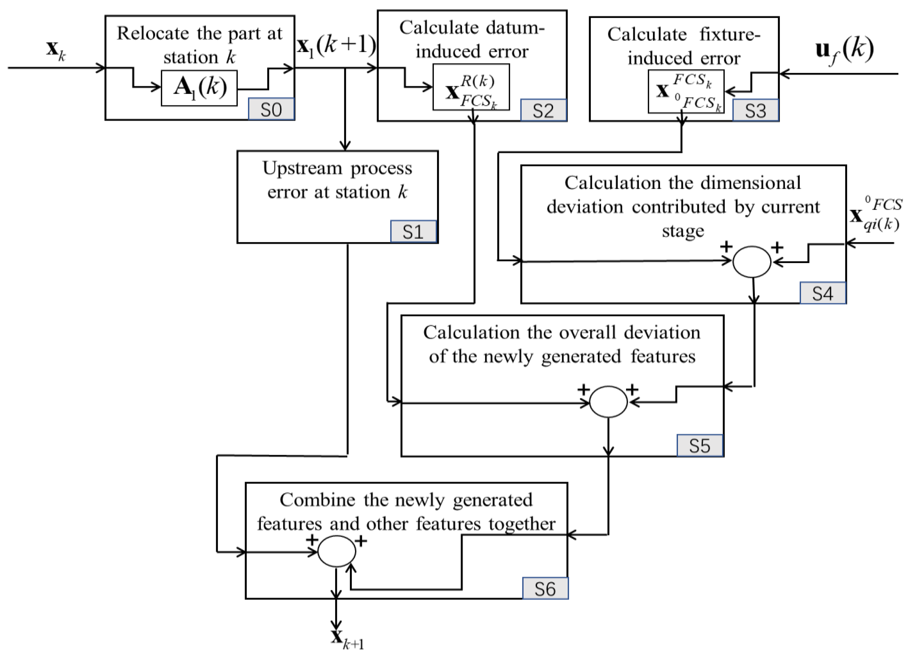
The steps of the derivation of the variation propagation model for MMPs is shown in Figure 4.

2.3. Time-Dependent Variations

The wear of the fixture locator is another important factor affecting a part’s dimensional quality. The wear of the fixture locator will result in a loss of the axial depth of the cut that generates dimensional errors. The wear of the fixture locator is a time-varying variation; the amount of wear increases with processing time. Due to different locators of fixtures with different contacting positions and cutting forces, different locators have different wear rates. The fixture locator wear is represented as
u f ( k )   = f ( Δ u f 1 ) ( k )   f ( Δ u f 2 ) ( k )   f ( Δ u f 3 ) ( k )   f ( Δ u f 4 ) ( k )   f ( Δ u f 5 ) ( k )   f ( Δ u f 6 ) ( k )   T
where f ( Δ u f i ) ( k )   is a function that describes the locator wear due to the clamping force and cutting force. The wear function of each locator can be obtained through experimentation.
At stage k, another machining-induced variation is the cutting tool path error, which includes cutting-force-induced variation x C k S k , geometric-thermal variation in machine–tool axes x A k n F k 0 , spindle thermal variation x S k A k n , and cutting-tool-wear-induced variations x q i C k . The total cutting-tool path error u m ( k ) defined will be affected by x A k n F k 0 , x S k A k n , x C k S k , and x q i C k in the chain. u m ( k ) as a function of all CSs’ deviations can be expressed as
u m ( k ) = T q i ( k ) C k ( T C k S k ( T S k A k n x A k n F k 0 + x S k A k n ) + x C k S k ) + x q i ( k ) C k
where T q i ( k ) C k , T C k S k , and T S k A k n are the matrices to describe the transition of differential motion vectors and can be found in [17].
Solving the above equations, the state space model for MMPs can be obtained as follows:
x 1 1 ( k ) = [ A 1 ( k ) + A 5 ( k ) A 4 ( k ) A 2 ( k ) A 1 ( k ) ] x 1 1 ( k 1 ) + [ A 1 ( k ) A 4 ( k ) A 3 ( k )                     A 5 ( k ) ] u f ( k ) u m ( k ) + w ( k )
where A 1 ( k ) is the relocating matrix, A 2 ( k ) is the datum-induced error matrix, A 3 ( k ) is the fixture-induced error matrix, A 4 ( k ) is an auxiliary matrix to calculate the machining error and the dimensional deviation contributed by the current stage, and A 5 ( k ) is the selector matrix. The expressions of matrices A 1 ( k ) , A 3 ( k ) , A 4 ( k ) , and A 5 ( k ) are listed in the references of [15,17].
The equivalent fixture error concept based on DMVs is applied to calculate the total compensation amount. By this, locators will be adjusted under their corresponding amount.
c ( k + 1 ) = A 4 ( k ) A 3 ( k )   [ Δ d ( k ) + Δ f ( k ) + Δ m ( k ) + Δ w ( k ) ]
where Δ d ( k ) , Δ f ( k ) , Δ m ( k ) , and Δ w ( k ) are the equivalent fixture errors of datum error, fixture error, machine tool path error, and the other errors, correspondingly. For details, readers can refer to references [21,33].

2.4. Percentage Contributions for the Modified Model

The error percentage contribution reflects the contribution of each error source to the total machining errors. The real value of each error source will be used to calculate the error percentage contribution. The machining error caused by each error source can be calculated using Equation (29). The datum error, fixture error, and machine tool path error are calculated as follows:
x d = [ A 1 ( k ) + A 5 ( k ) A 4 ( k ) A 2 ( k ) A 1 ( k ) ] x 1 1 ( k 1 )
x f = A 1 ( k ) A 4 ( k ) A 3 ( k ) u f ( k )
x m = u m ( k )
where x d , x f , and x m are the machining errors caused by a datum error, fixture error, and machine tool path error, respectively.
The actual values may deviate from the nominal values; the errors of Equations (27)–(33) are represented by the deviation of their actual places with respect to their nominal places. The corresponding error percentage contribution of the datum error, fixture error, and machine tool path error are modeled as Equations (34)–(36).
P C d = [ A 1 ( k ) + A 5 ( k ) A 4 ( k ) A 2 ( k ) A 1 ( k ) ] x 1 1 ( k 1 ) / x 1 1 ( k )
P C f = A 1 ( k ) A 4 ( k ) A 3 ( k ) u f ( k ) / x 1 1 ( k )
P C m = u m ( k ) / x 1 1 ( k )
where P C d , P C f , and P C m are the error percentage contributions of datum error, fixture error, and machine tool path error, respectively.
The machining tool path error u m ( k ) can be further decomposed as the following equations:
u m 1 ( k ) = x q i ( k ) C k
u m 2 ( k ) = T q i ( k ) C k x C k S k
u m 3 ( k ) = T q i ( k ) C k T C k S k x S k a k n
u m 4 ( k ) = T q i ( k ) C k T C k S k T S k A k n x A k n F k 0
where u m 1 ( k ) , u m 2 ( k ) , u m 3 ( k ) , and u m 4 ( k ) are machining errors caused by cutting-tool-wear-induced variation, cutting-force-induced variation, spindle thermal variation, and the geometric-thermal variation in machine–tool axes, respectively.
The corresponding error percentage contribution of the datum error, fixture error, and the machining tool path error are modeled as Equations (41)–(44).
P C m 1 = u m 1 ( k ) / x ( k )
P C m 2 = u m 2 ( k ) / x ( k )
P C m 3 = u m 3 ( k ) / x ( k )
P C m 4 = u m 4 ( k ) / x ( k )
where P C m 1 , P C m 2 , P C m 3 , and P C m 4 are the error percentage contributions of cutting-tool-wear-induced variation, cutting-force-induced variation, spindle thermal variation, and the geometric-thermal variation in machine–tool axes, respectively.

3. Case Study

3.1. Simulation Case Study

Compared to the SoV model developed by Loose through the kinematic analysis method for MMPs with general non-orthogonal fixture layouts, the modified SoV model can solve the machining-induced variations, such as spindle thermal variation, cutting-force-induced variation, cutting-tool-wear-induced variations, and the geometric-thermal variation in machine–tool axes. Although the current SoV model based on DMVs can deal with machining-induced variations, it cannot be applied to a general non-orthogonal fixture layout.
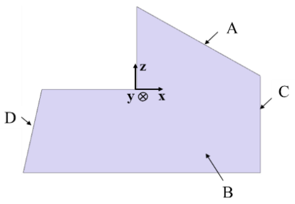
The simulation case study will adopt a machining process with the non-orthogonal 3-2-1 layouts shown in Figure 5. For the sake of simplicity, only one feature will be machined on the workpiece through end milling. The machining step is to mill feature D. The locating datums are feature A, feature B, and feature C. This fixture layout is not a traditional orthogonal 3-2-1 layout.
Datum features, the locator coordinate in the FCS, and the outgoing normal direction of feature in the FCS are listed in Table 1. For the sake of simplicity, the FCS is taken to represent the part coordinate system (PCS). The nominal locations and orientations of the locators, expressed in the FCS, are shown in Table 2.
For this machining process case, these errors are listed in Table 3.
The machining error of feature D will be predicted. The machining error caused by the datum error, fixture error, and machine tool path error is predicted as
x = 0.0350 0.0210 0.0448 0.0001 0 0.0003 T
In order to illustrate the time-varying variations, the feature deviation due to the spindle thermal expansion will be introduced. For spindle thermal variations, only the spindle thermal expansion in the z direction was considered during the spindle warm-up. For the simulation, this paper will introduce the mathematical relationship model between feature deviation and the spindle temperature from reference [17] as follows:
y = 0.0052 x + 0.0816
where x is the spindle temperature, and y refers to the feature deviation. All of the machining conditions are assumed to be the same as reference [17].
By using the above fixture errors and datum errors, the deviations due to spindle temperature will be introduced. The temperatures are set as 15 °C and 30 °C. Substituting these temperatures into Equation (31), the deviations caused by spindle thermal variations are calculated as 0.0036 mm and −0.0744 mm for 15 °C and 30 °C, respectively. Substituting the errors from Table 3 and the deviations of 0.0036 mm and −0.0744 mm caused by spindle temperature into Equations (28) and (29), the total deviations in the z direction are −0.0412 mm and −0.1192 mm, respectively.
As can be seen, different temperatures have different impacts on the machining error. When the temperature is 15 °C, the machining error in the z direction will additionally increase by 0.0036 mm. The total machining error in the z direction will change from −0.0448 mm to −0.0412 mm. When the temperature changes to 30 °C, the machining error in the z direction will additionally increase by −0.0744 mm. Then, the total machining error in the z direction will change from −0.0448 mm to −0.1192 mm. The absolute value of the additional machining error caused by 30 °C is higher than that caused by 15 °C.

3.2. Experimental Case Study

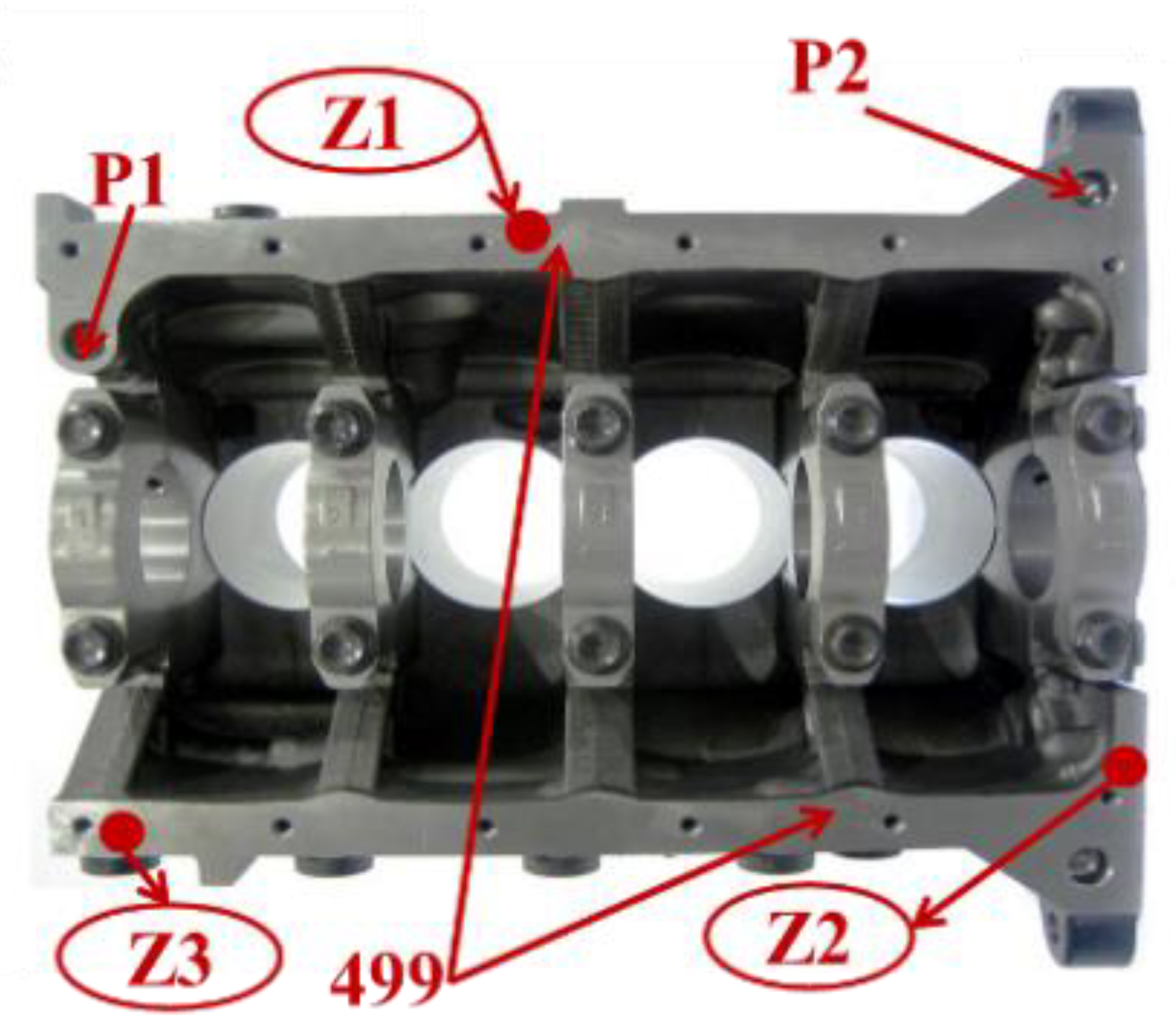
A B12 engine block is used to be machined to validate the proposed model. The key features of this block are shown in Figure 6. Feature 499 is the primary locating datum. Feature 399 is the machined face. This operation is to mill feature 399. Z1, Z2, and Z3 are the locating points in the primary datum feature. Hole P1 and P2 are the locating holes in the secondary datum feature and the tertiary datum feature, respectively.
The nominal positions of the locators and orientations of key features in the FCS are listed in Table 4. For the sake of simplicity, the FCS is taken to be the same as the PCS. The location of the machined feature is [−60, −3, −186].
For this machining process case, the machining error sources and their corresponding errors are measured in a real production line and listed in Table 5. The machine path tool error is set as zero to ensure a nominal machining process.
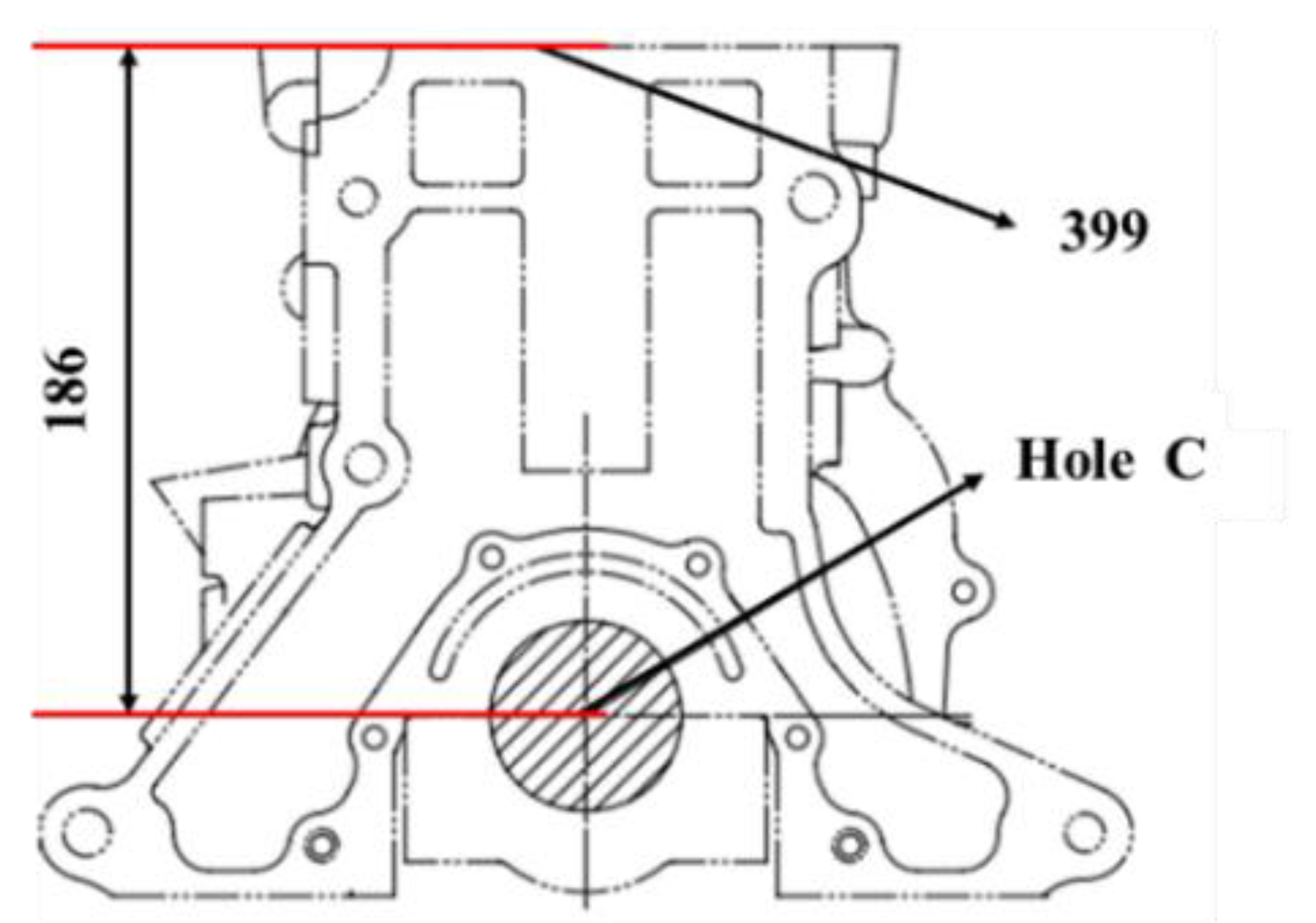
The nominal distance from feature 399 to the axis of hole C is 186 mm, as shown in Figure 7. The distance from feature 399 to the axis of hole C will be measured via CMM after milling process as 186.039 mm. The machining error and distance are predicted as 0.047 mm and 186.047 mm, respectively. The difference between the measured result and the predicted result is 0.008 mm; this is very small. This difference may be caused by the repeated positioning accuracy of the machine tool. The error percent contribution of the fixture error source in the z direction is 69.5%. The error percent contribution of the primary locating datum error source in the z direction is 30.5%. As can be seen, the fixture error is the main error for the machining error.
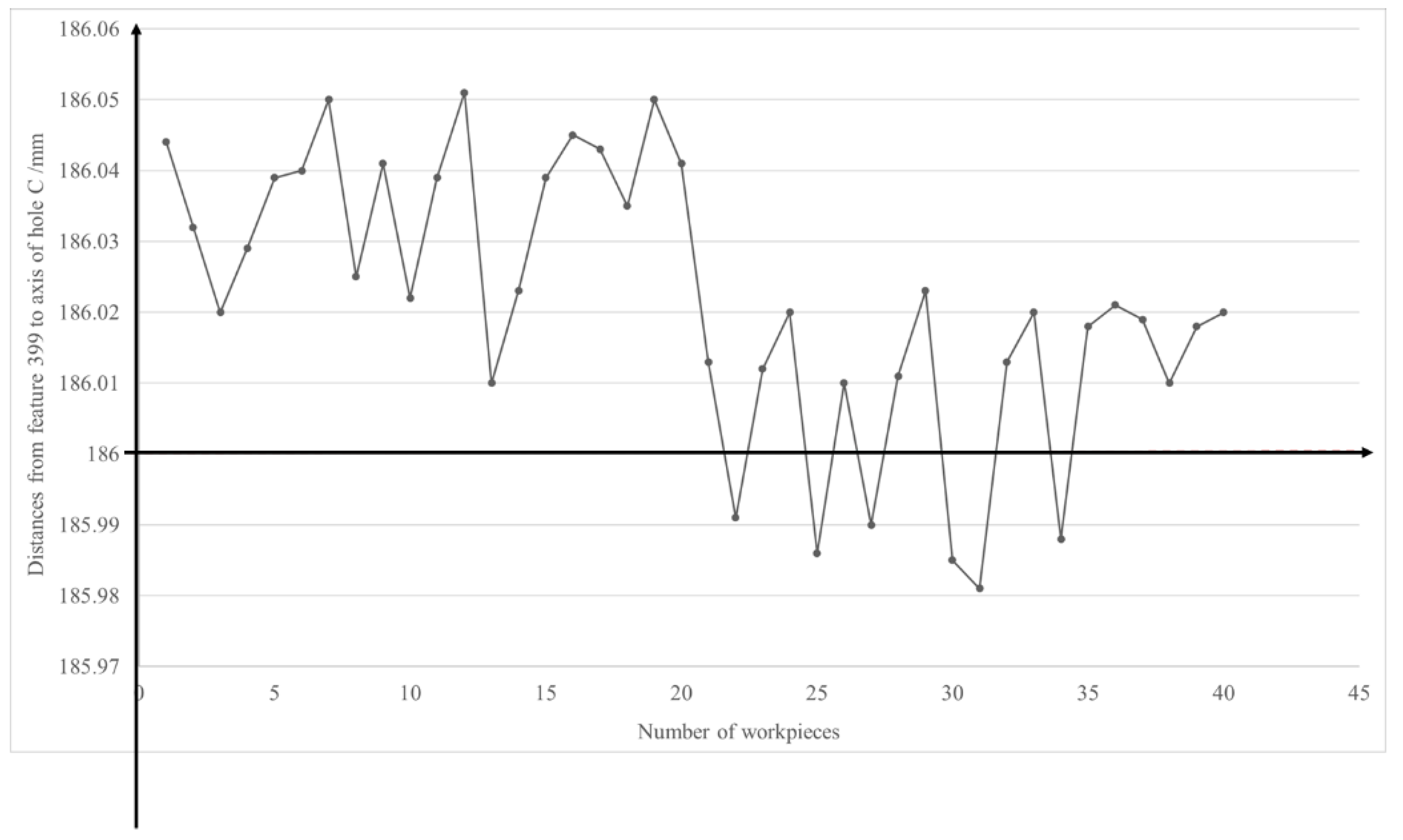
In the same real production line, after 20 blocks are machined, the distances from feature 399 to the axis of hole C of 30 blocks are measured before adjusting the fixture locators. Then, the fixture locators are adjusted, and the fixture error will change from 0.02 0.03 0.01 0 0 0 T to 0 0 0 0 0 0 T . As shown in Figure 8, the first twenty distances are measured before adjusting the fixture locators, and the last twenty distances are measured after adjusting the fixture locators.
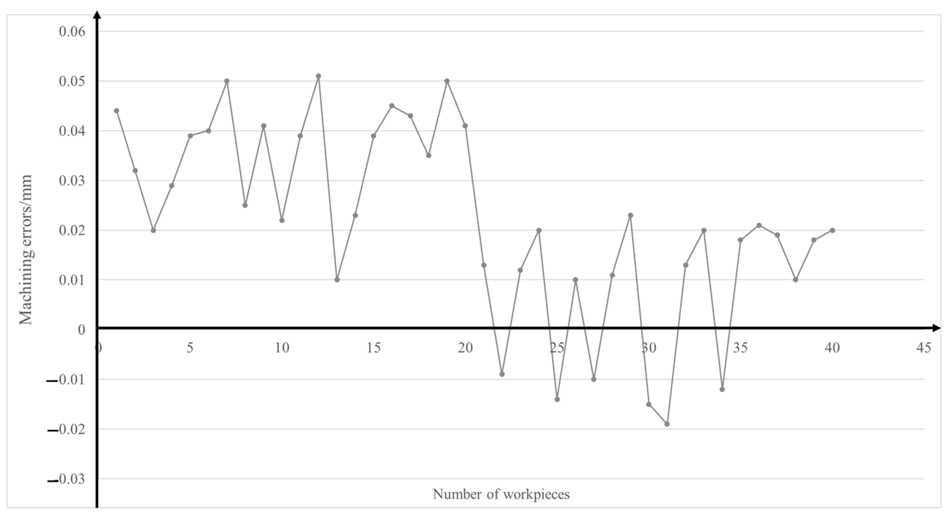
Figure 9 shows the machining errors of these forty blocks. The average machining error in the z direction of the first twenty blocks is 0.0359 mm. Additionally, the average percent contribution of fixture error is calculated as 91.3%. Then, the fixture locators are adjusted to make the fixture error zero. After adjusting the fixture locators, another 20 distances are measured. The average machining error in the z direction of the last twenty blocks is 0.007 mm. As can be seen, after adjusting the fixture locators, the average machining error is reduced 80.5%. In addition, compared with the first twenty blocks, the machining errors of the last twenty blocks are obviously reduced after adjusting the fixture locator.

4. Conclusions

In spite of the success of current SoV methods based on DMVs for variation prediction, current models are limited to orthogonal 3-2-1 fixture layouts. This paper proposes a modified SoV model based on DMVs that can predict machining errors for complex-shaped workpieces in multi-stage machining processes with non-orthogonal 3-2-1 fixture layouts. As a result, the proposed model can notably extend the application field. Error percent contributions are proposed to calculate each error source’s contribution to the total machining error. The error percent contribution reflects the contribution of each error source to the total machining errors. Different error sources have different impacts on the total machining error. Through error percent contributions, the main error sources can be identified. The proposed error prediction methodology for machining process will provide an important method for changing the main machining parameters to produce better-quality parts.
The modified SoV model can extend the application in the following fields, such as machining error prediction for MMPs with non-orthogonal 3-2-1 fixture layouts, machining error compensation, root cause identification for the quality improvement purpose, optimizing for the layout of the fixture locators, and so on. Furthermore, the applicability of the proposed SoV model can be considered as follows: (i) Current SoV models have dealt the 3-2-1 fixture layouts; N-2-1 layouts for MMPs should be addressed in future work. Different from the 3-2-1 layout, the N-2-1 layout has more than three positioning points on the primary datum plane to constrain two rotational and one translational motion and limit the deformation of the part. (ii) More error sources of variation should be considered in the SoV model to improve the accurateness of error prediction.

Author Contributions

Conceptualization, F.Y.; Methodology, F.Y. and Y.X.; Software, X.Z.; Validation, F.Y.; Formal analysis, F.Y.; Investigation, P.Z.; Writing—original draft, F.Y.; Writing—review & editing, J.C.; Funding acquisition, F.Y. and Y.X. All authors have read and agreed to the published version of the manuscript.

Funding

This research was funded by Open Project of Shanghai Key Laboratory of Digital Manufacture for Thin-walled Structures: Grant No. 2019-002; the Natural Science Foundation of Shanghai: grant no. 20ZR1422600; Shanghai Doctoral Unit Cultivation Project—Mechanical Engineering Doctoral Program (0231-A1-5300-23-06007); Science and Technology Development Fund of Pudong New Area: PKX2021-W08. The APC was funded by Open Project of Shanghai Key Laboratory of Digital Manufacture for Thin-walled Structures: Grant No. 2019-002.

Data Availability Statement

There is no research data to share.

Conflicts of Interest

The authors declare no conflict of interest.

Abbreviations

The following abbreviations are used in this manuscript:
FCSFixture coordinate system.
LCSiith local coordinate system.
RCSReference coordinate system. The reference coordinate system is for the features of the workpiece.
HTMHomogeneous transformation matrix.
H i R HTM between RCS and LCSi.
R i R Rotational matrix between RCS and LCSi.
T 1 , T 2 , T 3 Transformation matrices for datum-induced error.
d n R   θ n R   Position and orientation deviation of LCSn from nominal positions with regard to RCS.
d n x R , d n y R , d n z R Three elements of d n R .
θ n x R , θ n y R , θ n z R Three elements of θ n R .
Δ i R Differential transformation matrix of δ H i R .
t n R Vector of the origin of LCSn expressed in RCS.
t n x R , t n y R , t n z R Three elements of t n R .
ω n R Euler rotational angles between RCS and LCSn.
ω n x R , ω n y R , ω n z R Three elements of ω n R .
x n R Differential motion vector representing the deviation of LCS in RCS. It is a stack of d n R and   θ n R and is expressed in LCS.

Appendix A

Local coordinate system i ( L C S i ) is expressed with regard to the RCS through a 4 × 4 HTM H i R . The HTM between these two coordinate systems is
H i R = R i R t i R 0 1
where t i R is the location vector of the origin of the LCS expressed with regard to the RCS. The orientation of L C S i is viewed as firstly rotating around the X axis of the RCS by an angle of α i R   , then rotating the new coordinate system around the new Y R axis by β i R , and finally rotating the new coordinate system around the new Z R axis by γ i R . R i R can be formulated as
R i R = R o t ( X R , α i R ) R o t ( Y R , β i R ) R o t ( Z R , γ i R )
where R o t ( X R , α i R ) = 1 0 0 0 0 cos α i R sin α i R   0 0 sin α i R cos α i R 0 0 0 0 1 , R o t ( Y R , β i R ) = cos β i R 0 sin β i R 0 0 1 0 0 sin β i R 0 cos β i R 0 0 0 0 1 and R o t ( Z R , γ i R ) = cos γ i R sin γ i R 0 0 sin γ i R cos γ i R 0 0 0 0 1 0 0 0 0 1 .

References

  1. Ramesh, R.; Mannan, M.A.; Poo, A.N. Error compensation in machine tools-a review part I: Geometric, cutting-force induced and fixture dependent errors. Int. J. Mach. Tools Manuf. 2000, 40, 1235–1256. [Google Scholar] [CrossRef]
  2. Cai, W.; Hu, S.J.; Yuan, J. A variational method of robust fixture configuration design for 3-Dworkpieces. ASME J. Manuf. Sci. Eng. 1997, 119, 593–602. [Google Scholar] [CrossRef]
  3. Dong, Z.; Jiao, L.; Wang, X.; Liang, Z.; Liu, Z.; Yi, J. FEA-based prediction of machined surface errors for dynamic fixture-workpiece system during milling process. Int. J. Adv. Manuf. Technol. 2016, 85, 299–315. [Google Scholar] [CrossRef]
  4. Ramesh, R.; Mannan, M.A.; Poo, A.N. Variation compensation in machine tools—A review part II: Thermal variations. Int. J. Mach. Tools Manuf. 2000, 40, 1235–1256. [Google Scholar] [CrossRef]
  5. Nguyen, H.T.; Wang, H.; Hu, S.J. Characterization of cutting force induced surface shape variation in face milling using high-definition metrology. J. Manuf. Sci. Eng. Trans. ASME 2013, 135, 41014. [Google Scholar] [CrossRef]
  6. Liu, S.; Jin, S.; Zhang, X.; Chen, K.; Tian, A.; Xi, L. A coupled model for the prediction of surface variation in face milling large-scale workpiece with complex geometry. J. Manuf. Sci. Eng. Trans. ASME 2019, 141, 31009–31014. [Google Scholar] [CrossRef]
  7. Wang, K.; Li, G.L.; Du, S.C.; Xi, L.F.; Xia, T.B. State space modelling of variation propagation in multistage machining processes for variable stiffness structure workpieces. Int. J. Prod. Res. 2020, 59, 4033–4052. [Google Scholar] [CrossRef]
  8. Wang, H.; Huang, Q.; Katz, R. Multi-operational machining processes modeling for sequential root cause identification and measurement reduction. J. Manuf. Sci. Eng. Trans. ASME 2005, 127, 512–521. [Google Scholar] [CrossRef]
  9. Hu, S.J.; Koren, Y. Stream-of-variation theory for automotive body assembly. CIRP Ann. 1997, 46, 1–6. [Google Scholar] [CrossRef]
  10. Jin, J.; Shi, J. State space modeling of sheet metal assembly for dimensional control. J. Manuf. Sci. Eng. 1999, 121, 756–762. [Google Scholar] [CrossRef]
  11. Guo, J.; Li, B.; Liu, Z.; Hong, J.; Wu, X. Integration of geometric variation and part deformation into variation propagation of 3-D assemblies. Int. J. Prod. Res. 2016, 54, 5708–5721. [Google Scholar] [CrossRef]
  12. Gianfranco, G.; Galetto, M.; Franceschini, F. Product complexity and design of inspection strategies for assembly manufacturing processes. Int. J. Prod. Res. 2018, 56, 4056–4066. [Google Scholar]
  13. Zhong, W.; Huang, Y.; Hu, S.J. Modeling variation propagation in machining systems with different configurations. ASME Int. Mech. Eng. Congr. Expo. 2002, 671, 97–106. [Google Scholar]
  14. Huang, Q.; Shi, J.; Yuan, J. Part dimensional error and its propagation modeling in multi-operational machining processes. J. Manuf. Sci. Eng. 2003, 125, 255–262. [Google Scholar] [CrossRef]
  15. Zhou, S.; Huang, Q.; Shi, J. State space modeling of dimensional variation propagation in multistage machining process using differential motion vectors. IEEE Trans. Robot. Autom. 2003, 19, 296–309. [Google Scholar] [CrossRef]
  16. Loose, J.P.; Zhou, S.; Ceglarek, D. Kinematic analysis of dimensional variation propagation for multistage machining processes with general fixture layouts. IEEE Trans. Robot. Autom. 2007, 4, 141–152. [Google Scholar] [CrossRef]
  17. Abellan-Nebot, J.V.; Liu, J.; Subirón, F.R.; Shi, J. State space modeling of variation propagation in multistation machining processes considering machining-induced variations. J. Manuf. Sci. Eng. 2012, 134, 021002. [Google Scholar] [CrossRef]
  18. Abellan-Nebot, J.V.; Liu, J. Variation propagation modeling for multi-station machining processes with fixtures based on locating surfaces. Int. J. Prod. Res. 2013, 51, 4667–4681. [Google Scholar] [CrossRef]
  19. Liu, J.; Shi, J.; Hu, S.J. Quality-assured setup planning based on the stream-of-variation model for multi-stage machining processes. IIE Trans. 2009, 41, 323–334. [Google Scholar] [CrossRef]
  20. Zhang, M.; Djurdjanovic, D.; Ni, J. Diagnosibility and sensitivity analysis for multi-station machining processes. Int. J. Mach. Tools Manuf. 2007, 47, 646–657. [Google Scholar] [CrossRef]
  21. Yang, F.; Xing, Y.; Li, X. A comprehensive error compensation strategy for machining process with general fixture layouts. Int. J. Adv. Manuf. Technol. 2020, 107, 2707–2717. [Google Scholar] [CrossRef]
  22. Du, S.; Yao, X.; Huang, D. Engineering model-based Bayesian monitoring of ramp-up phase of multistage manufacturing process. Int. J. Prod. Res. 2015, 53, 4594–4613. [Google Scholar] [CrossRef]
  23. Djurdjanovic, D.; Ni, J. Stream-of-variation (SoV)-based measurement scheme analysis in multistation machining systems. IEEE Trans. Autom. Sci. Eng. 2006, 3, 407–422. [Google Scholar] [CrossRef]
  24. Qin, Y.; Zhao, L.; Yao, Y.; Xu, D. Multistage machining processes variation propagation analysis based on machining processes weighted network performance. Int. J. Adv. Manuf. Technol. 2011, 55, 487–499. [Google Scholar] [CrossRef]
  25. Wang, K.; Du, S.; Xi, L. Three-dimensional tolerance analysis modelling of variation propagation in multistage machining processes for general shape workpieces. Int. J. Precis. Eng. Manuf. 2020, 21, 31–44. [Google Scholar] [CrossRef]
  26. Abellan-Nebot, J.V.; Liu, J.; Subiron, F.R. Process-oriented tolerancing using the extended stream of variation model. Comput. Ind. 2013, 6, 485–498. [Google Scholar] [CrossRef]
  27. Loose, J.-P.; Zhou, Q.; Zhou, S.; Ceglarek, D. Integrating GD&T into dimensional variation models for multistage machining processes. Int. J. Prod. Res. 2010, 48, 3129–3149. [Google Scholar]
  28. Yang, F.; Jin, S.; Li, Z. A comprehensive study of linear variation propagation modeling methods for multistage machining processes. Int. J. Adv. Manuf. Technol. 2017, 90, 2139–2151. [Google Scholar] [CrossRef]
  29. Yang, F.; Sun Jin, S.; Li, Z. A modification of dmvs based state space model of variation propagation for multistage machining processes. Assem. Autom. 2017, 37, 381–390. [Google Scholar] [CrossRef]
  30. Kun Wang, K.; Yin, Y.; Du, S.; Xi, L. Variation management of key control characteristics in multistage machining processes based on quality-cost equilibrium. J. Manuf. Syst. 2021, 59, 441–452. [Google Scholar] [CrossRef]
  31. Zhu, M.; Ge, G.; Feng, X.; Du, Z.; Yang, J. A novel error compensation method for multistage machining processes based on differential motion vector sets of multiple contour points. J. Manuf. Sci. Eng. 2020, 143, 061010. [Google Scholar] [CrossRef]
  32. Zuo, X.; Zhou, Y.; Xiong, T.; Zhang, C.; Zhang, C.; Zhou, X. A control method with considering error coupling in milling multi-feature thin-walled parts. Int. J. Adv. Manuf. Technol. 2022, 122, 1525–1537. [Google Scholar] [CrossRef]
  33. Yang, F.; Jin, S.; Li, Z.; Ding, S.; Ma, X. A new error compensation model for machining process based on differential motion vectors. Int. J. Adv. Manuf. Technol. 2017, 93, 2943–2954. [Google Scholar] [CrossRef]
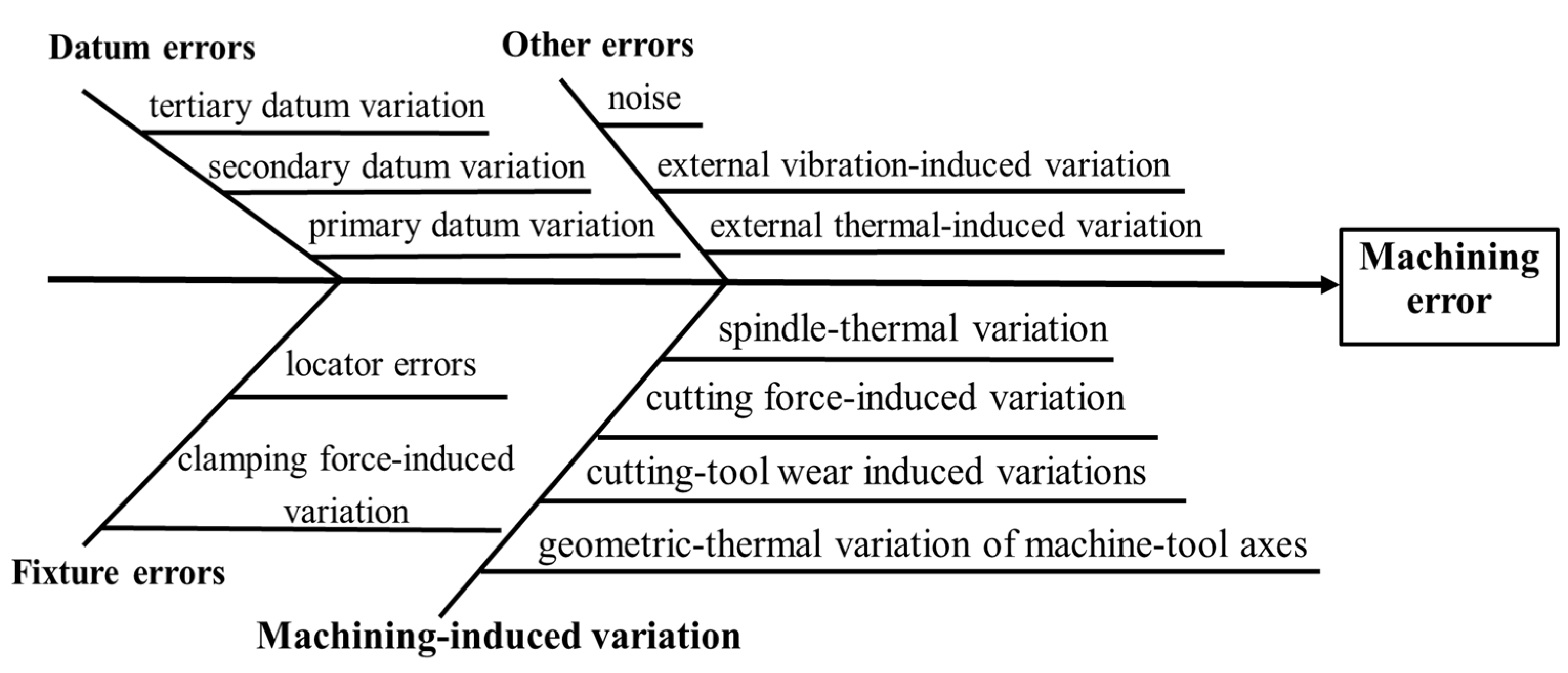
Figure 1. Ishikawa diagram of dimensional variation in machining processes.
Machines 11 00603 g001
Figure 2. Orthogonal 3-2-1 fixturing setup via a plane and three locators.
Machines 11 00603 g002
Figure 3. Non-orthogonal 3-2-1 fixture layout.
Machines 11 00603 g003
Figure 4. Steps of the derivation of variation propagation model for MMPs.
Machines 11 00603 g004
Figure 5. Top view of workpiece.
Machines 11 00603 g005
Figure 6. Workpiece and locating points.
Machines 11 00603 g006
Figure 7. Distance from feature 399 to hole C.
Machines 11 00603 g007
Figure 8. Distances from feature 399 to axis of hole C of 40 blocks.
Machines 11 00603 g008
Figure 9. Machining errors of 40 blocks.
Machines 11 00603 g009
Table 1. Nominal positions of locators in FCS.
Locator IndexDatum
Feature
Locator Coordinate in FCSOutgoing Normal
Direction
1A[40, 30, 100][0.4997, 0, 0.8662]
2A[70, 70, 80][0.4997, 0, 0.8662]
3A[110, 30, 40][0.4997, 0, 0.8662]
4B[−90, 0, 80][0, −1, 0]
5B[90, 0, 0][0, −1, 0]
6C[130, 50, −95][1, 0, 0]
Table 2. Nominal positions and orientations of features.
Feature Number t i R ω i R
A[0, 0, 110][0, 0.5233, 0]
B[45, 0, 0][π/2, 0, 0]
C[156, 40, −85][0, π/2, 0]
D[−130, 0, 20][0, −π – 0.8, 0]
Table 3. Variation sources and their variation values.
NumberVariation ValuesSources Description
1 0.040 0.045 0.023 0.0003 0 0 T Primary datum error
2 0.030 0.060 0.040 0.0002 0.0001 0 T Secondary datum error
3 0.010 0.020 0.050 0.0001 0.0001 0.0001 T Tertiary datum error
4 0 0 0 0 0 0 T Fixture error
5 0 0 0 0 0 0 T Machine tool path error
Table 4. Nominal positions of locators and orientations of the features in FCS.
Locator IndexCoordinateOrientationsFrom Feature
L1[−103, −182.75, 50.5][0, 0, 0]Primary datum feature
L2[81.5, −7.5, 50.5][0, 0, 0]
L3[97, −309.5, 50.5][0, 0, 0]
P1[−65, −312.5, 50.5][0, −π/2, 0]Secondary datum feature
P2[−111, −17, 50.5][0, −π/2, 0]
P3[−65, −312.5, 50.5][π/2, 0, 0]Tertiary datum feature
Table 5. Error sources and their corresponding values.
NumberVariation ValuesSources Description
1 0 0 0.01 0 0 . 0001 0 T Primary datum error
0.02 0.03 0.01 0 0 0 T Fixture error
Disclaimer/Publisher’s Note: The statements, opinions and data contained in all publications are solely those of the individual author(s) and contributor(s) and not of MDPI and/or the editor(s). MDPI and/or the editor(s) disclaim responsibility for any injury to people or property resulting from any ideas, methods, instructions or products referred to in the content.