Abstract
This research proposes a methodology for designing and testing a self-optimizing control (SOC) algorithm applied to a wind energy conversion system (WECS). The SOC maximizes WECS power output and reduces the mechanical stress of the wind turbine (WT) blades by optimizing a multiobjective cost function. The cost function computation uses a combined blade element momentum (BEM) and thin-wall beam (TWB) model for calculating wind the turbine power output and blades’ stress. The SOC deployment implies a low computational cost due to an optimization space reduction via a matrix projection applied to a measurement vector, based on a prior offline calculation of a projection matrix, . Furthermore, the SOC optimizes the operation of the WECS in the presence of uncertainty associated with the wind speed variation by controlling a linear combination of measured variables to a set point. A MATLAB simulation of a wind turbine model allows us to compare the WECS operating with the SOC, a baseline classic control system (BCS), and a nonlinear model predictive controller (NMPC). The SOC algorithm is evaluated in terms of power output, blades’ stress, and computational cost against the BCS and NMPC. The power output and blades’ stress performance of the SOC algorithm are compared with that of the BCS and NMPC, showing a significant improvement in both cases. The simulation results demonstrate that the proposed SOC can effectively optimize a WECS operation in real time with minimal computational costs.
1. Introduction
Wind power technology is a crucial element in all climate change mitigation strategies. Technological innovations and economies of scale have allowed the world wind energy market to grow considerably during the last decade. As a result, the installed capacity of wind energy grew to 837 GW at the end of 2021, contributing to an increased commercial demand for wind energy conversion systems (WECS) of all sizes [].
Wind turbines transform the kinetic energy contained in the wind into electric energy [,,]. Despite differences in structure, technology, and size, all wind turbines, from systems rated in the kW range to large systems with rated power values of several MW, are based on the same general principle [,,]. From a power system’s perspective, the most relevant distinction is based on the configuration for control and power conversion, with four basic types covering most commercially available products [,]. While a modern wind turbine has many control systems for different purposes [], the main control task is to regulate the power output as a function of the wind speed. Below the rated wind speed, the primary purpose of the control system is to deliver the maximum amount of power to the grid or (local) load at a given wind speed; this is generally referred to as maximum power point tracking (MPPT) [,]. When extracting power from the wind, wind turbines are exposed to several different loads, which have to be analyzed and accounted for in the design phase by a suitable structural design and material selection. Once put in operation, the stresses developing in the components of a wind turbine, particularly in the blades, are generally not monitored or controlled. However, structural health monitoring (SHM) systems are increasingly recognized in the academic literature [] as a requirement for very large wind turbines, particularly those operating in remote locations (such as offshore) where servicing operations are complex and costly.
1.1. Prior Work
Essential control functions in WT include active and passive stall regulation, and pitch angle control [,,]. While pitch control is generally used for output power control, it can be generalized to reduce the loads acting on the wind turbine blades, reducing the probability of fatigue damage. This approach was studied by Wu Hou Lio []. Modern control techniques such as nonlinear model predictive control (NMPC), adaptive model predictive control (AMPC), and proportional–integral–derivative schemes based on artificial neural networks (NN-PID) have been shown to be capable of reducing the stress levels in the blades for a given power extraction rate [,]. In an experimental set using a test-bench-mounted small-turbine generator coupled to a wind speed simulator, García et al. [] were able to show that even in a fixed blade setup, the combination of an advanced control scheme with an objective function considering both the extracted power and the blade stress allowed a reduction in the stress at a given output power level, or conversely, an increase in power for a given blade stress level. Loza et al. [] studied simulated fatigue damage in three small wind turbine configurations, using fixed-rpm (passive) stall control and blade-pitch control, both in a variable and a fixed-rpm configuration. The blade-pitch control generally allowed for a longer fatigue life, although the stall control did show some advantages at sites with high average wind speeds.
Similar work was conducted by Chenyang Yuan et al. [], who also developed a comparative study of the effect on fatigue life between a fixed-pitch and a blade-pitch control scheme, where the latter was based on a PID control system. The authors referred to the blade-pitch control as a baseline (classic) control system (BCS). Implementing the BCS resulted in a significant reduction in blade loads and a corresponding increase in fatigue life.
In [], a small signal model for a wind turbine equipped with a direct-drive permanent-magnet synchronous generator (PMSG) was presented, connected to the grid through power converters in a back-to-back configuration. The proposed small-signal model included two approaches: tip-speed ratio (TSR) control and optimum torque control (OTC). OTC was found to have superior performance and allowed for power output smoothing. The authors also claimed that mechanical stresses were reduced in the OTC control scheme.
A novel approach was proposed by Iordanov [] to explore the idea of “self-learning wind turbines.” A data-driven control scheme, termed self-optimizing control (SOC), was introduced and applied to a 5 MW offshore wind turbine. The focus of the work was on the maximization of power extraction. The proposed scheme was based on the measurements of the operating data of the wind power plant, such as power output (P), pitch angle (), angular speed, and torque of the rotor ( and , respectively), and the generator efficiency (). The objective was to determine an optimal control law by applying the so-called global SOC or gSOC scheme, which considered and as the manipulated variables, the wind speed (v) as the disturbance, and the objective function J to be maximized as the output power . The optimal control values were found through a regression and linear combination. The results indicated that the gSOC strategy successfully maximized J in region II of the WT without any prior knowledge of the dynamics of this relatively complex system but only based on the operational data provided.
1.2. Scope and Contribution
In the present work, the SOC control scheme proposed by Iordanov et al. [] was generalized to reconcile the conflicting objectives of minimizing mechanical stress in the WT blades and maximizing power extraction. The generalized SOC model draws on the previous work of two of the authors [,] on wind turbine control based on an aeroelastic model, which allows the calculation of high-resolution blade stress maps for any given operating point. Furthermore, defining a suitable objective function allows the co-optimization of the output power and blade stresses. It is shown that the modified SOC approach significantly reduces blades’ stresses for a given power output level compared to standard pitch control schemes, such as BCS. Additionally, the results are compared to those of a nonlinear model predicted control (NMPC) scheme.
The proposed SOC control scheme was implemented in MATLAB/Simulink. The simulations were conducted for various wind speeds and turbulence intensities, and the results were compared to those of the BCS and NMPC schemes. The comparison showed that the generalized SOC model outperformed BCS and NMPC regarding the blade stress reduction for a given power output level. Furthermore, it was also observed that the SOC control scheme could extract more power from the turbine compared to the NMPC while keeping blade stresses within acceptable levels. The results confirm that the generalized SOC model is an effective way to reconcile conflicting objectives in wind turbine operation.
Fatigue loading significantly affects wind turbines’ lifespan, especially in the rotor blades. Fatigue loading occurs due to the combination of the wind field’s stochastic nature impacting the rotor and rotational sampling caused by the finite spatial coherence of the wind field []. Excessive fatigue loads reduce blade life and increase maintenance costs and financial losses []. Therefore, a careful consideration of fatigue is crucial during wind turbine design and operation. Extensive literature exists on this subject, primarily focusing on utility-scale turbines due to the cost-effectiveness of testing. However, in small wind turbines, where manufacturers face challenges when conducting extensive testing, addressing fatigue becomes even more significant.
2. Wind Turbine Model
In this study a simulated phasor-type wind turbine model was implemented for which the SOC control scheme calculated an optimal value of the rotational speed of the WT , obtained from the minimization of a cost function combining the output power and the blade stress. This value, , minimized the cost function and ensured that the maximum power was extracted from the WECS while reducing the mechanical stress on the wind turbine blades. The normalized stress was calculated through an aeroelastic BEM/TWB model.
The wind turbine model was based on the configuration described in Rosyadi et al. []. Figure 1 shows the architecture of the wind turbine model, which is composed of a wind turbine rotor with pitch angle control, whose reference is the angular speed of the turbine; the drive train; a permanent-magnet synchronous generator (PMSG); a back-to-back electronic conversion system made up of the stator-side converter (SSC) and a grid-side converter (GSC), as well an LCL coupling filter. The GSC converts the dc voltage into a three-phase ac voltage with a fixed frequency, allowing for power injection into the grid. The PMSG and the LCL filter are modeled by voltage differential equations expressed in the dq reference system. Refer to Table 1 for a complete list of definitions of acronyms and variables used throughout this document.
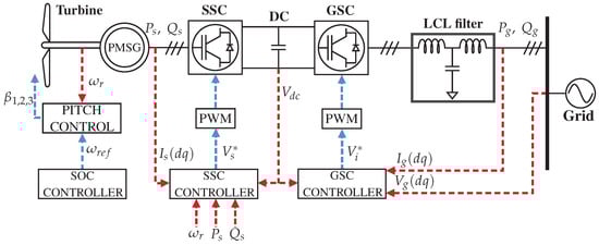
Figure 1.
Architecture of the phasor-type model for a WT based on PMSG.

Table 1.
Variables and acronyms definition.
2.1. Aerodynamic Model of the Wind Turbine
The aerodynamic model was based on a three-blade horizontal wind turbine model. The wind power that can be extracted from a WT can be written as follows:
where P is the power extracted from the wind, is the air density, A is the swept area for rotor radius R, is the wind speed, is the tip-speed ratio (TSR), is the pitch angle, is the rotational speed of the turbine shaft, and is the power coefficient, which is a function of both the tip speed and the pitch angle, . In [,] a parametric expression for is given as:
In this work, the coefficients of (3) given in [] were used: , , , , , and .
The power extraction characteristic as a function of the shaft rotational speed () for different wind speeds and a pitch angle of zero degrees is shown in Figure 2, which shows that for the nominal shaft frequency ( pu), the maximum power extraction is obtained at a wind speed of = 10 m/s.
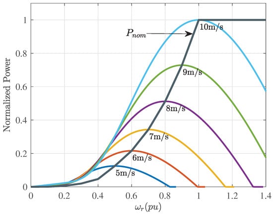
Figure 2.
Power and maximum power point (MPP).
The MPPT was calculated with (5). The advantage of using this relationship is that the wind speed is not measured directly, therefore variations in the wind are not instantly reflected in the reference signal. See [] for more details.
2.2. Integrated BEM/TWB Model
The BEM/TWB model formulation was taken from []. The BEM (blade element momentum) part of the model allows the calculation of blade loadings at different sections along the blade resulting from the aerodynamic lift and drag at each section, based on the calculated net inflow angle and the given lift and drag characteristics of the airfoil chosen for a given section [].
As opposed to traditional aeroelastic assessments of wind turbine blades, where the stress is typically monitored only at a fixed predefined location, the TWB model allows for the construction of a full stress map for the complete blade shell. Given the fast execution times, the BEM/TWB can be used in control applications where the use of detailed finite-element models would be prohibitive. The main assumptions in the model are listed below:
- The internal structure of the blade and the resonant effects produced by the wind are not considered;
- Aerodynamic forces are calculated using BEM theory in steady state;
- The rotor plane is always oriented perpendicular to the wind;
- The wind speed is uniformly distributed along the blade.
The axial and shear strains can be expressed as follows:
where is the axial strain on the surface along the axis (z), and is the shear strain in the plane of the blade material (s, z). Cartesian coordinates (x, y, z) are aligned with the movement in the flapwise, edgewise, and axial directions, respectively; n and s correspond to a system of normal and tangential coordinates of an arbitrary point located on the surface and with the origin located in the middle of the cross section; , , , and are the curvatures of the surface in the and planes, the twist rate, and the twist curvature, respectively; is the first-order axial stress on the axial line. contains coupling terms between axial strain and shear strain.
The blades of a wind turbine are manufactured with sheets that have a specific thickness, elastic properties, and different orientations (directional and bidirectional). From (6) and (7), it is possible to determine the axial () and shear () stress in the layer k at any position of the blade using a plane-stress orthogonal constitutive law []:
where are the stiffness coefficients of the material in the global coordinate system, which reduce to planar stress conditions through an orthotropic law.
The stresses of (8) are transformed to the material coordinate system using the rotation matrix [] as follows:
The TWB model calculates the stress value at each point in the shell of the wind turbine blade, allowing the most critical point on the blade to be determined at any given moment, as opposed to models where the stress is monitored only at a predetermined location (e.g., the root section of the blade). Criticality can be assessed by comparing the actual stress at a given location to the corresponding strength (), i.e., the maximum tolerable stress. This is done by defining the normalized stress factor () as
where (1,1) corresponds to stresses along the fiber directions, (2,2) to stresses perpendicular to the fiber, and (1,2) to shear stress.
The equations of motion for a section of a given aerodynamic profile at an axial position z in the blade can be expressed as
where , , and are the mass, stiffness, and hysteretic damping matrices, respectively, and
is the displacement vector at location z grouping the translational displacements in the x, y, and z directions, respectively, as well as the (elastic) rotational of the cross section around the z axis.
The forcing vector is given by
where represents the local loads acting on the blade segment due to the aerodynamic forces calculated by the BEM model, while , , and are the displacements, velocities, and accelerations of the blade section located at z, respectively. The angle of attack of the section is calculated as:
where is the flow angle determined by the blade element momentum (BEM) theory, is the (global) pitch angle, and is the rotation angle of the local blade section as determined by the geometry specified in the TWB model.
From Equation (10), it is possible to estimate the instantaneous normalized stress along the blade of the wind turbine. Figure 3 shows illustrative results of simulations conducted with the integrated BEM/TWB model summarized above. In the first case (Figure 3a), the wind turbine was operated with a fixed blade at a wind speed of 9.4925 m/s to illustrate the stress distribution at a blade of a stall-regulated wind turbine (see [] for typical operational characteristics). High-stress levels (relative to the specified material strength values) can occur near the root section but are not limited to it, as demonstrated by the continuous band of high relative stress extending to the midsection of the blade. As illustrated in Figure 3b, where the stress map for a pitch-regulated wind turbine operating at the same wind speed of 9.4925 m/s is shown, the blade-pitch regulation allows a notable reduction in stress.
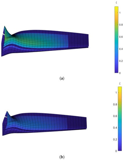
Figure 3.
Airfoil with different stress levels calculated with the BEM/TWB model. The simulation result was obtained in MATLAB with a computational time of 5.77 s. (a) Relative stress map for the wind turbine operating with a stall regulation at a wind speed of 9.4925 m/s. (b) Relative stress map for the wind turbine operating with a pitch regulation at a wind speed of 9.4925 m/s.
3. Self-Optimizing Controller
Self-optimizing control automatically adjusts the controller parameters to optimize system performance without external intervention. This control algorithm continuously analyzes the system it controls through feedback and adjusts its settings to improve its performance. Furthermore, it applies optimization algorithms to adjust the control parameters in real time to achieve optimal performance even in dynamic or unpredictable environments.
Since this work compares SOC with an NMPC, some distinctions are made. Self-optimizing and predictive control are two different approaches to controlling complex systems. While both methods involve optimizing control parameters, there are some critical differences between them, as follows:
- Feedback vs. feed-forward: Self-optimizing control is a feedback-based approach where the control system continuously monitors the process output and adjusts the control input based on the feedback. On the other hand, predictive control is a feed-forward-based approach that predicts future outputs based on the system’s current state and adjusts the control input accordingly.
- Model-based vs. model-free: Predictive control requires a mathematical model of the system being controlled to predict the future behavior of the system. Self-optimizing control does not require a model of the system and relies on data-driven optimization techniques to adjust the control parameters.
- Reactive vs. proactive: Self-optimizing control is a reactive approach that responds to changes in the system in real time. Moreover, predictive control is a proactive approach that anticipates changes in the system and adjusts the control input accordingly.
- Adaptability: Self-optimizing control is designed to adapt to changes in the system over time and can continuously optimize the control parameters. On the other hand, predictive control requires a new model to be developed if there are significant changes in the system.
Figure 4 shows the block diagram of the proposed adaptation of the SOC control scheme for controlling a wind turbine. The control architecture operates on the wind turbine as a supervisor of the phasor-type model shown in Figure 1. The objective is to find the optimal value of the controlled variable, , whose value is the set point for the pitch angle controller . Figure 5 shows the traditional pitch control scheme (included in the BCS architecture), which includes the variable calculated from the SOC to further adjust accordingly. The reference is the normalized speed in pu (per unit) of the generator. This controller is activated with wind speeds greater than the nominal (). For speeds below nominal, .
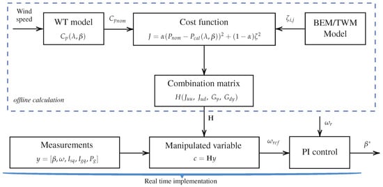
Figure 4.
Architecture of the control scheme SOC.
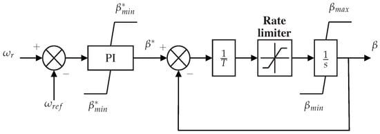
Figure 5.
Pitch controller.
3.1. Cost Function
The objective was to maximize power extraction while minimizing stress on the turbine blades. The cost function considered the power and stress factor through a combination of these variables as follows:
where is the nominal power, is the calculated power, is the maximum stress of (10) calculated along the blade, and is an optimization parameter whose value is calculated in accordance with a Pareto front analysis.
The cost function combined the power output and stress variables to create a trade-off between the two. The cost function was designed to maximize power extraction while minimizing stress on the turbine blades. This cost function was used to evaluate the performance of the control strategies and determine which one was the most suitable for a given wind energy conversion system (WECS).
Different techniques have been developed to solve multiobjective optimization problems. One of the most widely used techniques for determining the Pareto front is by considering individual objectives separately. The weighted sum approach involves selecting weights and calculating a linear combination of the different goals:
Because the weighted sum approach uses a convex combination of objectives, multiple optimization realizations are required to approximate the Pareto optimal set []. Figure 6 shows the feasible solutions achieved by evaluating the self-optimized control scheme’s cost function, Equation (15), with different weighting values . In this context, the Pareto front is represented as the maximum value of the stress factor and the power of the baseline control (BCS). As the weight value () decreases, the feasible solutions tend to the maximum stress and power of the baseline control. The closest to the Pareto optimal solution is achieved with .
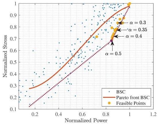
Figure 6.
Pareto front with feasible solutions.
3.2. Combination Matrix
The variables and equations of interest involved in the SOC control structure, according to [,,,], are:
- : (manipulated variables) “base set” for unconstrained degrees of freedom.
- : disturbance or set of disturbances.
- : optimal value of u for a given disturbance d.
- : objective cost function.
- : set-points.
- : implementation error or measurement error.
- : true measurements (without ).
- : measurements at the process output (with ).
- : optimal projection matrix of selection or combination of measurements.
- : selected controlled variables.
- : optimal value of c for a given disturbance d.
The architecture of the SOC control requires determining a combination matrix of the system measurements, , to determine the control variables from the process measurements []:
To determine , it is first necessary to find the Hessian matrix , given by Equation (18):
where:
- ;
- ;
- ;
- .
The optimal sensitivity matrix can then be determined, which is calculated using the matrix of the gains of each input (measurement) , and the matrix of the gains of each measurement before each disturbance , through Equation (19):
Using the diagonal matrix of perturbations , and the diagonal matrix of measurement errors (noise) , one can find ,
The combination matrix, , can be found as follows []:
For the wind turbine control system, the manipulated variable (), measurements (), and disturbance () are defined as:
where is the angular velocity of the generator, is the pitch angle, is the quadrature current of the generator, is the current in the grid quadrature, is the active power in the grid, and is the normalized stress calculated by the BEM/TWB model. As shown in Equation (15), the disturbances are directly related to the cost function, so the optimization was performed for each value of the wind series used in this study.
The values of the diagonal matrices, and of (20), were chosen after performing several experiments in which it was verified that they held the individual objectives of the cost function (15). The wind series used () contained pu values in the range of , the best results were achieved when considering
and the instrumentation error for was 4.5%; , , , and were 1% and was 3.5%.
3.2.1. Gain Matrix
The gain matrix, , was obtained by evaluating the indirect manipulated variable () around the nominally optimal operating point. Gain values were obtained for each measurement by using finite differences. The calculation of finite differences was carried out on interpolation polynomials that could represent experimental data. This presents an advantage when the real functionality of the data to be represented through concrete functions has yet to be discovered exactly []. The derivative of five points was used, which was obtained by interpolating the points , , and , where the separation h was constant. Equation (25) shows the expression for approximating the derivative at a point where .
The results obtained in [] were used in this study to calculate the gain matrix by evaluating the manipulated variable near the nominal value that corresponds to the region where the generator is kept at constant speed. The value of with was experimentally defined. It is important to mention that this process must be carried out for each of the measurements of y. Figure 7 shows the graph of the behavior of the pitch angle versus the rotational speed ().
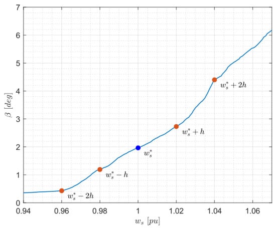
Figure 7.
Evaluation points to obtain the profit .
After calculating the gain values for the measurements, the following results were obtained:
After calculating the finite derivatives, the value of the gain corresponding to each individual measurement can be determined by:
The matrix of gains against disturbances was calculated with the same logic. Figure 8 shows the behavior of the step angle against the disturbance () together with the evaluation points. The nominal value of the normalized disturbance was defined as , which corresponded to the wind speed where the maximum power was achieved (10 m/s).
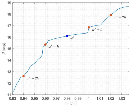
Figure 8.
Evaluation points to obtain the profit .
3.2.2. Hessian Matrix Calculation
The Hessian matrix was obtained around the nominally optimal point:
By using the symbolic tools of Matlab, the Hessian matrix was calculated as: (hessian(J, [w, v])), where J is the cost function, Equation (15), as a function of the symbolic variables, w and v, which represent the controlled variable () and the disturbance (), respectively.
3.3. SOC Algorithm
This subsection presents the self-optimized control algorithm implemented on the simulated model of the wind turbine. It was necessary to initialize the value of the optimization parameter, , and the diagonal matrices of the expected value of the perturbation and implementation error, and , respectively. Then, the variables corresponding to the vectors of the manipulated variable (), measurements (), and disturbances () were obtained. Then, the cost function (J) was defined and the Hessians ( and ) were calculated. With this, it was possible to calculate the combination matrix, , and then proceed to calculate the controlled variable defined as the angular velocity of the generator () that enters the pitch angle control system. Steps 4 and 5 repeat indefinitely, while the rest of the algorithm is executed once to calculate . Please see details in Algorithm 1.
| Algorithm 1 SOC algorithm. |
| 1. Obtains the vector input, measurements and disturbance: |
| 2. Define cost function: |
| 3. Combination Matrix: |
| 4. Controller variable: |
| 5. Define: |
4. Results and Discussion
The results were obtained using the SOC control scheme on a phasor-type wind turbine model based on a permanent-magnet synchronous generator. The simulation was implemented in Matlab/Simulink using the parameters listed in Table A1 of Appendix A. The performance obtained by applying the SOC scheme for different operating conditions was compared with two other control schemes, NMPC and BCS.
Comparison of Results between Referential Control Schemes
A brief explanation of the objectives of the control schemes used for the comparison is presented below:
- The baseline control scheme (BCS) offers power control in the third zone (region III) of the operation of the wind turbine and torque control for the maximum power point tracking in the second zone (region II) of operation.
- Nonlinear model predictive control (NMPC) seeks optimal operational points in the controlled variables and . The former variable is calculated exclusively for wind speeds below the nominal value (region II).
- Self optimizing control (SOC) performs power and torque control in the WT’s third operating zone. is calculated to maximize the inverse relationship between the extracted power and the stress factor. SOC constitutes a gentle update on the architecture of the BCS.
The wind speed time series used in the simulation is shown in Figure 9. The red line indicates the nominal value of the wind speed (10 m/s). This time series was generated with Turbsim, and the wind series had a mean speed value of 9.32 m/s. When the wind speed exceeded the nominal value, the angular speed of the rotor was regulated by the manipulated variable . It can be seen that is zero in the region where the wind speed is below the nominal value, while changes its value when the wind speed exceeds the rated value.
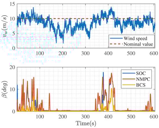
Figure 9.
behavior for the SOC, NMPC, and BCS control schemes.
Figure 10 shows a graphical comparison of the time series of the output power and the stress of the WECS when operating with the three control schemes. The maximum power, as expected, was obtained with the BCS, and the maximum stress levels during the simulation also occurred with this baseline control scheme. The NMPC and the SOC exhibited a power curtailment during the test, which was a trade-off for reducing the stress over the blades. Stress reduction can be seen to be quite significant (Figure 10). The results of this experiment show that the BCS provides the highest power output, but it also increases stress on the blades. On the other hand, NMPC and SOC can reduce this stress significantly while still providing a reasonable amount of power. This is especially beneficial for the long-term operation of WECSs, since it helps protect them from wear and tear. Moreover, since these two control schemes can provide a stable output with fewer variations, they can be used effectively to increase the lifetime of WECSs.
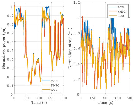
Figure 10.
Time-series comparison of the normalized power and the stress for the three control schemes.
The results in Figure 11 further reinforce the conclusion that the SOC scheme is the best choice for this system. Not only does it have a higher average power output than the reference controllers, but its variance is also significantly lower. This suggests that it produces more consistent results over multiple trials, making it an attractive option for applications where reliability is of paramount importance. More importantly, its stress factor results are much lower than either of the reference controllers, making it a safe and reliable choice for this system.
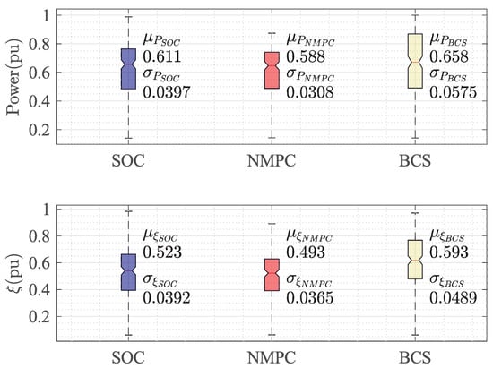
Figure 11.
Comparison between power output and stress factor.
Figure 12 shows a graphical comparison of the normalized power output of the WECS at specific stress levels when operating with the three different control schemes (SOC, NMPC, and BCS). Unsurprisingly, the BCS reaches the maximum power extraction since its control objective only considers power maximization. However, the stress level is much greater than the ones achieved by either NMPC or SOC, as demonstrated by the displacement of the heavy blue line (average power–stress relation for BCS) to the right of the black (SOC) and the red (NMPC) lines. The SOC performance is consistently better than that of NMPC, i.e., the average SOC operating values in the power–stress plane always dominate the average NMPC solutions (in a Pareto sense), although not by a large margin. The advantage over the BCS method is much more evident since the average SOC solutions dominate the BCS solutions by large margins, except for high power values where, by definition, BCS tends to dominate on the power axis. However, the BCS does not provide any stress relief to the turbine blades. As a result, the wind turbine’s power output can suffer in long-term scenarios due to fatigue and other issues. It is therefore essential to consider the effects of stress when selecting a control strategy for a wind energy conversion system. The results presented in Figure 12 indicate that while BCS may provide a higher power output in short-term scenarios, it may not be optimal for long-term operation. SOC and NMPC are more suitable for prolonged operation as they offer stress relief at a small energy penalty.
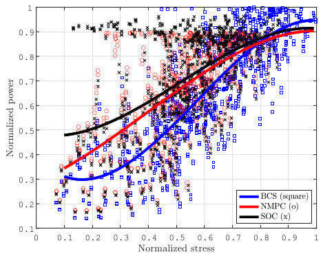
Figure 12.
Comparison of the power extracted from the wind turbine at a specific stress level with the three control schemes.
In addition, the SOC control scheme is computationally inexpensive compared to the BCS and NMPC schemes. In terms of computational cost, the SOC algorithm requires significantly fewer time steps and is more computationally efficient than the NMPC. This makes it an ideal choice for real-time optimization of a WECS since it can achieve a good balance between power output and blades stress while keeping computational costs low. Furthermore, the SOC algorithm can be easily implemented in existing WECS control systems with minimal modifications. This makes it a viable option for wind turbine owners who are looking to optimize their WECS in real time without incurring significant additional costs.
The power curtailment of the SOC and NMPC controllers over the BCS was calculated as:
The SOC and NMPC control schemes reduced the power output compared to the BCS ( power curtailment) control by and , respectively. This power reduction corresponded to the variation in rotational speed (Figure 10), . Similarly, the percentage of stress reduction using the SOC and NMPC control schemes versus the BSC can be calculated as:
The SOC and the NMPC reduced the stress factor, , by and , respectively. Table 2 shows the results for the control schemes (NMPC and SOC) in comparison with the BSC scheme for different wind speeds and turbulence intensities. Regarding the SOC control scheme, a reduction of the stress factor of about 18% was achieved. This result corresponded to the power reduction above .
Table 2.
Summary of operating results for the different control schemes.
The normalized PSD calculated for each of the control schemes, SOC, NMPC, and BCS, is shown in Figure 13. Figure 13a,b show the results for the power fluctuations and the stress factor, respectively, demonstrating that the implementation of the SOC achieved a decrease in both power fluctuations and stress spectral components.
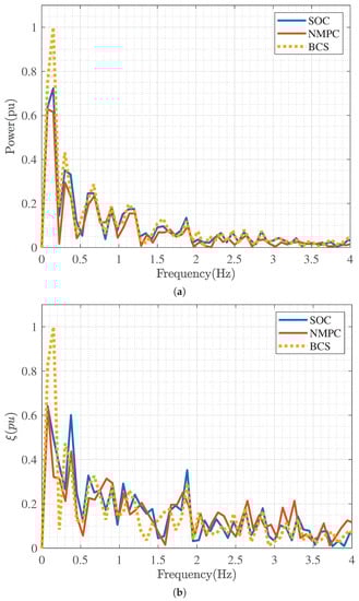
Figure 13.
Comparison of the response in frequency of the behavior of the controllers using the PSD. (a) PSD of the output power. (b) PSD of the stress factor, .
Table 3 shows the computation time for each control scheme. It can be noticed that the processing time of the SOC control scheme was significantly shorter than for NMPC under identical simulation conditions; in this case, this implied a wind speed time series with a duration of 605 s. The simulations were carried out on a personal computer with an Intel Core i7-7700HQ CPU @2.80 GHz and 16 GB of RAM.
Table 3.
Computation time of each control scheme.
5. Conclusions
In the present work, a novel control scheme was introduced, allowing for the efficient co-optimization of output power and blade stresses. The work built on a recently proposed self-optimization control (SOC) for wind turbines and prior work of two of the authors on the efficient modeling of blade stress. The proposed novel control scheme allows for a notable reduction in blade stress at a modest energy penalty, i.e., a curtailment of output power. Apart from this favorable trade-off, the SOC also significantly reduced the fluctuations of both the power output and average blade stress. Both reductions are additional achievements which translate into important benefits: reductions in power output fluctuation diminish intermittency and make the turbine more grid-friendly; a lower stress fluctuation level, on the other hand, translates into fewer fatigue cycles (which also have smaller amplitudes) and therefore a longer fatigue life of the turbine blades.
The proposed SOC strategy significantly outperformed a reference strategy, termed BCS, modeled after the standard operation of commercial wind turbines, as well as a nonlinear model predicted control (NMPC) scheme. While the BCS strategy did not explicitly consider stress as part of the control objectives, the NMPC scheme did work on the same combined objective function as the SOC approach; therefore, the superior performance of the novel (SOC) was not anticipated from the outset. The work did confirm the initial expectation that the SOC would be more computationally efficient than the NMPC method. This finding paves the way for a real-time implementation of the proposed method in commercial wind turbines.
Author Contributions
Conceptualization, L.I.M. and O.P.; methodology, L.I.M. and O.P.; software, C.E.R. and G.D.M.; validation, L.I.M. and O.P.; formal analysis, L.I.M. and O.P.; investigation, C.E.R. and G.D.M.; resources, L.I.M.; data curation, C.E.R.; writing—original draft preparation, C.E.R. and G.D.M.; writing—review and editing, L.I.M. and O.P.; supervision, L.I.M. All authors have read and agreed to the published version of the manuscript.
Funding
This research received no external funding.
Data Availability Statement
No new data were created or analyzed in this study. Data sharing is not applicable to this article.
Acknowledgments
This work did not receive any direct funding. However, it did build on earlier work funded by CONACYT/Fondo de Sostenibilidad Energética through the Mexican Center for Innovation in Wind Energy (CEMIE Eólico) for project P19 (reliability of small wind turbines).
Conflicts of Interest
The authors declare no conflict of interest.
Appendix A
Simulation Parameters
The WECS, WT, and PMSG parameters used in the simulation are shown in Table A1. Some variables are normalized to (per unit) values.
Table A1.
Simulation parameters.
Table A1.
Simulation parameters.
| Parameter | Value |
|---|---|
| Rated power | 1.5 MW |
| Rated voltage | 1.8 kV |
| Rated frequency | 60 Hz |
| Stator resistance | 0.022 pu |
| Stator direct axis inductance | 1.2 pu |
| Stator quadrature axis inductance | 0.71 pu |
| Permanent magnet flux | 1.3 pu |
| Turbine constant of inertia | 3.5 s |
| Generator inertia constant | 0.9 s |
| Turbine damping | 1.5 |
| Spring constant | 296 |
| Inverter-side inductance | 82.4 H |
| Parasitic resistance of | 3.6 |
| Grid-side inductance | 16.5 H |
| Parasitic resistance of | 1 |
| Filter capacitor | 122 H |
| Damping resistance | 0.05 |
| Air density () | 1.1839 kg/m |
| Rotor blade radius (R) | 3.4 m |
| Optimal TSR | 8.1 |
| Optimal power coefficient | 0.48 |
References
- GWEC. Global Wind Report 2021. 2021. Available online: https://gwec.net/global-wind-report-2021/ (accessed on 20 December 2021).
- Wu, B.; Lang, Y.; Zargari, N.; Kouro, S. Power Conversion and Control of Wind Energy Systems, 1st ed.; IEEE Press Series on Power Engineering; Wiley-IEEE Press: Hoboken, NJ, USA, 2011; ISBN 9780470593653. [Google Scholar]
- Heier, S. Grid Integration of Wind Energy, Onshore and Offshore Conversion Systems, 3rd ed.; John Wiley & Sons, Ltd.: Hoboken, NJ, USA, 2014; Chapter 2; pp. 31–117. ISBN 9781118703274. [Google Scholar] [CrossRef]
- Söder, L.; Ackermann, T. Wind Power in Power Systems: An Introduction. In Wind Power in Power Systems, 1st ed.; Ackermann, T., Ed.; Electric Power Systems; John Wiley & Sons, Ltd.: Hoboken, NJ, USA, 2005; Chapter 3; pp. 25–51. [Google Scholar] [CrossRef]
- Rojas Maita, C.P. Evaluación de los Recursos Eólicos para la Generación de Energía Eléctrica a Pequeña Escala en el Distrito de Huachac. Master’s Thesis, Universidad Nacional del Centro del Perú (UNCP), Huancayo, Peru, 2020. [Google Scholar]
- Ackermann, T. Historical Development and Current Status of Wind Power. In Wind Power in Power Systems, 1st ed.; Ackermann, T., Ed.; Electric Power Systems; John Wiley & Sons, Ltd.: Hoboken, NJ, USA, 2005; Chapter 2; pp. 7–24. [Google Scholar] [CrossRef]
- Rayyan Fazal, M. Wind energy. In Renewable Energy Conversion Systems; Kamran, M., Rayyan Fazal, M., Eds.; Academic Press: Cambridge, MA, USA, 2021; Chapter 5; pp. 153–192. [Google Scholar] [CrossRef]
- Pao, L.Y.; Johnson, K.E. Control of Wind Turbines: Approaches, Challenges, and Recent Developments. IEEE Control Syst. Mag. 2011, 31, 44–62. [Google Scholar] [CrossRef]
- Johnson, K.; Pao, L.; Balas, M.; Fingersh, L. Control of Variable-Speed Wind Turbines: Standard and Adaptive Techniques for Maximizing Energy Capture. IEEE Control Syst. Mag. 2006, 26, 70–81. [Google Scholar] [CrossRef]
- Bianchi, F.D.; Battista, H.D.; Mantz, R.J. Wind Turbine Control Systems Principles, Model and Gain Scheduling Design, 1st ed.; Advances in Industrial Control; Springer: Berlin/Heidelberg, Germany, 2007; pp. 7–69. ISBN 9781849966115. [Google Scholar]
- Abdullah, M.; Yatim, A.; Tan, C.; Saidur, R. A review of maximum power point tracking algorithms for wind energy systems. Renew. Sustain. Energy Rev. 2012, 16, 3220–3227. [Google Scholar] [CrossRef]
- Kot, R.; Rolak, M.; Malinowski, M. Comparison of maximum peak power tracking algorithms for a small wind turbine. Math. Comput. Simul. 2013, 91, 29–40. [Google Scholar] [CrossRef]
- Martinez-Luengo, M.; Kolios, A.; Wang, L. Structural health monitoring of offshore wind turbines: A review through the Statistical Pattern Recognition Paradigm. Renew. Sustain. Energy Rev. 2016, 64, 91–105. [Google Scholar] [CrossRef]
- Lio, W.H.A. Blade-Pitch Control for Wind Turbine Load Reductions, 1st ed.; Springer: Cham, Switzerland, 2018; p. 174. [Google Scholar] [CrossRef]
- Minchala, I.; Probst, O.; Cárdenas, D. Wind turbine predictive control focused on the alleviation of mechanical stress over the blades. IFAC-PapersOnLine 2018, 51, 149–154. [Google Scholar] [CrossRef]
- Mínchala, L.I.; Cárdenas-Fuentes, D.; Probst, O. Control of mechanical loads in wind turbines using an integrated aeroelastic model. In Proceedings of the 2017 IEEE PES Innovative Smart Grid Technologies Conference—Latin America (ISGT Latin America), Quito, Ecuador, 20–22 September 2017; pp. 1–6. [Google Scholar] [CrossRef]
- Garcia, M.; San-Martin, J.; Favela-Contreras, A.; Minchala, I.; Cárdenas, D.; Probst, O. A Simple Approach to Predictive Control for Small Wind Turbines with an Application to Stress Alleviation. Control Eng. Appl. Inform. 2018, 20, 69–77. [Google Scholar]
- Loza, B.; Pacheco-Chérrez, J.; Cárdenas, D.; Minchala, L.I.; Probst, O. Comparative Fatigue Life Assessment of Wind Turbine Blades Operating with Different Regulation Schemes. Appl. Sci. 2019, 9, 4632. [Google Scholar] [CrossRef]
- Yuan, C.; Li, J.; Xie, Y.; Bai, W.; Wang, J. Investigation on the Effect of the Baseline Control System on Dynamic and Fatigue Characteristics of Modern Wind Turbines. Appl. Sci. 2022, 12, 2968. [Google Scholar] [CrossRef]
- Nasiri, M.; Milimonfared, J.; Fathi, S. Modeling, analysis and comparison of TSR and OTC methods for MPPT and power smoothing in permanent magnet synchronous generator-based wind turbines. Energy Convers. Manag. 2014, 86, 892–900. [Google Scholar] [CrossRef]
- Gueorguiev Iordanov, S.; Collu, M.; Cao, Y. Can a Wind Turbine Learn to Operate Itself? Evaluation of the potential of a heuristic, data-driven self-optimizing control system for a 5 MW offshore wind turbine. Energy Procedia 2017, 137, 26–37. [Google Scholar] [CrossRef]
- Burlibaşa, A.; Ceangă, E. Rotationally sampled spectrum approach for simulation of wind speed turbulence in large wind turbines. Appl. Energy 2013, 111, 624–635. [Google Scholar] [CrossRef]
- Yang, W.; Peng, Z.; Wei, K.; Tian, W. Structural Health Monitoring of Composite Wind Turbine Blades: Challenges, Issues and Potential Solutions. IET Renew. Power Gener. 2017, 11, 411–416. Available online: https://eprints.ncl.ac.uk (accessed on 22 August 2022). [CrossRef]
- Rosyadi, M.; Umemura, A.; Takahashi, R.; Tamura, J.; Kondo, S.; Ide, K. Development of phasor type model of PMSG based wind farm for dynamic simulation analysis. In Proceedings of the 2015 IEEE Eindhoven PowerTech, Eindhoven, The Netherlands, 29 June–2 July 2015; pp. 1–6. [Google Scholar] [CrossRef]
- Carpintero Renteria, M.; Santos-Martin, D.; Lent, A.; Ramos, C. Wind turbine power coefficient models based on neural networks and polynomial fitting. IET Renew. Power Gener. 2020, 14, 1841–1849. [Google Scholar] [CrossRef]
- González, J.; Salas, R. Representation and estimation of the power coefficient in wind energy conversion systems. Rev. Fac. Ing. Uptc 2019, 28, 77–90. [Google Scholar] [CrossRef]
- Parikshit, G.; Jamdade; Santosh, V.P.; Vishal, B.P. Assessment of Power Coefficient of an Offline Wind Turbine Generator System. Int. J. Eng. Res. Technol. (IJERT) 2013, 2, 41–48. [Google Scholar]
- Cárdenas, D.; Escárpita, A.A.; Elizalde, H.; Aguirre, J.J.; Ahuett, H.; Marzocca, P.; Probst, O. Numerical validation of a finite element thin-walled beam model of a composite wind turbine blade. Wind Energy 2012, 15, 203–223. [Google Scholar] [CrossRef]
- Purcell, E.M. Life at low Reynolds number. Am. J. Phys. 1977, 45, 3–11. [Google Scholar] [CrossRef]
- Smith, S.; Southerby, M.; Setiniyaz, S.; Apsimon, R.; Burt, G. Multiobjective optimization and Pareto front visualization techniques applied to normal conducting rf accelerating structures. Phys. Rev. Accel. Beams 2022, 25, 062002. [Google Scholar] [CrossRef]
- Jaschke, J.; Cao, Y.; Kariwala, V. Self-optimizing control? A survey. Annu. Rev. Control 2017, 43, 199–223. [Google Scholar] [CrossRef]
- Alstad, V.; Skogestad, S.; Hori, E.S. Optimal measurement combinations as controlled variables. J. Process Control 2009, 19, 138–148. [Google Scholar] [CrossRef]
- Halvorsen, I.J.; Skogestad, S.; Morud, J.C.; Alstad, V. Optimal Selection of Controlled Variables. Process Des. Control 2003, 42, 3273–3284. [Google Scholar] [CrossRef]
- Kariwala, V.; Cao, Y.; Janardhanan, S. Optimal measurement combinations as controlled variables. IFAC Proc. Vol. 2007, 40, 257–262. [Google Scholar] [CrossRef]
- Dunn, S.M.; Constantinides, A.; Moghe, P.V. Finite Difference Methods, Interpolation and Integration. In Numerical Methods in Biomedical Engineering; Dunn, S.M., Constantinides, A., Moghe, P.V., Eds.; Biomedical Engineering; Academic Press: Burlington, NJ, USA, 2006; Chapter 6; pp. 163–208. [Google Scholar] [CrossRef]
Disclaimer/Publisher’s Note: The statements, opinions and data contained in all publications are solely those of the individual author(s) and contributor(s) and not of MDPI and/or the editor(s). MDPI and/or the editor(s) disclaim responsibility for any injury to people or property resulting from any ideas, methods, instructions or products referred to in the content. |
© 2023 by the authors. Licensee MDPI, Basel, Switzerland. This article is an open access article distributed under the terms and conditions of the Creative Commons Attribution (CC BY) license (https://creativecommons.org/licenses/by/4.0/).