Abstract
Point clouds represent an important way for robots to perceive their environments, and can be acquired by mobile robots with LiDAR sensors or underwater robots with sonar sensors. Hence, real-time semantic segmentation of point clouds with onboard edge devices is essential for robots to apprehend their surroundings. In this paper, we propose an onboard point cloud semantic segmentation system for robotic platforms to overcome the conflict between attaining high accuracy of segmentation results and the limited available computational resources of onboard devices. Our system takes raw a sequence of point clouds as inputs, and outputs semantic segmentation results for each frame as well as a reconstructed semantic map of the environment. At the core of our system is the transformer-based hierarchical feature extraction module and fusion module. The two modules are implemented with sparse tensor technologies to speed up inference. The predictions are accumulated according to Bayes rules to generate a global semantic map. Experimental results on the SemanticKITTI dataset show that our system achieves +2.2% mIoU and 18× speed improvements compared with SOTA methods. Our system is able to process 2.2 M points per second on Jetson AGX Xavier (NVIDIA, Santa Clara, USA), demonstrating its applicability to various robotic platforms.
1. Introduction
A point cloud is a set of 2D or 3D points, describing the geometric characteristics of objects in a scene. With the development of sensor technology, it has become more and more convenient for robots to collect point clouds from the environment [1]. For example, ground mobile robots can collect a 3D point cloud through LiDAR (light detection and ranging) devices; and underwater robots can use sonar devices to acquire a 2D point cloud of the sea environment. Hence, from both an academic and industrial perspective, point-cloud-based scene perception has attracted great attention [2,3].
Despite the tremendous potential of point cloud semantic segmentation, it faces significant challenges that must be addressed to make it practical for real-world applications. One of the primary issues is the high computational cost required to process and analyze large volumes of point cloud data. This limitation makes it hard to deploy point cloud segmentation systems on resource-constrained devices, especially for robotic platforms with edge devices.
Existing methods for semantic segmentation of point clouds consist of three categories: point-based methods, multi-view-based methods, and voxel-based methods. Each of the three semantic segmentation methods has its own set of advantages and disadvantages. The original point-based methods [4,5] are effective for segmenting large outdoor scenes but are computationally inefficient. On the other hand, the multi-view-based methods [6,7] are computationally efficient but can result in information loss and reduced segmentation accuracy when projecting 3D structures into 2D. Meanwhile, the voxel-based methods [8,9] perform better in 3D data, but dense convolutional neural networks are less efficient due to sparsity. While combining this method with sparse operations can improve efficiency, existing methods still cannot meet both efficiency and accuracy requirements simultaneously.
To realize real-time prediction for devices such as robots, we propose a real-time semantic segmentation system for point clouds based on use of a transformer and sparse convolution (TSR-Net). Firstly, we pre-process the data collected by LiDAR to obtain 3D data based on the sparse tensor. Next, we propose a sparse convolutional neural network involving two parts: feature extraction and fusion. To improve the ability of the network to learn global semantic features, we present a global feature extraction module (GFEM) in the feature extraction section. The GFEM helps to capture global semantic information from the point cloud data to improve the precision and accuracy of the segmentation results. Additionally, we introduce a channel attention module (CAM) in the feature fusion section to fuse different levels of semantic features, further enhancing the accuracy of the segmentation results. Finally, we obtain local segmentation maps by post-processing the data and further construct a global semantic map. Our main contributions are:
- (1)
- We propose a real-time semantic segmentation system of point clouds for robotic platforms to achieve both high accuracy and high efficiency with limited computational onboard devices. Our system outputs predictions for each point cloud and a reconstructed global semantic map.
- (2)
- We present a global feature extraction module and a channel attention module based on a transformer for hierarchical feature extraction and fusion. The two modules are lightweight in design and implemented with spare representations to speed up the inference time.
- (3)
- Experimental results show that our system outperforms existing state-of-the-art methods on the SemanticKITTI dataset by 2.2% mIoU (mean intersection over union) and 18× speedup. It can process 2.2 million points per second on NVIDIA Jetson AGX Xavier, demonstrating its applicability to a variety of robotic platforms.
2. Related Work
Existing semantic segmentation of point cloud methods fall into the following three main categories:
Raw point-based methods usually learn features directly from unordered point cloud data, such as STPC [4], and PAConv [5]. In particular, PAConv’s convolution kernel is a combination of multiple weight matrices. During the process, the coefficients of these weights are obtained by adaptive learning of the location relationships of the points. This data-driven approach to constructing convolutional kernels gives PAConv great flexibility to deal better directly with the point cloud data.
Multi-view-based methods typically involve projecting 3D data onto 2D images [10] and processing them using convolutional operations, as seen in PolarNet [6] and SqueezeSegV3 [7]. To address the problem of different feature distributions at different locations in the LIDAR images, SqueezeSegV3 proposes a spatially adaptive convolutional technique that adjusts the weights based on the input and location within the image.
Voxelization-based methods convert point cloud data into a dense grid and use 3D convolution for processing. Several methods have been developed to improve the computational efficiency of dense convolution, such as SPVNAS [8], Minkowski-Net [9], and MVASPP [11]. Minkowski-Net handles high-dimensional data by employing generalized sparse convolution and 4D spatio-temporal convolution. On the other hand, MV-ASPP extends PolarNet by using a pyramidal structured network to combine feature information at multiple scales and an ASPP module to expand the perception field.
The above is a division based on different representations of the data. In order to decrease the computational effort of the rasterization method, we introduce a sparse tensor into the system. Sparse convolution is a powerful technique utilized in some deep learning models to reduce the computational effort of point cloud data processing by performing convolutions only on non-empty regions. This technique reduces the computation quantity by computing convolutions only on the effective raster. Models such as Latticenet [12] and Cylinder3d [13] have successfully implemented sparse convolution. In particular, Cylinder3d is a 3D object detection model that uses sparse convolution and a columnar segmentation network to improve the prediction accuracy for objects such as vehicles and pedestrians, by leveraging an asymmetric residual module.
To increase the segmentation accuracy, we introduced the transformer module into the system. The transformer architecture, based on the self-attentive mechanism, has yielded great results in language processing (NLP). By abandoning convolutional operations and capturing global dependencies in the input sequence through attention only, this architecture is highly scalable. Building upon the success of the transformer model in NLP, many researchers have introduced it into the field of image recognition [14]. For example, models such as Segmenter [15] and TransUNet [16] have been proposed. TransUNet combines the advantages of the UNet model and the transformer structure, adding local accuracy to the extraction of global information.
In addition, transformers have also been introduced in the field of point cloud data processing, such as PST2 [17] and P4Transformer [18]. P4Transformer captures dynamic information in point cloud data by uses the transformer to self-attention on local features, while PST2 adopts a two-module approach consisting of STSA and RE to effectively capture both temporal and spatial information in of point cloud sequences.
The point-based method is able to segment large outdoor scenes, but is computationally inefficient. The multi-view-based method is computationally efficient, but the dimensionality reduction projection process causes information loss and accuracy degradation. The voxel-based method is less efficient for dense convolutional neural networks. In addition, the time and space complexity of computing the self-attentive mechanism in the transformer structure is high, and it is difficult to apply the transformer structure directly to the original data. Therefore, in order to achieve real-time prediction for devices such as robots, we propose a real-time semantic segmentation system for point clouds based on a transformer and using sparse convolution.
3. Method
This section provides an introduction to our proposed TSR-Net system. The system comprises several modules, including point cloud data pre-processing, feature extraction, feature fusion, post-processing, and semantic map construction.
3.1. Overview
The framework of the TSR-Net system is shown in Figure 1. Firstly, the system preprocesses LiDAR data to obtain a sparse tensor-based representation.
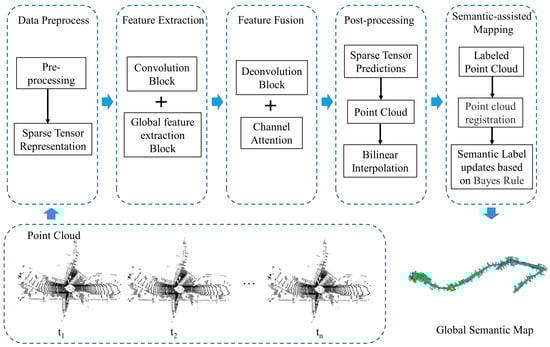
Figure 1.
Architecture of our onboard point cloud semantic segmentation system.
Secondly, we propose a network that uses a transformer module for feature extraction and fusion. In this regard, the feature extraction network learns semantic features of point clouds at different scales by expanding the receptive field of the network through multiple 3 × 3 convolutions, ReLU functions, and down-sampling convolutions with a stride of 2. The feature fusion network combines the results of deconvolution with the corresponding features in the feature extraction layer through concatenation operations. The global feature extraction block (GFEB) and channel attention module (CAM) are designed on this basis. We use the GFEB to learn the importance of different regions of the higher-order semantic features and adjust the corresponding weights to perform feature enhancement. The CAM is used to fuse the different levels of semantic features.
After prediction, the TSR-Net system transforms the sparse tensor-based raster representation into a point cloud and generates a semantic segmentation map of the local scene. After point cloud registration, the TSR-Net system updates semantic labels using Bayes’ rule and eventually obtains a global semantic map.
3.2. Feature Extraction Module
In this module, we expand the perceptual field of the network by multiple 3 × 3 convolutions, ReLU functions, and subsampling convolutions with a stride of 2 to learn the semantic features of point clouds at different scales.
To obtain remote information from the data, we added the transformer encoder module to the deeper layers of the feature extraction network. This module creates an association for each element in the higher-order feature map and distinguishes the importance of features in different regions. It is structured as described below, starting with a given input feature . Positional encoding of the input feature X is achieved by a sparse convolutional operation conv with kernel size equal to stride. Thus, the feature is obtained. The formula is as follows:
The feature is obtained by adding the normalization function after the feature , where :
The attention layer then receives the feature . The attention function computes the query and the dot product of all keys and then divides each dot product by . We combine these queries to form a matrix , . The keys and values are also combined to form a matrix and , . The formula of the attention function is as follows:
where , and are shared parameter matrices, denotes the dimension of query and key, denotes the dimension of value, and the output dimension of the attention function is .
To enhance the computational speed of the self-attentive layer, we use a multi-head attention structure with the number of heads set as 8. Firstly, h different linear mappings of queries, keys, and values are performed. Then the new queries, keys, and values obtained after each mapping are subjected to the parallel operation of the function, respectively, to generate the dimensional output. The formula is as follows:
where the linear transformation parameters are , , and .
is a multi-headed attention layer output. The final output feature is obtained by summing XM with the input feature X through the Layer Norm and ReLU functions, and then recovering the position-encoded deconvolution . The formula is as follows:
3.3. Feature Fusion Module
To enhance the fusion of semantic features at various levels, a channel attention module has been introduced into the feature fusion network. This module creates attention masks in the channel dimension to select critical channels. The input features are compressed to improve computational efficiency. The structure is as follows: firstly, the input features are aggregated using global average and maximum pooling, resulting in and :
The multilayer perceptron (MLP) then accepts these two features, where C is the number of channels and r is the reduction rate. The output features of the MLP are summed element-wise and then passed through a sigmoid function to generate the attentional feature .:
Finally, we obtain the output feature of the module by multiplying and X using the following formula:
3.4. Semantic Map Building
In the process of constructing the semantic map, we transform each frame of the data under the global coordinate system based on LOAM [19] and correlate the before and after frames of the data. Then, the labels of the multi-frame data sequences are updated by Bayes’ rule to generate a global semantic predictive map for the current scene.
We use point-to-edge and point-to-plane mapping calculations to associate the current frame with the previous frame’s point cloud. In the computation, we combine semantic labeling and mapping calculations to weight the labeled similarity and the distance of the corresponding points. First, we denote the edge point as e and the plane point as p. The distances from the point to the edge and plane, respectively, are:
The similarity of labels between corresponding points is calculated as follows:
where is defined as the predicted label distribution for the point . The closest point to is . The association formula is then calculated as follows:
Then, the nonlinear formula is optimized using the Levenberg–Marquardt algorithm. The final result is an optimal inter-frame transformation matrix .
At moment t + 1, we define the label distribution in the semantic map as the conditional probability . According to Bayes’ rule, the point cloud labels in the global map are updated as:
where .
4. Experiment
4.1. Settings
We chose SemanticKITTI as the experimental data for the TSR-Net system. This dataset is semantically labeled with 20 objects, such as fences, motorcyclists, and sidewalks. The dataset consists of 22 sequences scanned by LiDAR in different scenes. Each sequence contains LiDAR point clouds ranging from 200 to 4500 frames. We used sequences 00–10 with semantic annotation for our experiments. A frame was selected from every 5 frames for use in the experiments. The ratio of the experimental data used for training, validation, and testing was 6:2:2.
The evaluation metrics for the TSR-Net system are accuracy (acc) and mIoU. The accuracy is the percentage of all correct predictions made by the system over the total experimental data. The mIoU is an average for each category of the intersection ratio in the dataset. The calculation formula is as follows:
Our system was implemented using the Minkowski Engine on hardware with an Intel Core i9-10980XE (3.0 GHz) and 32 GB RAM memory. The system was parameter optimized using Adam, with a learning rate of 0.0001, momentum of 0.9, batch size of 16, and maximum number of iterations set to 300.
4.2. Semantic Segmentation Results
The feature extraction and fusion module of the TSR-Net system uses 3D-Unet as a baseline model. Figure 2 depicts the system and 3D-Unet’s visualization results on SemanticKITTI.
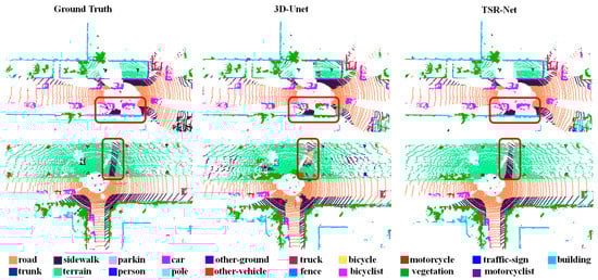
Figure 2.
Visualization of typical segmentation results on the SemanticKITTI dataset. The red boxes highlight the differences in the segmentation results.
As can be seen from the figure, 3D-Unet is able to broadly identify predictive targets. For example, the model can identify pavement information such as cars, roads, and vegetation. However, the segmentation results of 3D-Unet are not accurate enough to delineate effectively the boundaries of large-scale objects. For example, in the first scenario, with multiple cars on the road, the 3D-Unet model was unable to fully recognize the outline information of some of the cars and confused the cars with the vegetation. In addition, the 3D-Unet model also confused buildings at the edge of the road with vegetation and did not fully recognize them. In the second scene, the model was unable to identify accurately the location of the sidewalk in the terrain. In addition, the model is not sufficiently accurate to identify other vehicles and confuses them with cars. Our system is able to effectively address these issues. We have focused our segmentation efforts on the recognition of boundaries of large-scale objects, and the model is also able to identify effectively the contour information of objects such as cars, sidewalks, and parking.
From the above analysis, it is clear that the TSR-Net system improves the real-time semantic segmentation of the system by focusing the segmentation on the boundary recognition of large-scale objects through the global feature extraction and channel attention modules.
In addition, we conducted a comparative analysis of the TSR-Net system and existing models on the large-scale public outdoor dataset SemanticKITTI. Table 1 shows the specific statistical results.

Table 1.
Evaluations of our TSR-Net and existing methods on the SemanticKITTI dataset.
Our system outperformed existing models in the mIoU metric and was 2.2% better than the sub-optimal model based on multiple inputs [20]. Compared with the existing voxelization method [22], which has the best segmentation performance and can be applied in real-time, our results were 2.8% better in the mIoU metric. In terms of segmentation accuracy, our system demonstrated and improvement of 0.6% over the voxelization-based model [21]. Compared to a multi-view-based approach [23], our system performed 7.2% better in terms of mIoU.
The results confirm that the system showed a significant performance improvement in semantic segmentation. Compared with other existing models, our TSR-Net demonstrated a significant advantage in segmenting nine classes of objects such as trucks, roads, parking, and sidewalk.
4.3. Hyperparameters
To test the effectiveness of different modules and the effect of different raster sizes on the system, two comparison experiments were conducted on the SemanticKITTI dataset.
Firstly, to test our proposed GFEB and CAM modules, we added them separately to the 3D-Unet, thus constituting four systems: the baseline model, the baseline model with GFEB added, the baseline model with CAM added, and our TSR-Net. Table 2 shows the comparison results in terms of accuracy, mIoU metrics, and prediction time per frame. Compared to the baseline model, the system showed improvements of 1.6% in the mIoU metric and 16.6 ms in the per-frame prediction time with the addition of GFEB. With the addition of CAM, the system improvements were 3.3% in the mIoU metric and 14.4 ms in the per-frame prediction time. With the addition of both modules, the system improved by 7.6% and 0.9% in the mIoU metric and accuracy, respectively. The prediction time increased by 22.2 ms.
Table 2.
Performance comparison under different model settings.
The results show that both of our proposed modules can enhance the system’s segmentation performance with a small increase in prediction time, and that adding both modules at the same time improves the system most significantly.
Secondly, to test the impact of different raster sizes on the segmentation results, we conducted experiments based on raster sizes of 6, 10, and 20 cm. Table 3 shows the results of our comparison in terms of accuracy, mIoU metrics, and prediction time per frame for different raster sizes.
Table 3.
Segmentation performances of our system using different voxel sizes.
The results show that the larger the raster, the shorter the prediction time for a single frame, and the shortest time for a single frame was 42.1 ms when the raster is 20 cm. However, in terms of the mIoU metric, the smaller the raster the better was the segmentation performance of the system. The best results were obtained at a raster size of 6 cm, with 1.4% higher performance than at 10 cm.
4.4. Efficiency Comparisons
Table 4 represents the results of the efficiency comparison between TSR-Net and the existing model on the GTX 3090 server. Since our system uses sparse convolution for operations, its FLOPs (floating-point operations per second) are calculated as follows:
where Cin and Cout are the numbers of input and output channels, N is the number of effective rasters in the convolutional layer, and K denotes the average convolutional kernel size.
Table 4.
Comparison of the efficiency of our TSR-Net with existing methods.
As can be seen from Table 4, the TSR-Net system has a high number of parameters but only about 65 G of computation, which is more than half the current low [8]. Although we increased the segmentation accuracy by adding global feature extraction and channel attention modules, thus increasing the number of parameters, the value of the FLOPs did not improve significantly. This is due to the fact that our system is based on a sparse tensor. The size of the computation in the system is related to the number of effective rasters in the convolutional layers. The computational effort of the system can be significantly reduced depending on the sparsity of the data.
In addition, we tested the efficiency of the TSR-Net system on the NVIDIA Jetson AGX Xavier platform. We tested the prediction times of the TSR-Net system in eight different power modes for four sequences 00, 02, 04, and 06. Figure 3 shows the statistical average prediction times for the different power modes.
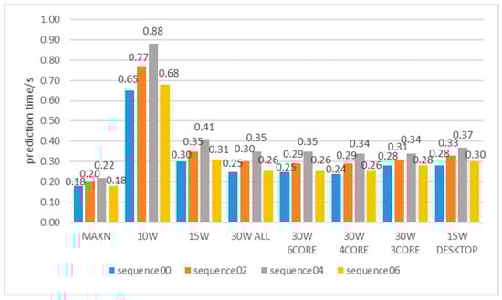
Figure 3.
Inference time of our system on the NVIDIA Jetson AGX Xavier with different device modes.
Our system is able to achieve a prediction speed of 0.19 s per frame in MAXN mode. The system has a prediction speed of 0.75 s per frame in 15 W DESKTOP mode. In addition, the difference in prediction speed is not significant, at about 0.28 s per frame for different CPU cores with 30 W power. As existing LiDAR data is acquired at a frequency of 10 Hz, it takes an average of 0.1 s to acquire one frame of point cloud data. When the time to predict each frame of the point cloud is less than or equal to the acquisition time, it can be concluded that the system can make predictions in real-time. In practice, we sample the point cloud data by sampling one frame of the point cloud sequence for every two frames of data, to achieve a frame rate of 5 FPS. Therefore, it can be considered that a prediction rate of 5 FPS (0.2 s per frame) meets the requirements for real-time applications.
4.5. Semantic Map Building
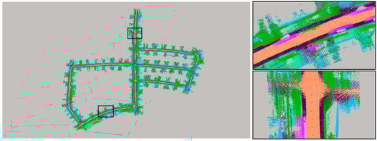
To visualize the real-time segmentation effect of the TSR-Net system, we constructed a global semantic map on the GTX 3090 server. Figure 4 shows the semantic map of our system for the SemanticKITTI dataset 05 sequence scenes. The left-hand side of the image shows a top view of the 05 sequence scene, and the right-hand side shows a zoomed-in view of each of the two partial scenes. During the construction of the semantic map, we censored the data of sequence 05 and updated the semantic labels by taking one frame from every three consecutive frames.
5. Discussion
Our system consists of five parts: data preprocessing, feature extraction, feature fusion, data post-processing, and semantic map construction. The system takes point cloud data as input and outputs a global semantic map. From an efficiency perspective, the data preprocessing and post-processing modules take 5 ms and 1 ms per frame, respectively. The feature extraction and feature fusion modules take 93 ms per frame. The time consumed by the semantic map construction can be neglected. Therefore, our TSR-Net system takes 99 ms per frame for point cloud processing, and outputs semantic segmentation results at a rate of 5 frames per second. The global semantic map module reconstructs the semantic map by taking one frame every two frames of data. Our system uses a grid-based method for processing. Compared with voxel-based models, our system reduces the FLOPs metric by more than half. Compared with fusion models based on multiple data representation forms, our system reduces the FLOPs metric by 174 G.
From a performance perspective, compared with multi-view-based models, our system improved by 7.2% in terms of mIoU indicator. Compared with voxel-based models, our system improved by 6.1% in terms of the mIoU indicator. Compared with fusion models based on multiple data representation forms, our system improved by 2.2% in terms of the mIoU indicator. In addition, our system performs real-time segmentation of point cloud data. Compared with non-real-time models such as RPVNet, our system’s feature extraction and feature fusion modules improved by 2.2% in terms of the mIoU indicator. Compared with real-time models such as (AF)2-S3Net, our system improved by 2.8% in terms of the mIoU indicator.
Finally, from a system perspective, the existing semantic segmentation system Semantic SLAM [24] projects laser point clouds into depth images for semantic segmentation, and then performs point cloud registration and map reconstruction. The focus of the Semantic SLAM system is on pose estimation and semantic map construction. This system utilizes only the RangeNet++ model for semantic segmentation, and our work can replace this. The TSR-Net system focuses on real-time semantic segmentation to solve the problem of real-time system accuracy.
6. Conclusions
We propose a method to solve the problem of onboard semantic segmentation of point clouds for robotic platforms with limited computational resources. The proposed system includes two plug-and-play modules, GFEB and CAM, which are used for learning global contextual information and fusing semantic information at different scales, respectively. After segmenting each single frame, the system uses semantic information to enhance global map building and update labels in the global map with predictions for each frame. To improve the computational efficiency of the system, all net operations are implemented based on a sparse tensor, and pre-processing and post-processing are involved for data transformation between raw 3D points and a sparse tensor.
A series of experiments with SemanticKITTI to test the performance of our system and evaluations against state-of-the-art methods are presented. From the results, we conclude that: (1) the two presented plug-and-play and lightweight modules, GFEB and CAM, can significantly improve the accuracy of semantic segmentation models (+7.6% mIoU) with a limited increase of inference time (16.2 ms per frame). (2) Our system outperforms state-of-the-art methods by 2.2% mIoU and about 18× speedup, resulting in a better balance between accuracy and efficiency for real-time applications. (3) Our system can classify 2.2 million points per second on NVIDIA Jetson AGX Xavier, which demonstrates its ability for use with a variety of robotic platforms with limited computational resources.
Author Contributions
Conceptualization, W.Z.; methodology, F.W.; software, Y.Y.; validation, F.W. and J.Z.; resources, J.Z.; writing—original draft preparation, F.W. and Y.Y.; writing—review and editing, Y.Y. and W.Z.; funding acquisition, F.W. All authors have read and agreed to the published version of the manuscript.
Funding
This research was funded by the National Natural Science Foundation of China, grant number 62103072, Dalian Excellent Youth Talent Fund Project, grant number 2022RY23, and the Fundamental Research Funds for the Central Universities No. 3132023256.
Data Availability Statement
Not applicable.
Conflicts of Interest
The authors declare no conflict of interest.
References
- Teixeira, M.A.S.; Nogueira, R.d.C.M.; Dalmedico, N.; Santos, H.B.; Arruda, L.V.R.d.; Neves, F., Jr.; Pipa, D.R.; Ramos, J.E.; Oliveira, A.S.d. Intelligent 3D Perception System for Semantic Description and Dynamic Interaction. Sensors 2019, 19, 3764. [Google Scholar] [CrossRef]
- Limeira, M.; Piardi, L.; Kalempa, V.C.; Leitao, P.; Oliveira, A.S.d. DepthLiDAR: Active Segmentation of Environment Depth Map Into Mobile Sensors. IEEE Sens. J. 2021, 21, 19047–19057. [Google Scholar] [CrossRef]
- Teixeira, M.A.S.; Neves, F., Jr.; Koubaa, A.; Arruda, L.V.R.d.; Oliveira, A.S.d. DeepSpatial: Intelligent Spatial Sensor to Perception of Things. IEEE Sens. J. 2020, 21, 3966–3976. [Google Scholar] [CrossRef]
- Fang, Y.; Xu, C.; Cui, Z. Spatial transformer point convolution. arXiv 2020, arXiv:2009.01427. [Google Scholar]
- Xu, M.; Ding, R.; Zhao, H. Paconv: Position adaptive convolution with dynamic kernel assembling on point clouds. In Proceedings of the 2021 IEEE/CVF Conference on Computer Vision and Pattern Recognition, Nashville, TX, USA, 19–25 June 2021. [Google Scholar]
- Zhang, Y.; Zhou, Z.; David, P. Polarnet: An improved grid representation for online lidar point clouds semantic segmentation. In Proceedings of the 2020 IEEE/CVF Conference on Computer Vision and Pattern Recognition, Seattle, DC, USA, 14–19 June 2020. [Google Scholar]
- Xu, C.; Wu, B.; Wang, Z. Squeezesegv3: Spatially-adaptive convolution for efficient point-cloud segmentation. In Proceedings of the 2020 European Conference on Computer Vision, Glasgow, UK, 23–28 August 2020. [Google Scholar]
- Tang, H.; Liu, Z.; Zhao, S. Searching efficient 3d architectures with sparse point-voxel convolution. In Proceedings of the 2020 European Conference on Computer Vision, Glasgow, UK, 23–28 August 2020. [Google Scholar]
- Choy, C.; Gwak, J.Y.; Savarese, S. 4d spatio-temporal convnets: Minkowski convolutional neural networks. In Proceedings of the 2019 IEEE/CVF Conference on Computer Vision and Pattern Recognition, Long Beach, CA, USA, 15–21 June 2019. [Google Scholar]
- Zhou, J.C.; Zhang, D.H.; Ren, W.Q. Auto Color Correction of Underwater Images Utilizing Depth Information. IEEE Geosci. Remote. Sens. Lett. 2022, 19, 1–5. [Google Scholar] [CrossRef]
- Chidanand, K.S.; Al-Stouhi, S. Multi-scale voxel class balanced ASPP for LIDAR pointcloud semantic segmentation. In Proceedings of the IEEE/CVF Winter Conference on Applications of Computer Vision, Waikoloa, HI, USA, 5–9 January 2021. [Google Scholar]
- Rosu, R.A.; Schütt, P.; Quenzel, J. Latticenet: Fast point cloud segmentation using permutohedral lattices. arXiv 2019, arXiv:1912.05905. [Google Scholar]
- Zhu, X.; Zhou, H.; Wang, T. Cylindrical and asymmetrical 3d convolution networks for lidar segmentation. In Proceedings of the 2021 IEEE/CVF Conference on Computer Vision and Pattern Recognition, Nashville, TX, USA, 19–25 June 2021. [Google Scholar]
- Zhou, J.C.; Zhang, D.H.; Zhang, W.S. Underwater image enhancement method via multi-feature prior fusion. Appl. Intell. 2022, 52, 16435–16457. [Google Scholar] [CrossRef]
- Strudel, R.; Garcia, R.; Laptev, I.; Schmid, C. Segmenter: Transformer for Semantic Segmentation. In Proceedings of the 2021 IEEE/CVF International Conference on Computer Vision (ICCV), Montreal, QC, Canada, 10–17 October 2021. [Google Scholar]
- Chen, J.; Lu, Y.; Yu, Q. TransUNet: Transformers Make Strong Encoders for Medical Image Segmentation. arXiv 2021, arXiv:2102.04306. [Google Scholar]
- Wei, Y.; Liu, H.; Xie, T.; Ke, Q.; Guo, Y. Spatial-Temporal Transformer for 3D Point Cloud Sequences. In Proceedings of the 2022 IEEE/CVF Winter Conference on Applications of Computer Vision (WACV), Waikoloa, HI, USA, 3–8 January 2022. [Google Scholar]
- Fan, H.; Yang, Y.; Kankanhalli, M. Point 4D Transformer Networks for Spatio-Temporal Modeling in Point Cloud Videos. In Proceedings of the 2021 IEEE/CVF Conference on Computer Vision and Pattern Recognition (CVPR), Nashville, TN, USA, 19–25 June 2021. [Google Scholar]
- Zhang, J.; Singh, S. LOAM: Lidar Odometry and Mapping in Realtime. In Proceedings of the Robotics: Science and Systems 2014, Berkeley, CA, USA, 12–16 July 2014. [Google Scholar]
- Xu, J.; Zhang, R.; Dou, J. Rpvnet: A deep and efficient range-point-voxel fusion network for lidar point cloud segmentation. In Proceedings of the 2021 IEEE International Conference on Computer Vision, Montreal, QC, Canada, 11–18 October 2021. [Google Scholar]
- Zhang, F.; Fang, J.; Wah, B. Deep FusionNet for Point Cloud Semantic Segmentation. In Proceedings of the 2020 European Conference on Computer Vision, Glasgow, UK, 23–28 August 2020. [Google Scholar]
- Cheng, R.; Razani, R.; Taghavi, E. (AF)2-S3Net: Attentive Feature Fusion with Adaptive Feature Selection for Sparse Semantic Segmentation Network. In Proceedings of the 2021 IEEE/CVF Conference on Computer Vision and Pattern Recognition, Nashville, TN, USA, 20–25 June 2021. [Google Scholar]
- Liong, V.E.; Nguyen, T.; Widjaja, S. AMVNet: Assertion-based Multi-View Fusion Network for LiDAR Semantic Segmentation. arXiv 2020, arXiv:2012.04934. [Google Scholar]
- Chen, X.; Milioto, A.; Palazzolo, E.; Giguère, P.; Behley, J.; Stachniss, C. SuMa++: Efficient LiDAR-based Semantic SLAM. In Proceedings of the 2019 IEEE/RSJ International Conference on Intelligent Robots and Systems (IROS), Macau, China, 3–8 November 2019. [Google Scholar]


Disclaimer/Publisher’s Note: The statements, opinions and data contained in all publications are solely those of the individual author(s) and contributor(s) and not of MDPI and/or the editor(s). MDPI and/or the editor(s) disclaim responsibility for any injury to people or property resulting from any ideas, methods, instructions or products referred to in the content. |
© 2023 by the authors. Licensee MDPI, Basel, Switzerland. This article is an open access article distributed under the terms and conditions of the Creative Commons Attribution (CC BY) license (https://creativecommons.org/licenses/by/4.0/).