Replacing Induction Motors without Defined Efficiency Class by IE Class: Example of Energy, Economic, and Environmental Evaluation in 1.5 kW—IE3 Motors

Abstract

This paper shows the results obtained from the study on the variables that have the greatest influence on the decision to replace three-phase induction motors, without a defined efficiency class and installed in industrial applications, with IE3 efficiency class induction motors. The work has been carried out on motors with a nominal power of 1.5 kW due to the availability of laboratory tests that have allowed us to accurately quantify the selected study variables. According to IEC 60034-30, between 0.75 kW and 4 kW is the greatest potential for energy savings in electric motors installed within the industrial sector. The tests carried out have made it possible to assess different operating conditions of the motor: direct power supply from the grid, electronic power supply using scalar control, and electronic power supply using direct torque control. The study has focused on three aspects: energy evaluation, assessing the savings potential; economic evaluation, based on indicators such as Payback Period and Net Present Value; environmental assessment, quantifying the impact indicators proposed by the Methodology for Ecodesign of Energy-related Products (MEErP). A sensitivity analysis has been carried out to quantify, through ratios, different operating points from those directly analyzed in the article.

1. Introduction

Three-phase induction motors still are the most usual electromechanical converters used in industrial applications, mainly in pumps, fans, compressors, manufacturing, and processing of materials, as well as refrigeration equipment [1]. According to IEC 60034-30-1 [2], motors operating the range of 0.75 kW to 375 kW make up most installed units (around 99%). Motors with power from 0.75 kW to 4 kW are identified as the interval with the most significant potential for energy savings (approximately one-third of the total potential). For these reasons, the performance influence of these motors is of great importance in the efficient use of electrical energy, being one more vector to consider in ecodesign and sustainable development policies associated with the consumption of electrical energy [3,4].

In multiple industrial installations, induction motors without a defined efficiency class are still in use because they were selected when the current efficiency classification (IE) was non-existent. The long and useful life of three-phase asynchronous motors and their excellent behavior has meant that their replacement has not been considered.

However, since the establishment of the efficiency classes, manufacturers have improved motor design considerably. Significant efforts focused on increasing motor efficiency, since motors have been seen having a competitive advantage as commercial products [5,6,7].

This paper deals with the dilemma of replacing an installed induction motor, which is working correctly, with another motor with a high-efficiency class and better performance [8].

The decision is not easy and depends on various factors, mainly whether the power is supplied directly from the grid or an electronic converter (in this case, with what type of control) and the operating conditions required of the motor (load index, speed, operating hours, energy price, …).

To answer the above dilemma, objective and quantifiable data are necessary. For this reason, exhaustive laboratory tests are made with several 1.5 kW motors. Obviously, results cannot be directly extrapolated to any other power. However, it could be of great interest to use these results as an initial reference, especially in cases where the machines or the possibility of carrying out the necessary tests are not a priori available.

This paper proposes a study that contemplates energy saving, as well as economic and environmental impact criteria, to aid the decision to replace an IE0 class motor with an IE3 class motor in industrial applications. Since the operating conditions can be very diverse, different operating possibilities as different source types or control techniques were evaluated based on an exhaustive set of laboratory tests. A sensitivity analysis makes it possible to adapt, through the ratios provided, variants that may arise concerning the results directly shown in the article.

The study is organized in the following sections. Section 2 presents the nominal data of the motors and the equipment selected for the study. Section 3 explains the tests carried out and shows the obtained measurements. Section 4 defines the energy, economic, and environmental criteria chosen for the analysis, as well as the hypotheses adopted. Section 5 presents the procedure outputs. In Section 6, a sensitivity analysis was made to quantify different operating points. Section 7 highlights the most relevant aspects of the study and, finally, Section 8 presents the main conclusions derived from the work performed.

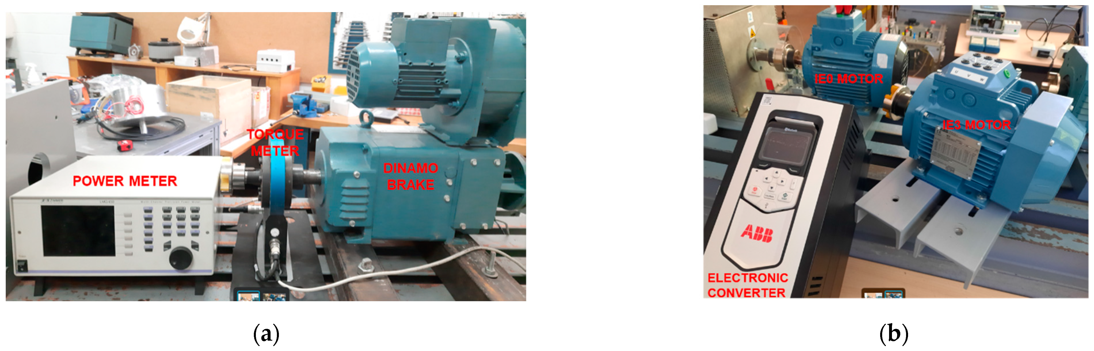
2. Laboratory Setup

The behavior of actual squirrel-cage induction motors was measured in the laboratory. The laboratory setup included the two induction motors subject to analysis, an ac three-phase voltage source, an adjustable speed drive (ASD), as well as measurement equipment.

Regarding the two induction motors used in the experimental setup, the former is manufactured before establishing the efficiency classes and, therefore, it is not classified (labeled IE0). Additionally, the latter is an induction motor with a higher efficiency class (labeled IE3). The nominal parameters of the motors IE0 and IE3 are shown in

Table 1. Nominal values of induction motors.

	Voltage (V)	Current (A)	Speed (rpm)	Power Factor	Weight (kg)
IE0	220	6.6	1420	0.75	16.7
IE3	230	5.6	1439	0.78	22

. Both are three-phase squirrel-cage motors with rated power of 1.5 kW, 50 Hz, and delta connection.

The ASDs used to test the motor under control were the drive ACS 550 (230 V; 7.5 A; 1.5 kW; scalar control), labeled as V/f, as well as the ACS 880 (230 V; 7.5 A; 3 kVA; direct torque control), labeled as DTC.

Finally, the measurements were made by a Zimmer LMG-450 power meter: it was constituted of four channels (600 V and 16 A per channel) [9] and a brake and a torque meter (Kistler 450B100N1B2) (100 Nm; 3350 rpm) [10].

Appendix B shows the laboratory setup used in more detail.

3. Experimental Measurements

To obtain experimental efficiency values, induction motors were tested under variable loads and different power sources. In this case, the power sources were the AC grid, with direct connection and adjustable speed drive with scalar and DTC control. Variable loads are obtained through a hysteresis brake [11,12].

In all the test points determined by different loads, input power, shaft torque, and angular speed were measured.

The presence of harmonics can cause the main difficulty in measurements, using an electronic converter. The electronic converter manufacturer reports that harmonic analysis shows that the systems comply with the IEC 519-2014 [13]. The Total Demand Distortion (TDD) is lower than 5%.

The power meter used incorporates harmonic analysis. It has been verified that the harmonic content is less than 5% in all the measurements. Under these conditions, according to the power meter manufacturer, the accuracy of the input power measurements is not affected.

The input–output method is selected to have a uniform procedure, with power from the grid and the electronic converter. In this way, as the harmonic content introduced by the electronic converter does not exceed 5%, the procedure for efficiency calculation is the same in all cases.

This method does not allow the separation of losses (both the different types of motor losses and the losses of the electronic converter). As the objective of the study proposed in the article is to quantify the global effect of the set of losses, regardless of their type, the authors have not considered it necessary to apply the method 1B (Summation of losses) proposed in the IEC 60034-2-1 [14].

If it is required to obtain the separation of losses in the motor and the losses of the electronic converter, and the IEC 60034-2-3 [15] must be applied. Various studies analyze this procedure in depth [16,17,18].

3.1. Direct Power Supply from the ac Grid

In this test, induction motors were connected to the AC grid (230 V/50 Hz) (laboratory AC grid) and tested, as mentioned above. From the experimental data, efficiency was calculated and presented in Figure 1. Note that efficiency was calculated according to standard 60034-2-1 (input–output method). The load index was defined as the ratio between the output and the nominal power (P/P_n).

3.2. Scalar Control (V/f)

Another set of measurements was made with an adjustable speed drive with scalar control, setting the V/f value. In these cases, the input power was measured at the input of the ASD. The measurements were organized as follows:

• Five-speed references are defined as a % in relation to the motor-rated synchronous speed (20%, 40%, 60%, 80%, and 100%).
• The load index has been defined as the ratio between the torque and the nominal torque (M/Mn).

Figure 2 presents the calculated efficiency, where solid lines correspond to the IE3 motor, and dashed lines correspond to the IE0 motor.

3.3. Direct Torque Control (DTC)

Finally, another set of measurements was obtained with the ASD under open-loop DTC control. The measurements were organized as follows:

• Five-speed references are defined as a % in relation to the motor-rated synchronous speed (20%, 40%, 60%, 80%, and 100%).
• The load index has been defined as the ratio between the torque and the nominal torque (M/Mn).

Figure 3 presents the calculated efficiency, where solid lines correspond to the IE3 motor, and dashed lines correspond to the IE0 motor.

4. Energy Saving, Economic and Environmental Criteria

In this section, mathematical modeling for energy saving, as well as economic and environmental criteria, are presented.

4.1. Energy Saving

Equation (1) shows the procedure to calculate the annual energy savings that can be obtained by replacing the IE0 motor with the IE3 motor:

$$\mathrm{ES}={\displaystyle \sum }_{\mathrm{workcycles}}{P}_n\cdot h\cdot \mathrm{LI}\cdot \left(\frac{1}{{\eta }_{\mathrm{IE}0}}-\frac{1}{{\eta }_{\mathrm{IE}3}}\right)$$

(1)

where:

-

ES = annual energy savings (kWh/year).

-

Pn = rated power of the motor (kW).

-

h = operating time per year (hours/year).

-

LI = load index.

-

η_IE0 = IE0 motor efficiency, at load index established.

-

η_IE3 = IE3 motor efficiency, at load index established.

In many applications, the load index is not constant, so motors run out of their rated conditions. Therefore, the work cycles that can be found are very different and varied. For this reason, the calculation was made by setting a fixed load index and modifying the number of operating hours. In this way, energy saving can be calculated for each work cycle as a sum of the different operating conditions each cycle contains [19].

The option to apply typical fixed and variable speed general-purpose drive duty cycles, as has been conducted in many previous studies [20,21], is also very interesting. Still, we have decided to leave it open since the existing possibilities at the level of industrial applications are very diverse.

4.2. Economic Criteria

To calculate the annual economic savings, the cost of electrical energy [22] has been applied directly to the result of Equation (1):

$$\mathrm{ECS}=\mathrm{ES}\cdot c$$

(2)

where:

-

ECS = Annual economic savings (€/year).

-

c = electricity cost (€/kWh).

To assess whether the necessary economic investment is profitable [23,24], the Payback Period (PP) and the Net Present Value (NPV) have been used, considering an annual increase in the cost of electrical energy to calculate the NPV of 2%:

$$\mathrm{PP}\left(\mathrm{years}\right)=\frac{I}{\mathrm{ECS}}$$

(3)

$$\mathrm{NPV}(€)={{\displaystyle \sum }}_{\mathrm{T}=0}^T\left(\frac{\mathrm{ECS}}{{(1+\mathrm{i})}^T}\right)-I$$

(4)

where:

-

I = investment (€ EUR).

-

i = rate of return.

-

T = number of time periods.

4.3. Environmental Criteria

Assessment of improvements in environmental impact derived from the energy savings was made using the Methodology for Ecodesign of Energy-related Products (MEErP). This methodology is based on the regulation formulated by the European Union (EU) through the use of a spreadsheet that performs a Life Cycle Assessment (LCA) in a simplified way [25]. Although the MEErP allows one to assess the environmental impact throughout the life cycle (from production, to use, transportation, and final recycling) by means of different impact ratios, in this study, for quantity comparison, only the phase usage is considered because it is where energy savings have an influence [26,27]. The indicators selected for the study are listed below:

-

Total Energy (GER)

-

Water (process)

-

Waste, non-hazardous/landfill

-

Greenhouse gases in GWP100

-

Acidification, emissions

-

Heavy metals

-

Particulate matter (PM, dust)

-

Eutrophication

In this analysis, a relative value of the reduction in environmental impact was considered more important than the absolute amounts achieved in each indicator. For this reason, in the results shown below, the Relative Environmental Indicator (REI) has been calculated for each indicator based on:

$$\mathrm{REI}\left(i\right)=\frac{\mathrm{TEI}\left(i\right)\mathrm{IE}3}{\mathrm{TEI}\left(i\right)\mathrm{IE}0}$$

(5)

where:

-

TEI (i) IE3 = Total Environmental Impact (for the indicator i) using the IE3 motor.

-

TEI (i) IE0 = Total Environmental Impact (for the indicator i) using the IE0 motor.

Additionally, based on the REI for each selected indicator, the Environmental Impact Global Ratio (EIGR) was calculated as:

$$\mathrm{EIGR}=\frac{{{\displaystyle \sum }}_{\mathrm{i}=1}^n\mathrm{REI}\left(i\right)}{n}$$

(6)

5. Methodology Outputs

In this section, results obtained by application of the methodology presented above are presented.

5.1. Energy Saving Results

Figure 4, Figure 5 and Figure 6 present the energy savings calculated using Equation (1) under different operating conditions. Figure 4 corresponds to the analysis with the motors connected directly to the AC grid. Figure 5 and Figure 6 present the analysis of the motors with scalar control and DTC, respectively.

In all tests, three different load indexes (LI) were selected, 1 or full load, 0.75 (3/4 load), and 0.5 or half load. Furthermore, in the case of feeding through ASD (Figure 5 and Figure 6), the performance at synchronous and half-synchronous speeds is presented.

From these figures, it could be highlighted that:

• According to Figure 4, it can be seen how the energy savings grow proportional to the load index if motors are directly fed from the grid.
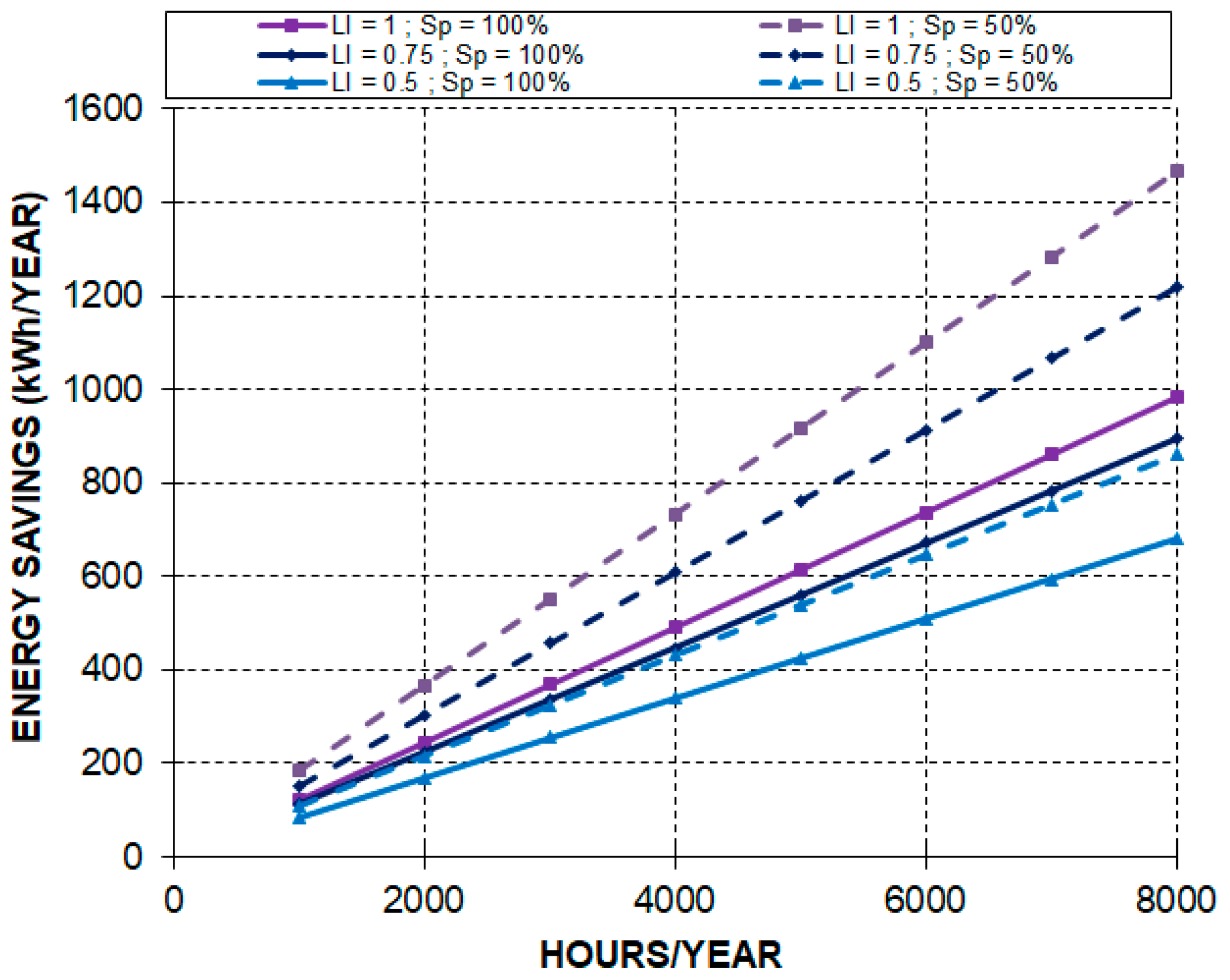
• In the case of V/f control, Figure 5 shows the energy savings are greater at high speeds if the load index is greater than 0.75. However, for low index loads (below 0.5), greater energy saving is obtained with the lowest speeds.
• Finally, in Figure 6, with DTC, energy savings are greater at low speeds with independence of load index.

5.2. Economic Results

In this section, the economic results are computed from the same operating conditions defined in Section 5.1 and using Equations (2)–(4).

The economic data used as a basis are [28,29]:

• An electricity cost of 0.242 € EUR/kWh. This value corresponds to the average cost among the 27 countries of the European Union during the first half of 2022. An annual increase in this cost of 2% has been considered.
• Investment in the purchase of the IE3 motor: 480 € EUR.
• Investment in the purchase of the ACS 550 electronic converter with scalar control: 770 € EUR.
• Investment in the purchase of the electronic converter with direct torque control ACS 880: 1400 € EUR.
• Rate of return: 3%.
• Number of time periods: 12.

Note that, as the objective of this study is the complete replacement of the installed equipment, the total cost of the equipment has been considered as an investment. Therefore, in the cases of the IE3 motor with electronic control, the cost of the motor and the electronic converter has been added.

Figure 7, Figure 8 and Figure 9 present the Payback Period and the Net Present Value analysis. Figure 7 corresponds to the analysis with the motors connected directly to the AC grid. Figure 8 and Figure 9 present the analysis of the motors with scalar control and DTC, respectively.

From these figures, it could be highlighted that:

• In the case of direct connection to the grid (Figure 7), the Payback Period is roughly half of the number of time periods established (six years) for full-load performance and 2000 h/year, 0.75 load and 3000 h/year, and half-load and 4000 h/year. The NPV is positive at 1000 h/year at full load, 1500 h/year at 0.75 load, and 2000 h/year and half load.
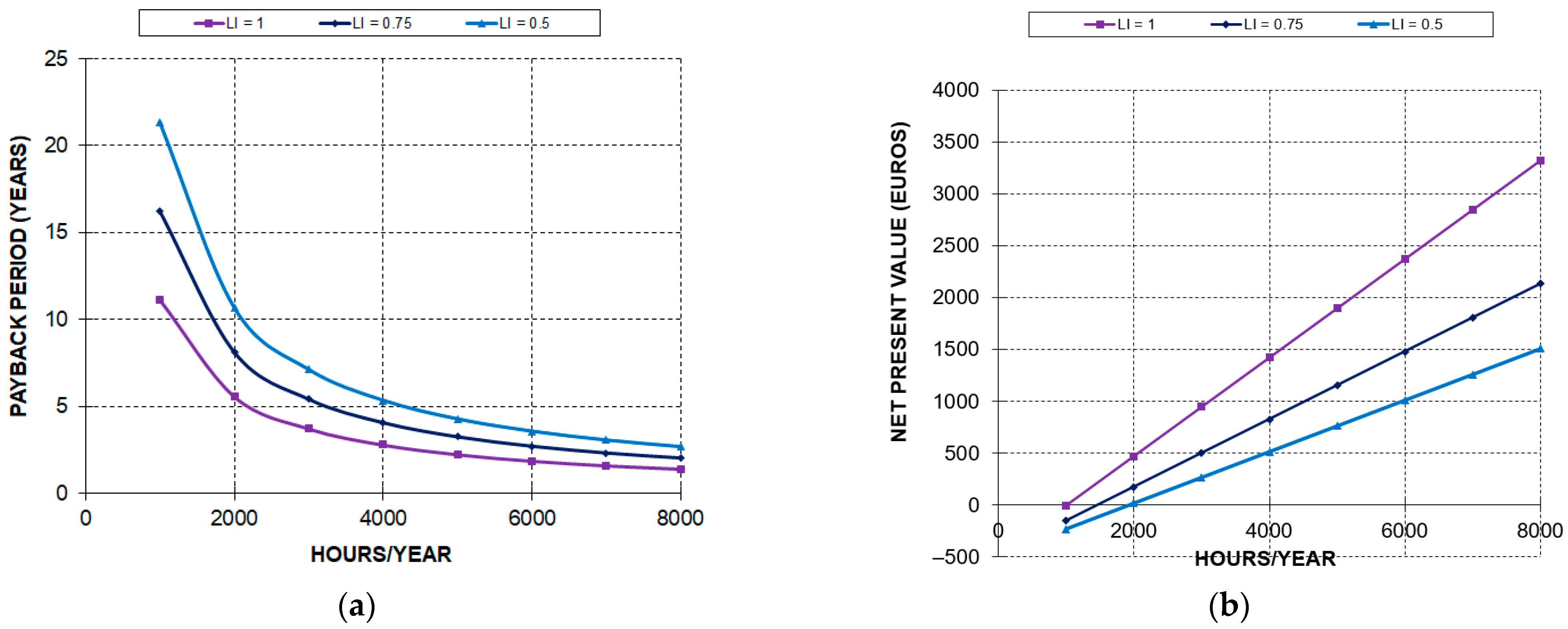
• With scalar control (Figure 8), the Payback Period is roughly half of the number of time periods established (six years) for the two analyzed speeds. The motor has a 0.75 load at rated speed for 5000 h/year. For load index below 0.75 and half speed, it is not possible to go below the six-year period. The NPV is positive at 1000 h/year at full load, 1500 h/year at 0.75 load, and 2000 h/year and half load. The NPV is positive from 2000 h/year at full load and rated speed or 2500 h/year at half speed, even more for a 0.75 load index at half-rated speed. In contrast, the value of hours/year must grow to 4500 or even to 6000 for half-load and half-rated speed.
• When the DTC is applied the Payback Period, it is not below the established period in any of the analyzed cases. The NPV take positive values from 4000 h/year to 6500 h/year in case of full-load and half-rated speed and 0.75 load index and rated speed, respectively. It must be noted that, for half-load and rated speed, the NPV is always negative in all the hours/year range.

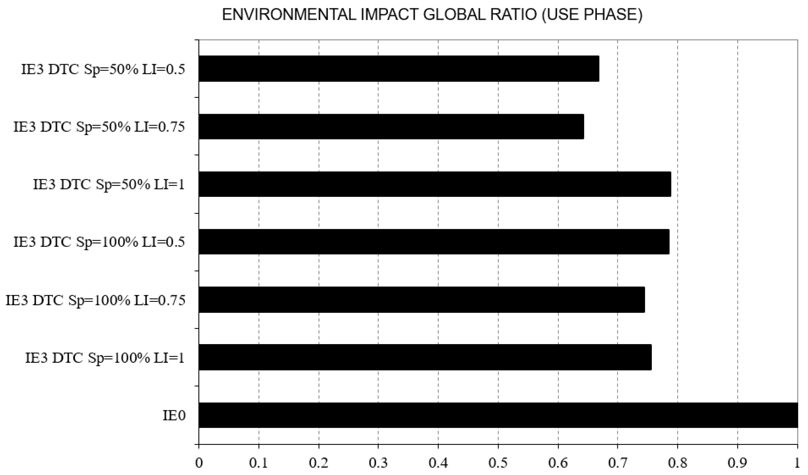
5.3. Environmental Impact Results

In this section, the environmental impact is calculated from Equations (5) and (6) considering the same operating conditions as the other tests. The Environmental Impact Global Ratio (EIGR) for the use phase is calculated as a difference in values with respect to the operation of the IE0 motor, and results are plotted in Figure 10, Figure 11 and Figure 12. Figure 10 corresponds to the analysis with the motors connected directly to the AC grid. Figure 11 and Figure 12 present the analysis of the motors with scalar control and DTC, respectively.

From these figures, it can be established that the environmental impact is always lower than case base if the motor is connected directly to the grid (Figure 10). Moreover, with the scalar control (Figure 11), the impact is reduced between, 20% to 35% in all cases, and, finally, with the DTC (Figure 12), the impact reduction climbs to 35% for low speeds and non-full loads.

6. Sensitivity Analysis

A sensitivity study of the most influential variables was conducted to obtain more information before the replacement decision [30,31]. In all the cases, the variables to analyze the sensitivity are the running hours, considered in the range between 1000 and 8000 h/year, as well as the energy difference for different values between 2 and 12 percent.

In all cases, the reference operating point was set to annual operating hours at 4000 h/year and a 0.08 pu difference in performance between motors (reference value = 1).

The results of the sensitivity analysis shown in this section are presented using colored graphs to easily observe the variation trends. The exact relative values at each point in the matrix are given in Appendix A (reference value = 1 = white color).

6.1. Energy Saving Analysis

Looking at Equation (1), it is clear that the variables that most significantly impact energy savings are the annual operation number of hours and the efficiency difference between motors. This fact is also visible in Figure 13, where the strong red color is found for the high values of motor running and also when there is the biggest efficiency difference between motors.

6.2. Economic Analysis

The economic analysis was made from Equations (2)–(4).

Firstly, the Payback Period was analyzed, and it can be seen in Figure 14. The Payback Period was extremely influenced by the initial investment, the operating time per year, and the electricity cost.

Secondly, the Net Present Value (NPV) is influenced by the energy cost, the initial investment required, and the rate of return. For this reason, to reflect the influence of the three variables separately, Figure 15, Figure 16 and Figure 17 are showed. Figure 15 presents the NPV sensitivity analysis for variations in the cost of energy, with increases of 25% and 50%. Figure 16 shows the analysis results for variations in the initial investment of 50% and 100%. Finally, Figure 17 includes the analysis when variations in the rate of return are set to 50% and 100%. In all cases, the economic reference values adopted are electricity cost equal to 0.242 €/kWh, a 480 € EUR initial investment, and a 3% of rate of return.

In Figure 15, Figure 16 and Figure 17, part (a) represents the trend, corresponding to the base case adopted as reference. Parts (b) and (c) of these Figures represent the NPV variation trend with respect to the value adopted as a base in part (a), in order to have a visual trend of how they affect the variations in the cost of electricity, in the investment made, and the rate of return, respectively. This was performed with respect to the base values (the exact numerical quantities can be found, in all cases, in the tables shown in Appendix A).

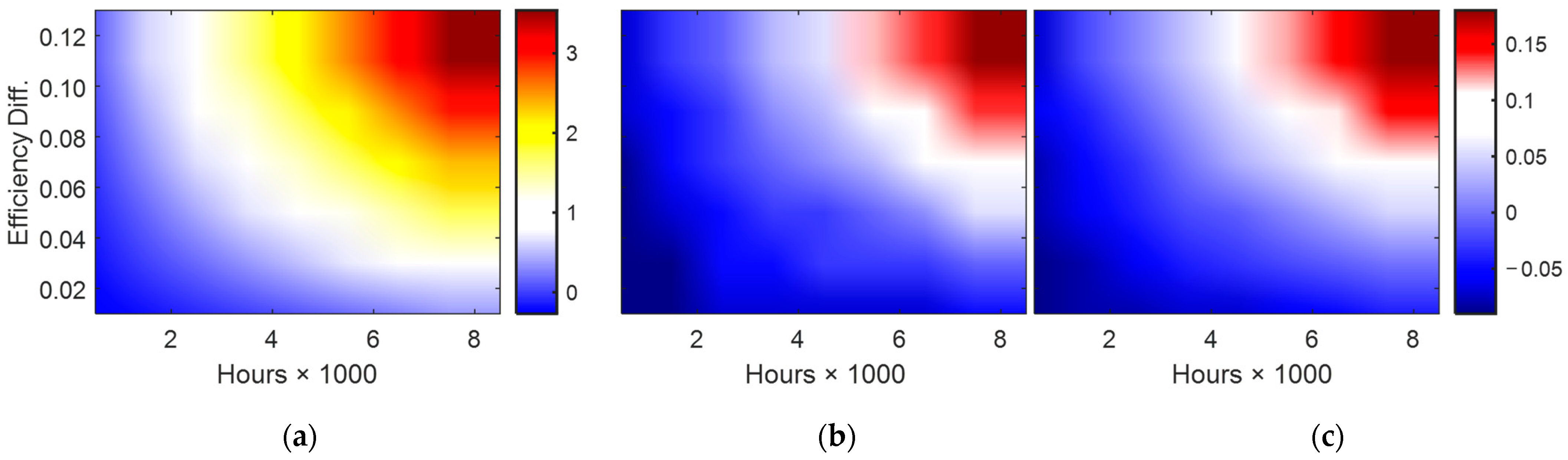
6.3. Environmental Analysis

The sensitivity analysis was carried out using Equations (5) and (6). In this case, as the adopted indicator already shows a relative value (EIGR, Environmental Impact Global Ratio) between the same operating points for the two motors, there is no base reference value.

The different EIGRs obtained are shown in

Table 2. Sensitivity analysis: Environmental Impact Global Ratio (EIGR) values.

Efficiency Difference	EIGR
0.02	0.65
0.04	0.64
0.06	0.62
0.08	0.61
0.1	0.59
0.12	0.58

Note: Use phase, load index = 1.

. As the calculated ratios do not change with the number of annual operating hours, they are shown based exclusively on the two motors performance difference. The corresponding values for the use phase and for full load operation are displayed (load index = 1).

7. Discussion

Based on the results obtained, the most important aspects to consider are related to energy saving, economic aspects, and environmental impact, which are highlighted below.

Regarding energy savings, obviously, any of the proposed substitutions, regardless of the point of operation, generate savings. Performance with the motor directly connected to the grid and high load index obtains the greatest savings potential. Similarly, if the scalar electronic control is considered, greater savings are obtained at the highest speeds, except for operations with a load index equal to or less than 0.5 and speed equal to or less than 50% of the nominal synchronous speed. To the contrary, with direct torque control, it is remarkable that the greatest savings potential is achieved for the lowest speeds.

The approach that the authors have wanted to give to the proposed article impacts the use of commercial equipment that incorporates scalar control and direct torque control techniques. The in-depth study and analysis of the optimization of these control techniques [32,33,34] goes beyond the objective proposed in the article, which is essentially intended to be an aid in deciding whether or not it is convenient to make the economic investment in the acquisition of more efficient motors or industrial speed regulation equipment already available on the market.

In the economic analysis, a criterion for a good investment—a Payback Period equal to or less than half of the estimated operating life, and with a positive Net Present Value, was established. In the direct feeding of the grid, the criterion is accomplished from 2000 h per year with full load operation, from 3000 h per year with a load index of 0.75, and, at half load, we approach 4000 h per year of operation. In the case of scalar control, the conditions are met after 4000 annual hours of operation at full load always and at load index 0.75 for high speeds. However, the running annual hours must be greater than 8000 to be economically profitable if the operation is at half or ¾ full load and speeds around 50% of the nominal synchronous speed. In the case of direct torque control, no analyzed operating point meets the pre-established profitability criteria. The margin of the Payback Period must be extended to a value close to the initial estimated life and operation after 7000 h/year to be consistent with the criterion of profitability if the load index is greater than 0.5. Worst cases are for lower index loads, where the hours of operation should be extended to 8000 per year.

From the point of view of environmental impact, all the investments and operating points analyzed are favorable. The most significant impact reductions are achieved for the operation of the motor connected to the grid, at any load index. With scalar electronic control, the best impact rates are achieved for the higher speeds, while direct torque control achieves high impact improvements for the lower speeds.

The sensitivity analysis allows easy adaptation and calculations to make different scenarios for a given application with a variable operating point. As an example, from this analysis and from the coefficients determined, profitability maps can be obtained according to the criteria adopted, such as the one shown in Figure 18. This Figure was made with the case studied in the article, establishing as profitability criteria and obtaining a Payback Period less than half of the estimated life time (PP < T/2) and a positive Net Present Value (NPV > 0).

8. Conclusions

Replacing appliances, devices, or equipment that still work correctly with others that present technological improvements is a choice that can lead to some advantages. Despite that, the decision should be based on objective data and rigorous analysis.

In this article, the element to be replaced is an induction motor of the unclassified efficiency category with another induction motor with an efficiency class established according to the standard IEC 60034-30-1.

The decision is not unique and direct, since the operating conditions of the motor in an industrial application can be very diverse. Various modes of operation were proposed, with the motor fed directly from the industrial grid or using an electronic converter with different types of control. It was also necessary to analyze different load index and different speeds in the case of the electronic control.

To help decision-making, criteria for energy saving, economic profitability, and environmental impact were defined. From the point of view of energy saving and environmental impact, practically all the operating conditions analyzed show favorable results for replacement.

From the economic aspect, the greatest variability of results appears. It is necessary to establish the criterion of economic profitability clearly. In the presented study, the criterion regarded two economic indicators: the Payback Period and the Net Present Value. Based on the results obtained and in a simplified way, for a load index equal to or greater than 0.75, it can be concluded that, when the motor works directly from the grid after 2000 h per year, or with scalar electronic control after 4000 h of annual operation, the results are favorable. In operation with direct torque control, the necessary economic investment in the electronic equipment reduces the economic profitability to several annual operating hours greater than 7000.

The ratios calculated in the sensitivity analysis make it possible to correct, in a relatively simple and direct way, possible changing scenarios that the multiple operating possibilities may offer.

References

- De Almeida, A.T.; Falkner, H.; Fong, J.; Jugdoyal, K. EuP Lot 30: Electric Motors and Drives; Final Report; University of Coimbra: Coimbra, Portugal, 2014. [Google Scholar]
- IEC 60034-30-1; Standard on Efficiency Classes for Low Voltage AC Motors. 2014. Available online: https://webstore.iec.ch/publication/136 (accessed on 11 April 2023).
- Ecodesign Electric Motors. Commission Regulation (EU) No 4/2014 of 6 January 2014 Amending Regulation (EC) No 640/2009 Implementing Directive 2005/32/EC of the European Parliament and of the Council with Regard to Ecodesign Requirements for Electric Motors. Available online: https://www.eumonitor.eu/9353000/1/j9vvik7m1c3gyxp/vjgp6pule7zm (accessed on 11 April 2023).
- De Almeida, A.T.; Ferreira, F.J.T.E.; Fong, J. Perspectives on Electric Motor Market Transformation for a Net Zero Carbon Economy. Energies 2023, 16, 1248. [Google Scholar] [CrossRef]
- Bortoni, E.C.; Bernardes, J.V.; da Silva, P.V.; Faria, V.A.; Vieira, P.A. Evaluation of manufacturers strategies to obtain high-efficient induction motors. Sustain. Energy Technol. Assess. 2019, 31, 221–227. [Google Scholar] [CrossRef]
- Aishwarya, M.; Brisilla, R.M. Design of Energy-Efficient Induction motor using ANSYS software. Results Eng. 2022, 16, 100616. [Google Scholar] [CrossRef]
- Lu, S.-M. A review of high-efficiency motors: Specification, policy, and technology. Renew. Sustain. Energy Rev. 2016, 59, 1–12. [Google Scholar] [CrossRef]
- Goman, V.; Prakht, V.; Kazakbaev, V.; Dmitrievskii, V. Comparative Study of Induction Motors of IE2, IE3 and IE4 Efficiency Classes in Pump Applications Taking into Account CO2 Emission Intensity. Appl. Sci. 2020, 10, 8536. [Google Scholar] [CrossRef]
- Available online: https://www.zes.com/en/Products/Precision-Power-Analyzers/LMG450 (accessed on 11 April 2023).
- Available online: https://www.kistler.com/ES/en/cp/torque-measuring-flange-system-kitorq-rotor-measuring-ranges-100-to-10000-nm-4550a/P0000244 (accessed on 11 April 2023).
- Tabora, J.M.; Tostes, M.E.D.L.; Bezerra, U.H.; De Matos, E.O.; Filho, C.L.P.; Soares, T.M.; Rodrigues, C.E.M. Assessing Energy Efficiency and Power Quality Impacts Due to High-Efficiency Motors Operating Under Nonideal Energy Supply. IEEE Access 2021, 9, 121871–121882. [Google Scholar] [CrossRef]
- Martinez, M.A.; Gutierrez, J.M.; Malagon, S.M.; Mendoza, F.; Rodriguez, J. A speed performance comparative of field oriented control and scalar control for induction motors. In Proceedings of the 2016 IEEE Conference on Mechatronics, Adaptive and Intelligent Systems (MAIS), Hermosillo, Mexico, 20–22 October 2016. [Google Scholar] [CrossRef]
- IEC 519; Recommended Practice and Requirements for Harmonic Control in Electric Power Systems. 2014. Available online: https://edisciplinas.usp.br/pluginfile.php/1589263/mod_resource/content/1/IEE%20Std%20519-2014.pdf (accessed on 11 April 2023).
- IEC 60034-2-1; Standard Methods for Determining Losses and Efficiency from Tests (Excluding Machines for Traction Vehicles). 2014. Available online: https://webstore.iec.ch/publication/121 (accessed on 11 April 2023).
- IEC 60034-2-3; Rotating Electrical Machines—Part 2–3: Specific Test Methods for Determining Losses and Efficiency of Converter-Fed AC Motors. 2020. Available online: https://webstore.iec.ch/publication/30919 (accessed on 11 April 2023).
- Boglietti, A.; Cavagnino, A.; Cossale, M.; Tenconi, A.; Vaschetto, S. Efficiency Determination of Converter-Fed Induction Motors: Waiting for the IEC 60034-2-3 Standard. In Proceedings of the 2013 IEEE Energy Conversion Congress and Exposition, Denver, CO, USA, 15–19 September 2013. [Google Scholar] [CrossRef]
- Aminu, M.; Mushenya, J.; Barendse, P.S.; Khan, M.A. Converter-fed Induction Motor Efficiency Measurement under Variable Frequency/Load Points: An Extension of the IEC/TS 60034-2-3. In Proceedings of the 2019 IEEE Energy Conversion Congress and Exposition (ECCE), Baltimore, MD, USA, 29 September 2019–3 October 2019. [Google Scholar] [CrossRef]
- Karkkainen, H.; Aarniovuori, L.; Niemela, M.; Pyrhonen, J. Converter-Fed Induction Motor Efficiency: Practical Applicability of IEC Methods. IEEE Ind. Electron. Mag. 2017, 11, 45–57. [Google Scholar] [CrossRef]
- Rachev, S.; Dimitrov, L.; Ivanov, I.; Karakoulidis, K. Study the Effects of No Nominal Conditions on the Performance of High Efficiency Induction Motor. In Proceedings of the 2017 IEEE International Conference on Energy and Environment (CIEM 2017), Bucharest, Romania, 19–20 October 2017. [Google Scholar] [CrossRef]
- IEC 61800-9-2; Adjustable Speed Electrical Power Drive Systems—Part 9-2: Ecodesign for Power Drive Systems, Motor Starters, Power Electronics and Their Driven Applications—Energy Efficiency Indicators for Power Drive Systems and Motor Starters. 2017. Available online: https://webstore.iec.ch/publication/31527 (accessed on 11 April 2023).
- Aarniovuori, L.; Karkkainen, H.; Anuchin, A.; Pyrhonen, J.J.; Lindh, P.; Cao, W. Voltage-Source Converter Energy Efficiency Classification in Accordance With IEC 61800-9-2. IEEE Trans. Ind. Electron. 2020, 67, 8242–8251. [Google Scholar] [CrossRef]
- Saidur, R. A review on electrical motors energy use and energy savings. Renew. Sustain. Energy Rev. 2010, 14, 877–898. [Google Scholar] [CrossRef]
- Jardot, D.; Eichhammer, W.; Fleiter, T. Effects of economies of scale and experience on the costs of energy-efficient technologies—Case study of electric motors in Germany. Energy Effic. 2010, 3, 331–346. [Google Scholar] [CrossRef]
- Gugaliya, A.; Naikan, V. A model for financial viability of implementation of condition based maintenance for induction motors. J. Qual. Maint. Eng. 2020, 26, 213–230. [Google Scholar] [CrossRef]
- Methodology for Ecodesign of Energy-Related Products, MEErP, Final Report. 2011. Available online: https://op.europa.eu/s/yGHF (accessed on 11 April 2023).
- Torrent, M.; Martínez, E.; Andrada, P. Life cycle analysis on the design of induction motors. Int. J. Life Cycle Assess. 2011, 17, 1–8. [Google Scholar] [CrossRef]
- Torrent, M.; Martinez, E.; Andrada, P. Assessing the environmental impact of induction motors using manufacturer’s data and life cycle analysis. IET Electr. Power Appl. 2012, 6, 473–483. [Google Scholar] [CrossRef]
- Available online: https://new.abb.com/motors-generators/iec-low-voltage-motors/general-performance-motors (accessed on 11 April 2023).
- Available online: https://new.abb.com/drives/low-voltage-ac/industrial-drives (accessed on 11 April 2023).
- Rai, K.; Seksena, S.B.L.; Thakur, A.N. Economic Efficiency Measure of Induction Motors for Industrial Applications. Int. J. Electr. Comput. Eng. IJECE 2017, 7, 1661–1670. [Google Scholar] [CrossRef]
- Rajinder; Sreejeth, M.; Singh, M. Sensitivity Analysis of Induction Motor Performance Variables. In Proceedings of the 2016 IEEE 1st International Conference on Power Electronics, Intelligent Control and Energy Systems (ICPEICES), Delhi, India, 4–6 July 2016. [Google Scholar] [CrossRef]
- Paes, R.; Toner, B.; Bankay, G.; Agashe, G. Energy Optimization for Adjustable-Speed Drive Applications: Increasing Efficiency to Cut Costs and Preserve Assets. IEEE Ind. Appl. Mag. 2021, 27, 37–46. [Google Scholar] [CrossRef]
- Lee, K.; Qi, J. Energy Efficiency Performance Evaluation of Direct Torque and Flux Control in Induction Machines Driven by Adjustable Speed Drives. In Proceedings of the 2020 IEEE Energy Conversion Congress and Exposition (ECCE), Detroit, MI, USA, 11–15 October 2020. [Google Scholar] [CrossRef]
- Zhang, Z.; Bazzi, A.M. Robust Sensorless Scalar Control of Induction Motor Drives with Torque Capability Enhancement at Low Speeds. In Proceedings of the 2019 IEEE International Electric Machines & Drives Conference (IEMDC), San Diego, CA, USA, 12–15 May 2019. [Google Scholar] [CrossRef]