Deep PCA-Based Incipient Fault Diagnosis and Diagnosability Analysis of High-Speed Railway Traction System via FNR Enhancement

Abstract

In recent years, the data-driven based FDD (Fault Detection and Diagnosis) of high-speed train electric traction systems has made rapid progress, as the safe operation of traction system is closely related to the reliability and stability of high-speed trains. The internal complexity and external complexity of the environment mean that fault diagnosis of high-speed train traction system faces great challenges. In this paper, a wavelet transform-based FNR (Fault to Noise Ratio) enhancement is realised to highlight incipient fault information and a Deep PCA (Principal Component Analysis)-based diagnosability analysis framework is proposed. First, a scheme for FNR enhancement-based fault data preprocessing with selection of the intelligent decomposition levels and optimal noise threshold is proposed. Second, fault information enhancement technology based on continuous wavelet transform is proposed from the perspective of energy. Further, a Deep-PCA based incipient fault detectability and isolatability analysis are provided via geometric descriptions. Finally, experiments on the TDCS-FIB (Traction Drive Control System–Fault Injection Benchmark) platform fully demonstrate the effectiveness of the method proposed in this paper.

1. Introduction

Research on high-speed train FDD (Fault Detection and Diagnosis) along with safety warnings to eliminate or reduce safety accidents is key to the sustainable and healthy development of the high-speed rail system, and has become an urgent need for continued high-speed rail development all over the world. The electric traction system is the core part of CRH (China Railway High-speed) trains; as shown in Figure 1, it consists of a pantograph, traction transformer, impulse rectifier, traction inverter, and induction motor. Due to the complex and changing environment of train operation, the traction systems on board experience many harsh environments, which can lead to a variety of incipient faults. Meanwhile, environmental noise presents enormous challenges for incipient FDD in high-speed train traction systems, and has attracted more and more attentions recently [1,2,3,4].

Generally, the running data collected from high-speed trains involves a lot of noise. Among the traditional noise reduction methods, wavelet transform-based noise reduction has been widely used due to its high reliability and easy realization. The main factors affecting wavelet denoising are wavelet decomposition coefficient and threshold selection, which have motivated work in recent years. Adaptive wavelet denoising methods [5,6,7,8] involving adjacent coefficients and adaptive threshold design can take into consideration local features and noise at different decomposition levels. Further, multi-wavelet denoising methods [9,10,11,12,13] can be realized by merging adjacent coefficients to achieve a unified multi-wavelet threshold. Wavelet image thresholding schemes have been proposed in [14,15,16,17,18] by combining TI (translation-invariant) adjacent coefficients with non-TI adjacent coefficients. Adaptive wavelet threshold denoising methods based on SURE estimation (Stein Unbiased Risk Estimation) were investigated in [19,20,21,22] for selection of optimal thresholds and window sizes, which were subsequently extended to the redundant DT-CWT (dual-tree complex wavelet transform). The thresholds were divided into global thresholds and local thresholds, based on which soft threshold concept-based optimal threshold selection methods were proposed [23,24,25,26,27] by analysing the values of SNR (signal-to-noise ratio), MSE (mean square error), and RMSE (root mean square error). Noise estimation is required in traditional threshold design, which limits the threshold accuracy and its applications. To solve this problem, HBTEs (histogram-based threshold estimations) with different noise levels were provided in [28,29,30,31,32]. Similarly, PSR (Peak-Sum Ratio)-based noise reduction schemes have been proposed in [33,34,35], allowing the limitations on noise estimation to be removed.

In recent decades, as the representative of multivariate statistical analysis, PCA (Principal Component Analysis)-based incipient FDD schemes have been widely used, including in applications on high-speed train traction systems. KPCA (Kernel Principal Component Analysis) for removal of the non-Gaussian and nonlinearity of data was proposed in [36] by projecting the data to higher dimensions through a kernel function. Based on this, and in combination with SVM (Support Vector Machine) [37], incipient fault information can be further investigated. The concept of Deep-PCA, combining PCA theory with deep learning, as in [38], can further improve incipient fault detection capability. However, little research has been conducted on PCA-based diagnosability analysis, and research on detectability and isolatability analysis under the Deep-PCA framework is especially lacking.

In this paper, the wavelet transform-based FNR (Failure to Noise Ratio) enhancement is realised to highlight incipient fault information and diagnosability analysis under a Deep-PCA framework. The main contributions are as follows:

(1)

An intelligent decomposition levels selection scheme is proposed by quantifying the similarity of detail components, and the selection of noise threshold is determined and optimized to further improve the accuracy of noise reduction.

(2)

A continuous wavelet transform-based fault information enhancement approach is proposed from the perspective of fault energy.

(3)

A Deep-PCA based diagnosability analysis is provided, including detectability and isolatability analyses using geometric descriptions.

The rest of this paper is organized as follows. FNR enhancement of fault data, including noise reduction and fault information enhancement, is introduced in Section 2. The Deep PCA-based diagnosability analysis is introduced in Section 3. In Section 4, experimental results are provided to illustrate the effectiveness and advantages of the proposed scheme. Finally, our conclusions are provided in Section 5.

2. FNR Enhancement of Fault Data

It is well known that pure fault data can improve the accuracy of fault detection and diagnosis, especially in the case of incipient FDD. However, distinguishing the fault information from the background noise is a huge challenge in real applications. In this paper, discrete wavelet transform-based noise reduction is realized, then a continuous wavelet transform-based scheme for extracting the normal data trend is proposed by projecting the raw data into the time/frequency domain. Based on this approach, additional fault information and reduced noise information in newly obtained data is available, improving the accuracy of incipient FDD via FNR enhancement.

2.1. Noise Reduction Method Based on Discrete Wavelet Transform

Multi-scale refinement of a time series signal can be obtained based on scaling and translation of the discrete wavelet transform, where the wavelet transform of time series data $x_f(t)$ is described as

$$W_c(a,b)=〈x_f(t),{\psi }_{a,b}(t)〉=\frac{1}{\sqrt{a}}{\int }_{-\infty }^{+\infty }{x}_f(t){\psi }^{*}\left(\frac{t-b}{a}\right)\mathrm{d}t$$

(1)

where ${\psi }_{a,b}(t)$ is the mother wavelet, a is the scaling factor, and b is the translation factor. By scaling and translating the mother wavelet, the following wavelet sequence can be obtained:

$${\psi }_{a,b}(t)=\frac{1}{\sqrt{a}}{\psi }^{*}\left(\frac{t-b}{a}\right)$$

(2)

If scaling factor a varies as the integer power of two, the discrete wavelet can be further represented as

$${\psi }_{(j,n)}(t)=2^{-\frac{j}{2}}{\psi }^{*}(2^{-j}(t-n))j,n\in Z$$

(3)

where j is the scale parameter and n is the translation parameter along the time axis. According to the above formulas, the discrete wavelet can be redefined as

$$W_d(j,n)={\int }_{-\infty }^{+\infty }{x}_f(t){\psi }_{(j,n)}(t)dt$$

(4)

2.1.1. An Intelligent Decomposition Levels Selection Scheme

An appropriate number selection of decomposition levels is necessary for discrete wavelet denoising, as insufficient and excessive decomposition lead to poor results and information distortion, respectively. In the existing literature, the number of decomposition levels has been determined through visual observation, which limits its application to real-time intelligent fault diagnosis of high-speed train traction systems. In this article, a novel intelligent decomposition level selection approach based on the DTW (Dynamic Time Warping) distance is proposed by comparing the distance between previous low-pass filter data and the latest data.

Assuming two time series datasets $x_a(a_0,a_1,\cdots ,a_n)$ and $x_b(b_0,b_1,\cdots ,b_m)$ with $n\ne m$, the distance matrix $D_{n,m}$ can be represented as

$$D_{n,m}=\left[\begin{array}{cccc}{d}_{1,1}& d_{1,2}& \cdots & d_{1,m}\\ d_{2,1}& d_{2,2}& \cdots & d_{2,m}\\ ⋮& ⋮& ⋮& ⋮\\ d_{n,1}& d_{n,2}& \cdots & d_{n,m}\end{array}\right]$$

(5)

where $d_{i,j}=\sqrt{{\left(a_i-b_j\right)}^2},(i=0,1,...,n;j=0,1,...,m)$.

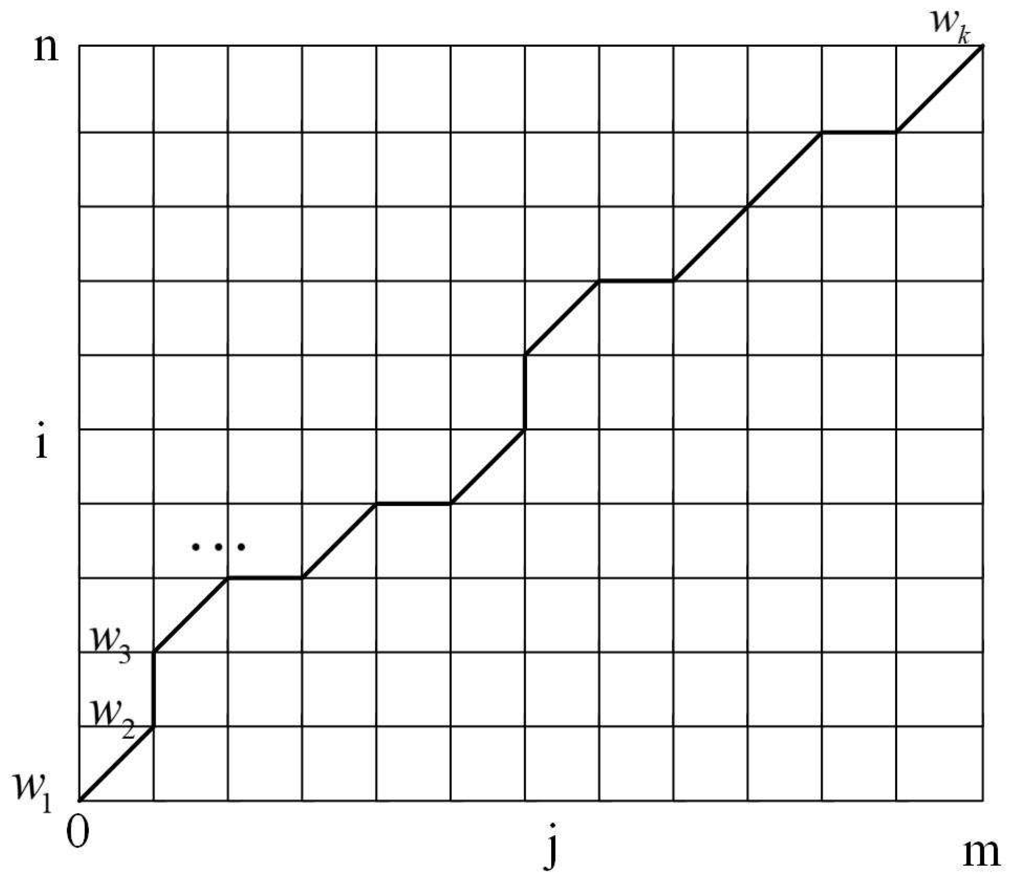
Unlike Euclidean distance, the original intention of DTW is to search a continuous matching relationship, including all points in the two given time series. As shown in Figure 2, the optimal warping path of DTW algorithm represented by W is as follows:

$$W=w_1+w_2+w_3+\cdots +w_k$$

(6)

where $w_h=d_{i,j}$ ($h=1,2,\cdots ,k$, $i=0,1,\cdots ,n$, $j=0,1,\cdots ,m$, and $max(n,m)\le k<n+m-1$). For DTW matching, the following three requirements should be satisfied:

(1)

Boundary conditions: $w_1=d_{1,1}$ and $w_k=d_{n,m}$, indicating that the warping path should start at one corner and end at the other corner in a diagonal direction;

(2)

Continuity condition: each actual warping path should be continuous, that is, if $w_{h-1}=d_{i^{\prime },j^{\prime }}$ and $w_h=d_{i,j}$, then $i-i^{\prime }\le 1$ and $j-j^{\prime }\le 1$.

(3)

Monotonicity condition: neither warping path of two time series should intersects the other, that is, if $w_{h-1}=d_{i^{\prime },j^{\prime }}$ and $w_h=d_{i,j}$, then $i-i^{\prime }\ge 0$ and $j-j^{\prime }\ge 0$.

The task of the DTW algorithm is to search the optimal path by minimizing the warping cost, represented as

$$DTW\left(x_a,x_b\right)=min\left\{\sqrt{{\displaystyle \sum _1^k}{w}_h}/k\right\}$$

(7)

where $DTW(x_a,x_b)$ can be obtained by the recursion provided below and $\gamma (i,j)$ is the total distance of the warping path from the starting point to $d_{i,j}$.

$$\gamma (i,j)=d_{i,j}+min\{\gamma (i-1,j-1),\gamma (i-1,j),\gamma (i,j-1)\}$$

(8)

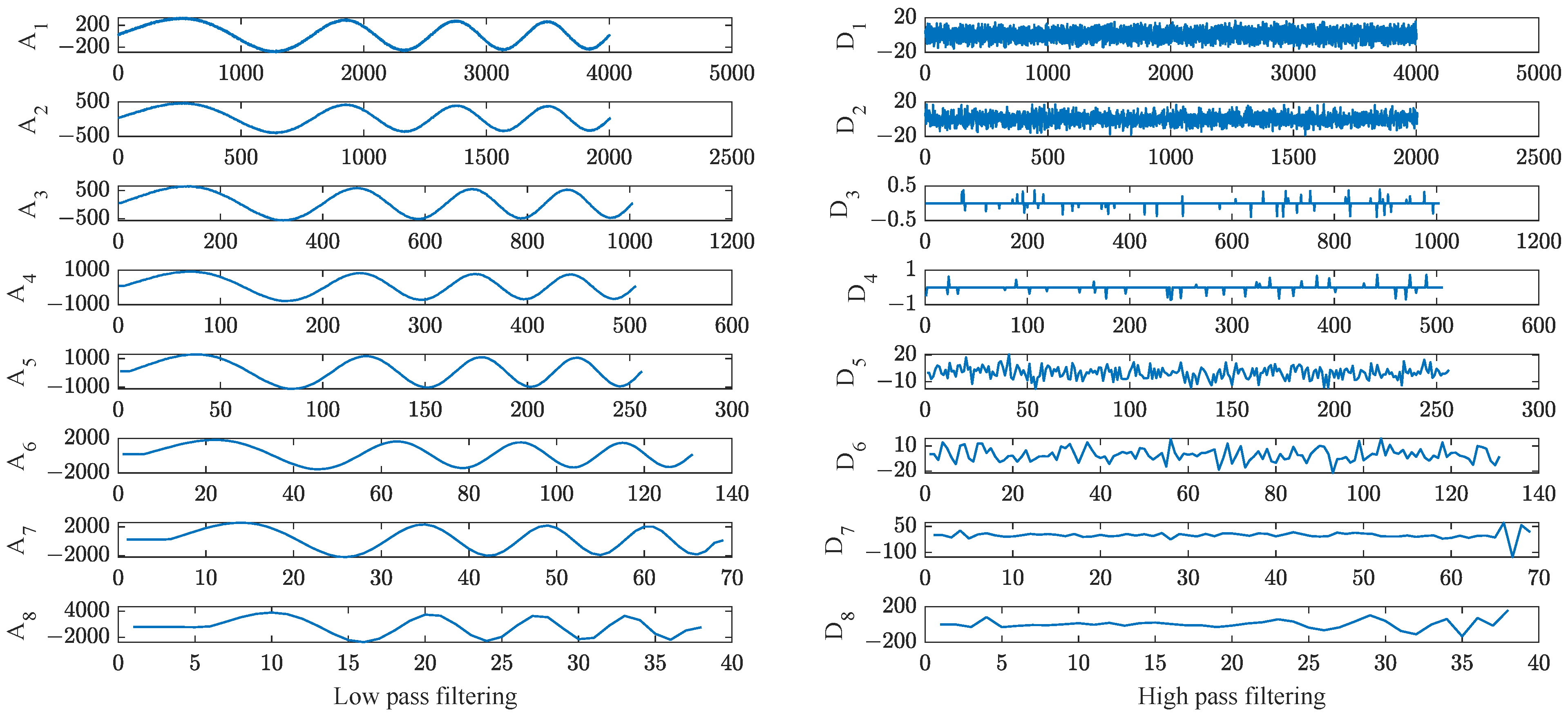
The high-pass filtering (HPF) and low-pass filtering (LPF) comparisons of eight decomposition levels are shown in Figure 3. In the first decomposition level, HPF $D_1$ mainly contains noise, while LPF $A_1$ contains both the data tendency and details of the noise signal. In the second decomposition level, the burst data information in HPF $D_2$ increases significantly, while the noise information is reduced compared with the previous level. Compared with $A_1$, the noise information in $A_2$ is reduced and the data tendency is more obvious. As the number of decomposition levels increases, the noise information included in the HPF becomes less and less, which leads to the DTW distance between the given HPF and the previous one becoming shorter and shorter. However, for the most part only burst data information with no noise exists in HPF under the decomposition case, which results in the DTW distance increasing. According to the above analysis and the relationship between the DTW distance and decomposition levels shown in Figure 4, the optimal decomposition level $j_o$ is chosen as the previous level of the DTW change point.

2.1.2. Noise Threshold Selection

Compared with the optimal selection of decomposition levels, the noise threshold selection is a more important procedure that causes different denoising results directly. An inappropriate noise threshold selection will cause signal distortion, meaning that interference from noise cannot be completely eliminated. The noise coefficients of the detail components are not in a uniform and symmetric distribution, which increases the difficulty of noise reduction. Due to this non-adaptive threshold, the applications of existing threshold selection methods based on noise estimation are not ideal.

The upper and lower noise thresholds ${\lambda }_{j,H}$ and ${\lambda }_{j,L}$ can be denoted as follows:

$$\begin{array}{cc}\hfill {\lambda }_{j,H}& ={\mu }_j+{\kappa }_{j,H}{\sigma }_j\hfill \end{array}$$

(9)

$$\begin{array}{cc}\hfill {\lambda }_{j,L}& ={\mu }_j-{\kappa }_{j,L}{\sigma }_j\hfill \end{array}$$

(10)

where the subscript j represents the number of decomposition levels, ${\kappa }_{j,H}$ and ${\kappa }_{j,L}$ are adjustable parameters related to each threshold, and the mean and standard deviations of the jth decomposition level, ${\mu }_j$ and ${\sigma }_j$, respectively, can be represented as

$$\begin{array}{cc}\hfill {\mu }_j& =\frac{{\sum }_{i=1}^{N_j}{w}_{j,i}}{N_j}\hfill \end{array}$$

(11)

$$\begin{array}{cc}\hfill {\sigma }_j& =\sqrt{\frac{1}{N_j-1}{\displaystyle \sum _{i=1}^{N_j}}{\left(w_{j,i}-{\mu }_j\right)}^2}\hfill \end{array}$$

(12)

where $w_{j,i}$ is the ith element in the detail components $D_j$ and $N_j$ represents the length of $D_j$. The minimum values of the above ${\kappa }_{j,H}$ and ${\kappa }_{j,L}$ can be calculated as

$$\begin{array}{cc}\hfill & {\kappa }_{j,L_{min}}=\frac{{\mu }_j-max\left(\left|w_j<0\right|\right)}{{\sigma }_j}\hfill \end{array}$$

(13)

$$\begin{array}{cc}\hfill & {\kappa }_{j,H_{min}}=\frac{max\left(\left|w_j>0\right|\right)-{\mu }_j}{{\sigma }_j}\hfill \end{array}$$

(14)

where $w_j$ is the element in detail components $D_j$.

In order to obtain an appropriate threshold, the threshold of each decomposition level needs to be designed separately. Meanwhile, the PSR $S_j$ reflecting the sparsity of detail components can be represented as

$$\begin{array}{c}\hfill S_j=\frac{max\left(\left|w_j\right|\right)}{{\sum }_{i=1}^{N_j}\left|w_{j,i}\right|}\end{array}$$

(15)

Furthermore, the threshold selections can be divided into the following three categories:

(1)

$S_j\le 0.01$.

The detail components $D_j$ mainly includes noise. In this case, ${\kappa }_{j,H}={{\kappa }_{j,H}}_{min}$, ${\kappa }_{j,L}={{\kappa }_{j,L}}_{min}$ and all the coefficients of detail components are assigned values of zero.

(2)

$0.01<S_j<T_r$ and $j<j_o$.

The above relationships indicate that detail components $D_j$ include both noise and signal tendency, where $j_o$ represents the optimal decomposition level and $T_r$ is a criterion for distinguishing between the detail components with noise and others without noise, which can be determined as follows [33]:

$$\begin{array}{cc}\hfill {\kappa }_{j,L}& =\left(\frac{S_{r,L}-S_{j,L}}{S_{r,L}}\right){\kappa }_{j,L_{min}}\hfill \end{array}$$

(16)

$$\begin{array}{cc}\hfill {\kappa }_{j,H}& =\left(\frac{S_{r,H}-S_{j,H}}{S_{r,H}}\right){\kappa }_{j,H_{min}}\hfill \end{array}$$

(17)

where $S_{r,L}$ and $S_{j,L}$ are the reference PSR coefficients, and can be defined as follows:

$$\begin{array}{cc}\hfill & S_{r,L}\triangleq \frac{S_{j_o,L}+S_{j_o+1,L}}{2}\hfill \end{array}$$

(18)

$$\begin{array}{cc}\hfill & S_{r,H}\triangleq \frac{S_{j_o,H}+S_{j_o+1,H}}{2}\hfill \end{array}$$

(19)

where $S_{j,L}$ and $S_{j,H}$ are the PSR of the negative and positive coefficients, respectively, and are defined as

$$\begin{array}{c}\hfill S_{j,L}=\frac{max\left(\left|w_j<0\right|\right)}{{\sum }_{i=1}^{N_j}\left|w_{j,i}<0\right|}\end{array}$$

(20)

$$\begin{array}{c}\hfill S_{j,H}=\frac{max\left(\left|w_j\ge 0\right|\right)}{{\sum }_{i=1}^{N_j}\left|w_{j,i}\ge 0\right|}\end{array}$$

(21)

(3)

$S_j\ge T_r$ and $j\ge j_o$.

The above relationships indicate that the number of decomposition levels j has exceeded the optimal number of decomposition levels $j_o$. There is no need to select a noise threshold, as the detail components have no noise in this case.

Remark 1.

According to the methods above derived from [33], the optimal noise thresholds ${\kappa }_{j,H}$ and ${\kappa }_{j,L}$ are chosen. By comparing $T_r$ and $S_j$, it is feasible to determine the number of decomposition levels. However, $T_r$ depends on artificial adjustment, which leads to false judgments as to whether or not the system involves noise. In this paper, an intelligent decomposition level selection scheme is proposed by quantifying the similarity of detail components between the upper and lower levels. In this way, the condition $S_j\ge T_r$ when $j\ge j_o$ can be guaranteed, and incomplete noise reduction due to inaccurate $T_r$ design can be avoided.

2.2. Fault Information Enhancement Technology Based on Continuous Wavelet Transform

The incipient fault of high-speed train traction systems are easily contaminated by noise, as the fault signals are weak in the early stage, and such weak fault information is difficult to extract with traditional fault diagnosis methods. In this paper, a fault information enhancement approach based on the continuous wavelet transform is proposed. The main ideas on how to highlight fault characteristics are expounded as follows.

In the time-frequency space based on the continuous wavelet transform, both frequency domain information and energy change can be monitored. In view of this, the traction system signals of a high-speed train are transformed into the time–frequency domain and the energy change trends are used instead of signal change trends in fault diagnosis analysis. For data with noise reduction ($x_r$), the change trends of signal $T_n(x_r)$ can be obtained by continuous wavelet transform as follows:

$$T_n\left(x_r\right)=\frac{1}{\sqrt{a}}{\int }_{-\infty }^{+\infty }{x}_r(t){\psi }^{*}\left(\frac{t-b}{a}\right)\mathrm{d}t$$

(22)

where ${\psi }^{*}\left(\frac{t-b}{a}\right)$ is the mother wavelet, a is the scaling factor, and b is the translation factor. Further, the energy change trend of the fault data $T_F(x_r)$ can be obtained as

$$T_F(x_r)=T_n(x_r)-T_p(x_r)$$

(23)

where $T_p(x_r)$ is the energy variation trend of the signal. Further, $T_F(x_r)$ can be transformed into fault data $x_F$ containing rich fault information by ICWT (inverse transform of continuous wavelet transform). Based on the above data preprocessing, traction system faults with weak fault characteristics can be diagnosed by combination with existing work on Deep-PCA theories [38].

3. Deep-PCA Based Diagnosability Analysis

According to the noise reduction and fault information enhancement proposed in the previous sections, FNR enhancement-based data preprocessing is realised. For this reason, there is no need to consider the impact of noise in fault detection threshold design, and the sensitivity of the threshold is improved. The proposed approach in this paper is verified in a Deep PCA-based incipient FDD framework, and a diagnosability analysis with Deep-PCA theory is discussed further on the basis of [38].

3.1. Detectability Analysis

The normalized dataset $X\in R^{M\times N}$ (where M is the number of variables that can be measured and N is the number of measurements) can be denoted as

$$X=\overline{X}+\widehat{X}$$

(24)

where $\overline{X}$ represents normal data and $\widehat{X}$ represents fault data.

Implementing SVD (singular value decomposition) on the covariance matrix S of X, we obtain

$$\frac{1}{M-1}X{X}^T=S=P_1{\mathsf{\Lambda }}_{0,1}{P}_1^T$$

(25)

where M represents the number of variables, ${\mathsf{\Lambda }}_{0,1}=diag({\lambda }_{0,1},\cdots ,{\lambda }_{0,M})\in R^{M\times M}$, ${\lambda }_{0,i}(i=1,2,\cdots ,m)$ is the ith eigenvalue of S in descending order, and $P_1\in R^{M\times M}$ is the singular value vector of covariance matrix S.

According to the contribution rate, some singular value vectors are selected to construct $P_{1,1}$ and the remaining part is denoted as $P_{1,2}$, that is, $P_1=\left[P_{1,1},P_{1,2}\right]$. Further, X can be decomposed into two parts, as follows:

$$X=X_{1,1}+X_{1,2}$$

(26)

where

$$\begin{array}{cc}\hfill X_{1,1}& =P_{1,1}{P}_{1,1}^{T}X=P_{1,1}{P}_{1,1}^T(\overline{X}+\widehat{X})\hfill \\ & =P_{1,1}{P}_{1,1}^T\overline{X}+P_{1,1}{P}_{1,1}^T\widehat{X}={\overline{X}}_{1,1}+{\widehat{X}}_{1,1}\hfill \end{array}$$

(27)

$$\begin{array}{cc}\hfill X_{1,2}& =\left(I-P_{1,1}{P}_{1,1}^T\right)X=\left(I-P_{1,1}{P}_{1,1}^T\right)(\overline{X}+\widehat{X})\hfill \\ & =\left(I-P_{1,1}{P}_{1,1}^T\right)\overline{X}+\left(I-P_{1,1}{P}_{1,1}^T\right)\widehat{X}\hfill \\ & ={\overline{X}}_{1,2}+{\widehat{X}}_{1,2}\hfill \end{array}$$

(28)

Similarly, we can obtain

$$X_{j,k}={\overline{X}}_{j,k}+{\widehat{X}}_{j,k}$$

(29)

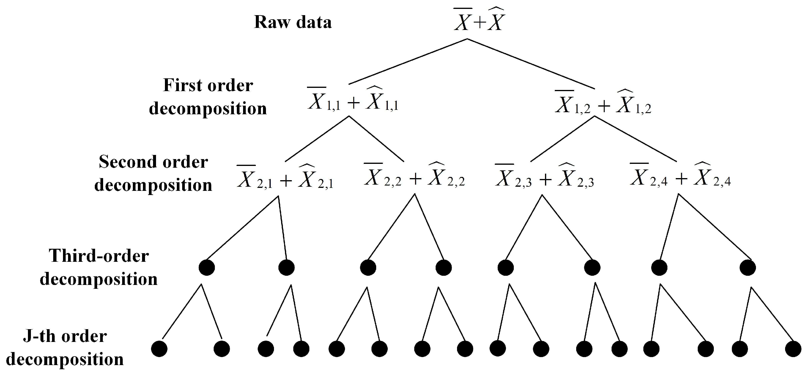
where j represents the number of Deep PCA decomposition levels and $X_{j,k}$ represents the kth data-set of the jth level. Below, the framework of the Deep PCA design and implementation is shown in Figure 5.

The Deep-PCA based fault detection statistics

$$\begin{array}{cc}\hfill T_{j,k}^2=& X^T{P}_{(j+1),(2k-1)}{\mathsf{\Lambda }}_{j,k}^{-1}{P}_{(j+1),(2k-1)}^{T}X\hfill \\ \hfill =& {(\overline{X}+\widehat{X})}^T{P}_{(j+1),(2k-1)}{\mathsf{\Lambda }}_{j,k}^{-1}{P}_{(j+1),(2k-1)}^T(\overline{X}+\widehat{X})\hfill \\ \hfill =& \overline{X}{P}_{(j+1),(2k-1)}{\mathsf{\Lambda }}_{j,k}^{-1}{P}_{(j+1),(2k-1)}^T\overline{X}\hfill \\ \hfill & +\overline{X}{P}_{(j+1),(2k-1)}{\mathsf{\Lambda }}_{j,k}^{-1}{P}_{(j+1),(2k-1)}^T\widehat{X}\hfill \\ \hfill & +\widehat{X}{P}_{(j+1),(2k-1)}{\mathsf{\Lambda }}_{j,k}^{-1}{P}_{(j+1),(2k-1)}^T\overline{X}\hfill \\ \hfill & +\widehat{X}{P}_{(j+1),(2k-1)}{\mathsf{\Lambda }}_{j,k}^{-1}{P}_{(j+1),(2k-1)}^T\widehat{X}\hfill \end{array}$$

(30)

$$\begin{array}{cc}\hfill SP{E}_{j,k}=& \left(I-P_{(j+1),(2k-1)}{P}_{(j+1),(2k-1)}^T\right)X\hfill \\ \hfill =& \left(I-P_{(j+1),(2k-1)}{P}_{(j+1),(2k-1)}^T\right)(\overline{X}+\widehat{X})\hfill \\ \hfill =& \left(I-P_{(j+1),(2k-1)}{P}_{(j+1),(2k-1)}^T\right)\overline{X}\hfill \\ \hfill & +\left(I-P_{(j+1),(2k-1)}{P}_{(j+1),(2k-1)}^T\right)\widehat{X}\hfill \end{array}$$

(31)

where $\overline{X}{P}_{(j+1),(2k-1)}{\mathsf{\Lambda }}_{j,k}^{-1}{P}_{(j+1),(2k-1)}^T\widehat{X}$ are used for the data model involving normal data $\overline{X}$ and fault data $\widehat{X}$. Further, we denote $D_{T^2}(\overline{X},\overline{X})$ as the distance from $\overline{X}$ to the model center of $\overline{X}$, $D_{T^2}(\overline{X},\widehat{X})$ as the distance from $\overline{X}$ to the model center of $\widehat{X}$, and $D_{T^2}(\widehat{X},\widehat{X})$ as the distance from $\widehat{X}$ to the model center of $\widehat{X}$, respectively; here, $\left(I-P_{(j+1),(2k-1)}{P}_{(j+1),(2k-1)}^T\right)\overline{X}$ represents the correlation between the principal components in the dataset $\overline{X}$ (denoted as $R_{SPE}(\overline{X})$) and $\left(I-P_{(j+1),(2k-1)}{P}_{(j+1),(2k-1)}^T\right)\widehat{X}$ represents the correlation between the principal components in the dataset $\widehat{X}$ (denoted as $R_{SPE}(\widehat{X})$). The above formulas can be abbreviated as follows:

$$\begin{array}{cc}\hfill & T_{j,k}^2=D_{T^2}(\overline{X},\overline{X})+2D_{T^2}(\overline{X},\widehat{X})+D_{T^2}(\widehat{X},\widehat{X})\hfill \end{array}$$

(32)

$$\begin{array}{cc}\hfill & SP{E}_{j,k}=R_{SPE}(\overline{X})+R_{SPE}(\widehat{X})\hfill \end{array}$$

(33)

The fault detection logic is as follows:

$$\left\{\begin{array}{cc}{T}^2\le J_{T^2}andSPE\le J_{SPE}\hfill & \mathrm{normal}\hfill \\ Others\hfill & \mathrm{faulty}\hfill \end{array}\right.$$

(34)

where $J_{T^2}$ and $J_{SPE}$ represent the fault detection thresholds of statistics $T^2$ and $SPE$, respectively. In general, the above thresholds correspond to the working conditions of the nominal maximum load of the traction system. Further, we denote the dataset under maximum load working conditions as $\stackrel{=}{X}$ and its corresponding statistics as ${\stackrel{=}{T}}^2=\left({\stackrel{=}{T}}_1^2,{\stackrel{=}{T}}_2^2,{\stackrel{=}{T}}_3^2,\dots ,{{\stackrel{=}{T}}^2}_{\stackrel{=}{N}}\right)$ and $\stackrel{=}{SPE}=\left({\stackrel{=}{SPE}}_1,{\stackrel{=}{SPE}}_2,{\stackrel{=}{SPE}}_3,\dots ,{\stackrel{=}{SPE}}_{\stackrel{=}{N}}\right)$, where $\stackrel{=}{N}$ represents the total number of statistics. Due to the complex and changing environment of train operation and demand for system robustness, the statistics datasets ${\stackrel{=}{T}}^2$ and $\stackrel{=}{SPE}$ can only be obtained by prior conditions. Then, the density function of statistics can be estimated using the KDE (kernel density estimation) function, based on which the corresponding statistic can be used as the detection threshold when the probability is close to 1. In this paper, the KDE functions with Gaussian kernel function are as follows:

$$\begin{array}{c}f\left({\stackrel{=}{T}}^2\right)=\frac{1}{\stackrel{=}{N}h\sqrt{2\pi }}{\displaystyle \sum _{i=1}^{\stackrel{=}{N}}}exp\left\{-\frac{{\left(T_x^2-{\stackrel{=}{T}}_i^2\right)}^2}{2h^2}\right\}\\ f(\stackrel{=}{SPE})=\frac{1}{\stackrel{=}{N}h\sqrt{2\pi }}{\displaystyle \sum _{i=1}^{\stackrel{=}{N}}}exp\left\{-\frac{{\left(SP{E}_x-{\stackrel{=}{SPE}}_i\right)}^2}{2h^2}\right\}\end{array}$$

(35)

where h is the window width (called the smoothing parameter), ${\stackrel{=}{SPE}}_i$ is the ith element in dataset $\stackrel{=}{SPE}$, ${\stackrel{=}{T}}_i^2$ is the ith element in dataset ${\stackrel{=}{T}}^2$, and the subscript x denotes xth element of independent statistics $T_x^2$ and $SP{E}_x$. The probability density functions of the statistics are simulated using the KDE functions shown above. In this paper, the corresponding statistic is selected as the threshold when the probability is 0.98 (denoted as $f_{0.98}^{-1}({\stackrel{=}{T}}^2)$ and $f_{0.98}^{-1}(\stackrel{=}{SPE})$).

$$\begin{array}{cc}\hfill & J_{T^2}=f_{0.98}^{-1}({\stackrel{=}{T}}^2)\hfill \end{array}$$

(36)

$$\begin{array}{cc}\hfill & J_{SPE}=f_{0.98}^{-1}(\stackrel{=}{SPE})\hfill \end{array}$$

(37)

Further, the fault detectability logic under the Deep PCA framework can be obtained as

$$\begin{array}{cc}\hfill & D_{T^2}(\overline{X},\overline{X})+2D_{T^2}(\overline{X},\widehat{X})+D_{T^2}(\widehat{X},\widehat{X})>J_{T^2}\hfill \end{array}$$

(38)

$$\begin{array}{cc}\hfill & R_{SPE}(\overline{X})+R_{SPE}(\widehat{X})>J_{SPE}\hfill \end{array}$$

(39)

According to the Deep-PCA based fault detectability analysis above ($T^2>J_{T^2}orSPE>J_{SPE}$), at least one of the two above conditions should be met.

The geometric description of fault detectability analysis based on a second-order Deep PCA is shown in Figure 6, where the black arrow represents the raw dataset X, the orange arrows represent the first-order decomposition datasets $X_{1,1}$ and $X_{1,2}$, and the dark green arrows represent the second-order decomposition datasets $X_{2,1}$, $X_{2,2}$, $X_{2,3}$, and $X_{2,4}$. Meanwhile, the normal dataset $\overline{x}$ with its decomposition datasets ${\overline{x}}_{2,1}$, ${\overline{x}}_{2,2}$, ${\overline{x}}_{2,3}$, and ${\overline{x}}_{2,4}$ are marked as black dots and the fault dataset $\widehat{x}$ with its decomposition datasets ${\widehat{x}}_{2,1}$, ${\widehat{x}}_{2,2}$, ${\widehat{x}}_{2,3}$, and ${\widehat{x}}_{2,4}$ are marked as red dots.

(1)

Fault detectability analysis based on statistic $T^2$

In the proposed geometric description of detectability analysis, the $T^2$ statistic represents the distance from the dataset to the Deep PCA model center. Supposing the blue dot O in Figure 6 is the center of Deep PCA model, both ${\widehat{x}}_{2,2}$ and ${\widehat{x}}_{2,4}$ are on the extension lines of $X_{2,2}$ and $X_{2,4}$, indicating the incipient fault, as the distance between the dataset and dot O in the normal case has an established range.

(2)

Fault detectability analysis based on statistic $SPE$

Similarly, the $SPE$ statistic represents the degree of correlation between the principal components, which can be simplified as the distance between the two dots in Figure 6. Obviously, both ${\widehat{x}}_{2,2}$ and ${\widehat{x}}_{2,4}$ are on the extension line of $X_{2,2}$ and $X_{2,4}$.

3.2. Isolatability Analysis

In the Deep PCA-based fault isolation scheme, the indicator statistics and corresponding thresholds are extracted in real time to form a fault vector $r^c$, shown as follows:

$$r^c={\left[\frac{T_{j,1}^2}{J_{T^2,j,1}}\frac{SP{E}_{j,1}}{J_{SPE,j,1}}\cdots \frac{T_{j,2^j}^2}{J_{T^2,j,2^j}}\frac{SP{E}_{j,2^j}}{J_{SPE,j,2^j}}\right]}^T$$

(40)

where $r^c$ represents the feature vector of the cth fault, j represents the number of Deep-PCA decomposition levels, $T_{j,k}^2$ and $SP{E}_{j,k}$ represent the two statistics of dataset $X_{j,k}$, and $J_{T^2,j,k}$ and $J_{SPE,j,k}$ are the corresponding thresholds of $T_{j,k}^2$ and $SP{E}_{j,k}$. Further, the vector p is obtained by projecting the fault eigenvector $r^c$ onto the interval $\left[0.5,1\right)$.

$$\begin{array}{c}\hfill p_k=\frac{1}{1+exp(-(r_k^c))},(k=1,2,...,2^j)\end{array}$$

(41)

$$\begin{array}{c}\hfill p={[p_1,p_2,\dots p_k]}^T\end{array}$$

(42)

where $r_k^c$ represents the kth element of $r^c$. Assuming that $N_c$ groups of fault data with $N_c$ vectors p are obtained under the cth fault case, a fault characteristic matrix $P^c$ is formed by vectors p in columns, and its corresponding mean vector ${\mu }^c$ and covariance matrix ${\mathsf{\Sigma }}^c$ are as follows:

$$\begin{array}{cc}\hfill {\mu }_d^c& =\frac{1}{N_c}\sum _{b=1}^{N_c}{P}_{d,b}^c\hfill \\ \hfill {\mu }^c& ={\left[{\mu }_1^c,{\mu }_2^c,\dots {\mu }_8^c\right]}^T\hfill \end{array}$$

(43)

$$\begin{array}{cc}\hfill {\mathsf{\Sigma }}^c& =\frac{1}{N_c}\left(P^c-I{\mu }^c\right){\left(P^c-I{\mu }^c\right)}^T\hfill \end{array}$$

(44)

where $P_{d,b}^c$ is the bth element of the dth row of $P^c$, ${\mu }_d^c$ is the mean of the dth row of matrix $P^c$, and I is the identity matrix. Further, the KLD (Kullback–Leibler Distance) between the real-time feature matrix $P^c$ and fault characteristic matrix ${\tilde{P}}^c$ can be represented as

$$\begin{array}{cc}\hfill & K(P^c,{\tilde{P}}^c)=\frac{1}{2}tr\left[{({\mathsf{\Sigma }}^c)}^{-1}{\tilde{\mathsf{\Sigma }}}^c+{({\tilde{\mathsf{\Sigma }}}^c)}^{-1}{\mathsf{\Sigma }}^c-2\times I_{2^j\times 2^j}\right]\hfill \\ \hfill & +\frac{1}{2}{\left({\mu }^c-{\tilde{\mu }}^c\right)}^T\left({({\mathsf{\Sigma }}^c)}^{-1}+{({\tilde{\mathsf{\Sigma }}}^c)}^{-1}\right)\left({\mu }_{-}^c{\tilde{\mu }}^c\right)\hfill \end{array}$$

(45)

In conclusion, the incipient fault can be isolated under the Deep PCA framework if and only if

$${({\mathsf{\Sigma }}^c)}^{-1}\mathrm{exists}.$$

(46)

Furthermore, we have the following fault isolation logic.

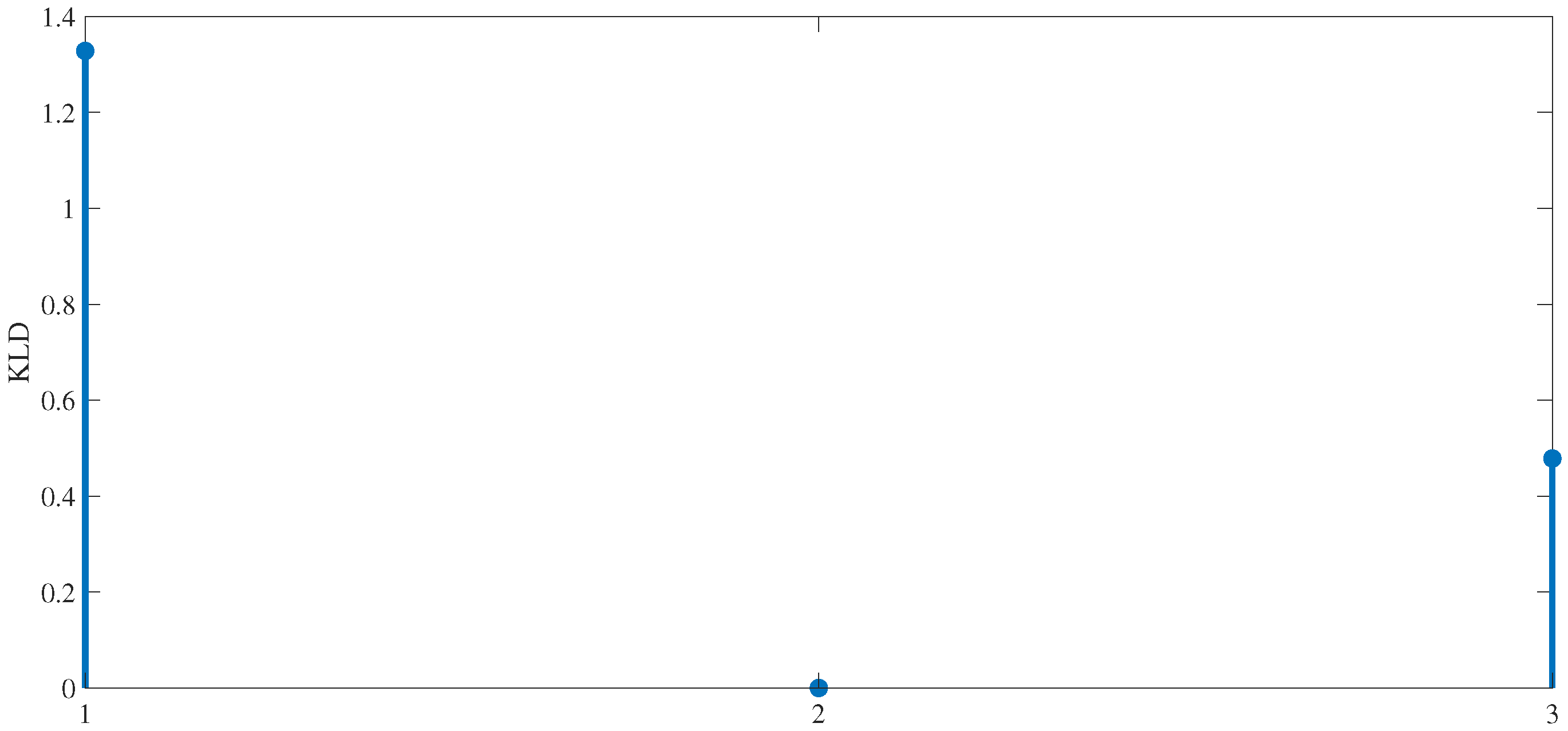
It is assumed that Q types of fault characteristic matrices $\widetilde{P^i}(i=1,\cdots ,Q)$ exist. The distance between $P^c$ and the corresponding fault characteristic matrix $\widetilde{P^i}$ can be obtained using Formula (45), and the minimum value can be represented as

$$D{K}_l=min\{K(P^c,\widetilde{P^1}),\cdots ,K(P^c,\widetilde{P^Q})\}$$

(47)

$D{K}_l\le J_{th}$ indicates the occurrence of fault $\widetilde{P^l}$, where $J_{th}$ is the KLD threshold of the corresponding fault type.

4. Experimental Verification

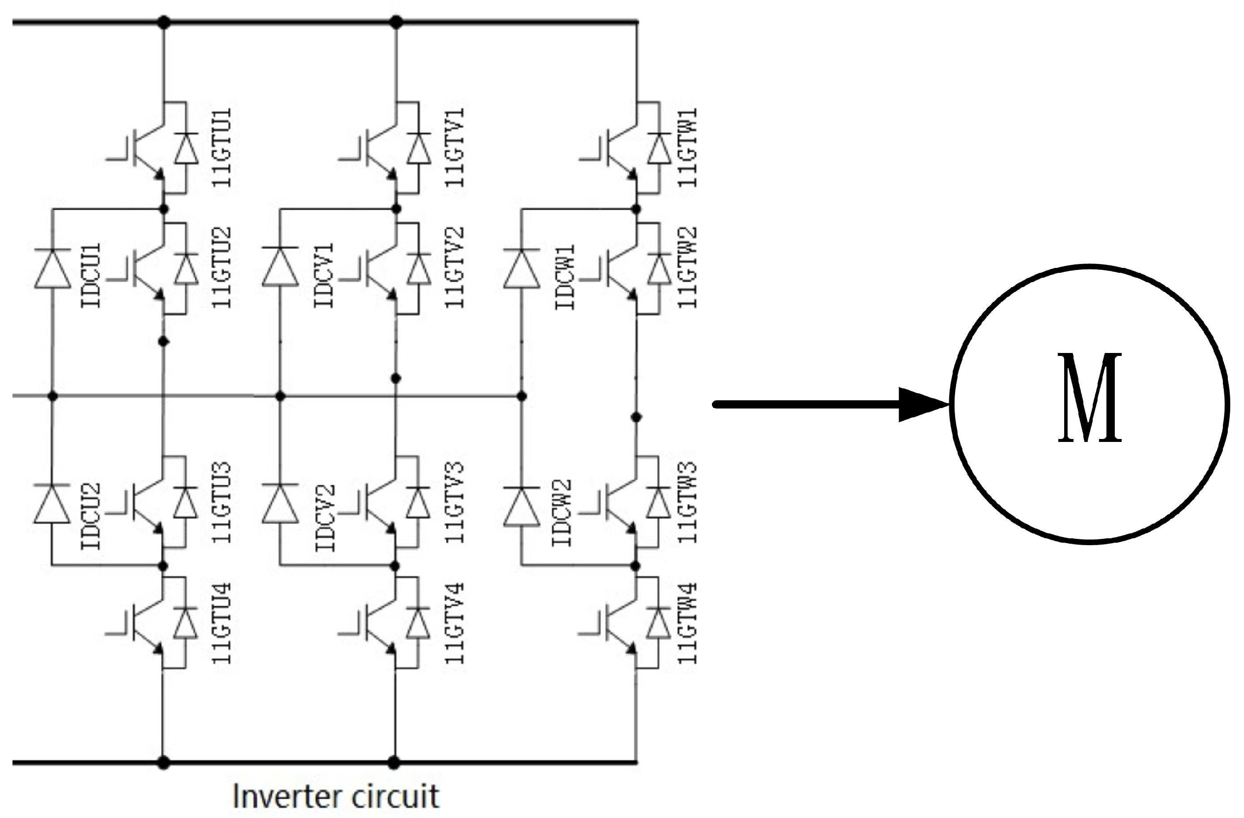
In this study, real time simulation data for a high-speed train running were derived from the TDCS-FIB (Traction Drive Control System–Fault Injection Benchmark) platform, shown as Figure 7. Three types of incipient faults (motor bearing faults, sensor drift faults, and periodic faults on the inverter circuit) containing noise signals were considered, as shown in

Table 1. Fault injection.

Number	Type	Time
$f_1$	Incipient bearing fault on induction motor	$1\times {10}^5$ sampling time
$f_2$	Incipient drift fault on inverter sensors	$1\times {10}^5$ sampling time
$f_3$	Incipient periodic fault on inverter circuit	$1\times {10}^5$ sampling time

.

4.1. Experimental Results for FNR Enhancement-Based Data Preprocessing

According to the FNR signal enhancement theories proposed in the sections above, the data preprocessing results are shown in the following sections, including noise reduction and fault information enhancement of the current signal. In particular, to show the noise reduction results in detail, 8000 samples near the fault injection instant are chosen.

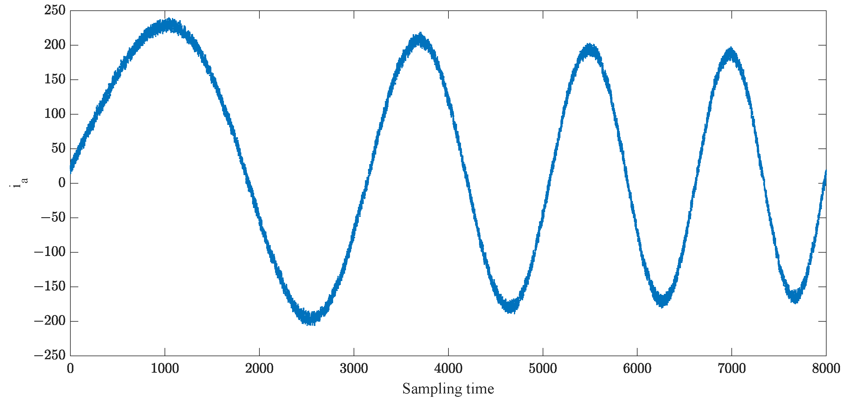
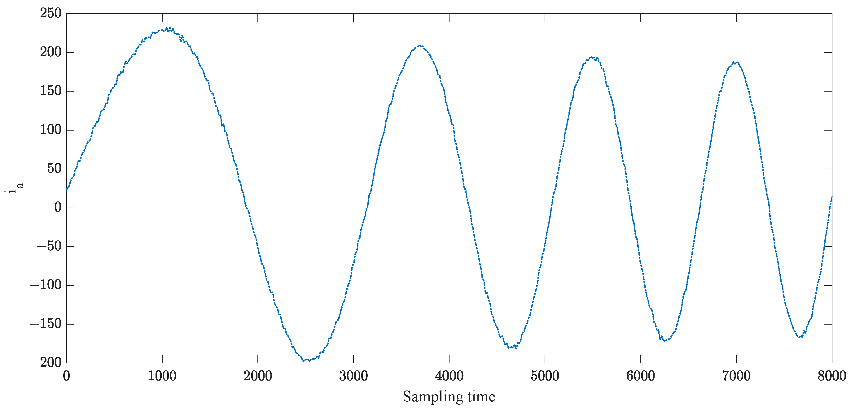
Taking $i_a$ as an example, the raw data of the current signal $i_a$ with noise is shown in Figure 8. Due to the weak characteristics of incipient faults in the early stage, random noise causes high numbers of false alarms and missed alarms. The experimental results for current signal $i_a$ with noise reduction are shown in Figure 9, in which the tendency is obvious and the prominent perturbation is removed. According to further analysis of the experimental results, the noise reduction effect depends on the number of decomposition levels and the noise threshold selection. In this paper, an intelligent decomposition level selection scheme is proposed by quantifying the distance between high-pass filters. The threshold design using the peak–sum ratio and intelligent decomposition-based $T_r$ selection improves the noise reduction performance even further.

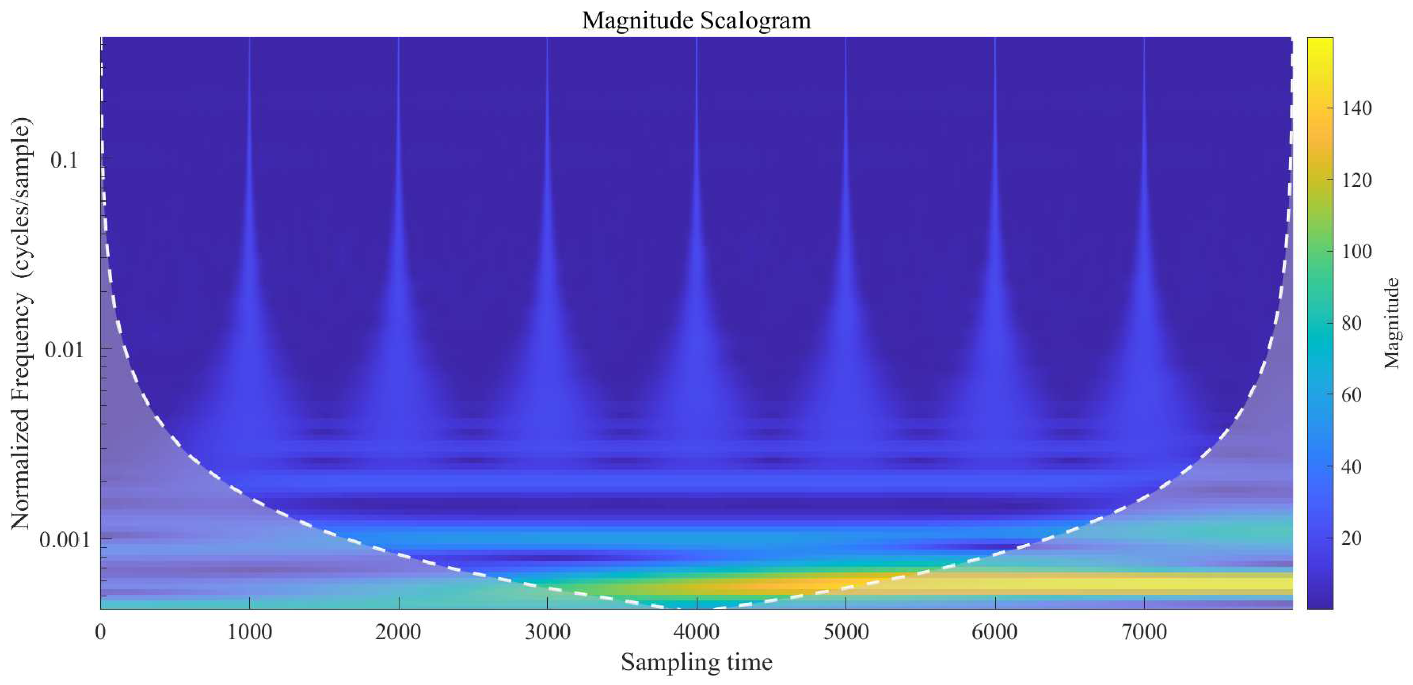
Analyzing the data trend from the viewpoint of energy is one of the main innovations of this article. Based on continuous wavelet transform, the time-frequency domain property of current signal $i_a$ is shown in Figure 10, where the yellow region denotes high energy and the blue region denotes low energy. By comparing the periods before and after the fault instant, it is clear that the energy band drifts upward. The time–frequency domain property of current signal $i_a$ with the normal trend removed is shown in Figure 11. The energy band color before fault injection instantly changes from yellow to blue, which indicates even further the obvious fault trend that can be obtained using continuous wavelet transform to extract the normal data trend and remove the normal trend of the fault data in real time.

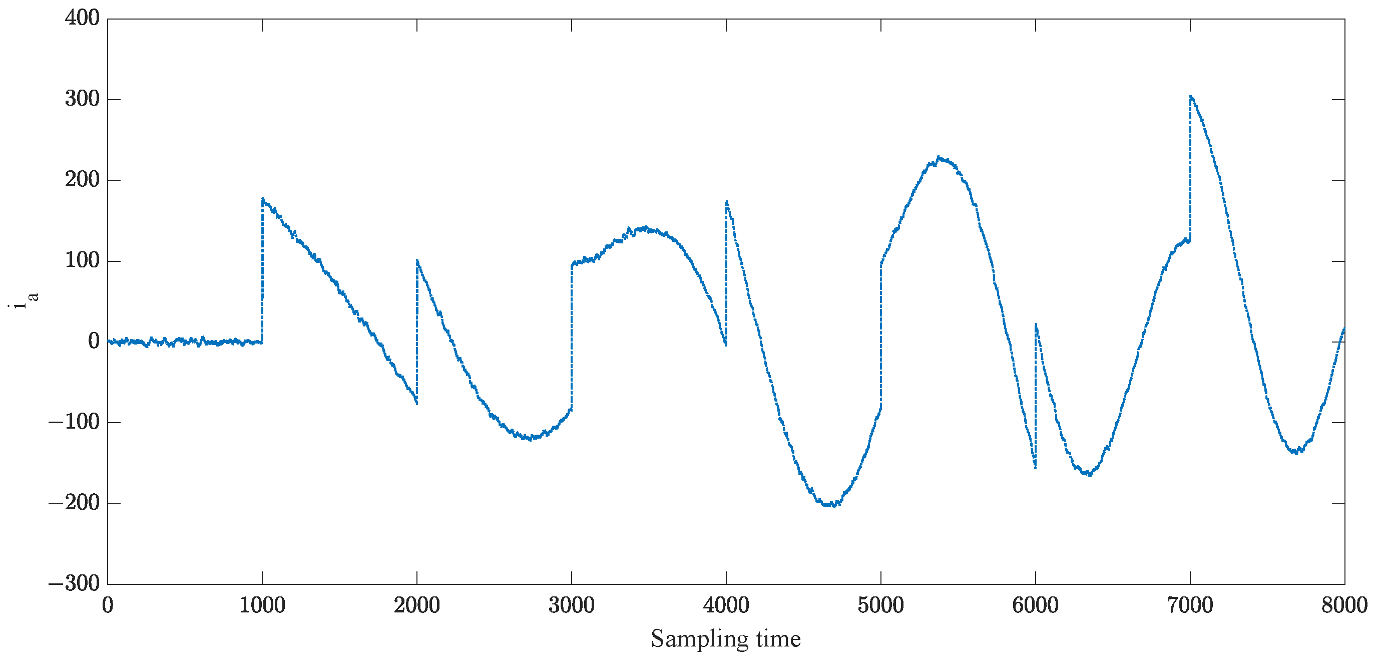
For the time-frequency domain property of current signal $i_a$ with the normal trend removed to the original dataset dimension, the current signal $i_a$ in the time domain with FNR enhancement is shown in Figure 12. In particular, the sudden change in Figure 12 is related to the raw dataset and fault injection instant, which indicate that the current residuals cannot be used as a fault detection indicator directly. Therefore, the current data with FNR enhancement, including noise reduction and fault information enhancement, can be used as the actual dataset for fault detection. Related experimental results on fault detection and isolation in combination with the Deep PCA-based incipient fault diagnosis scheme are shown in the following sections.

4.2. Fault Detection and Isolation

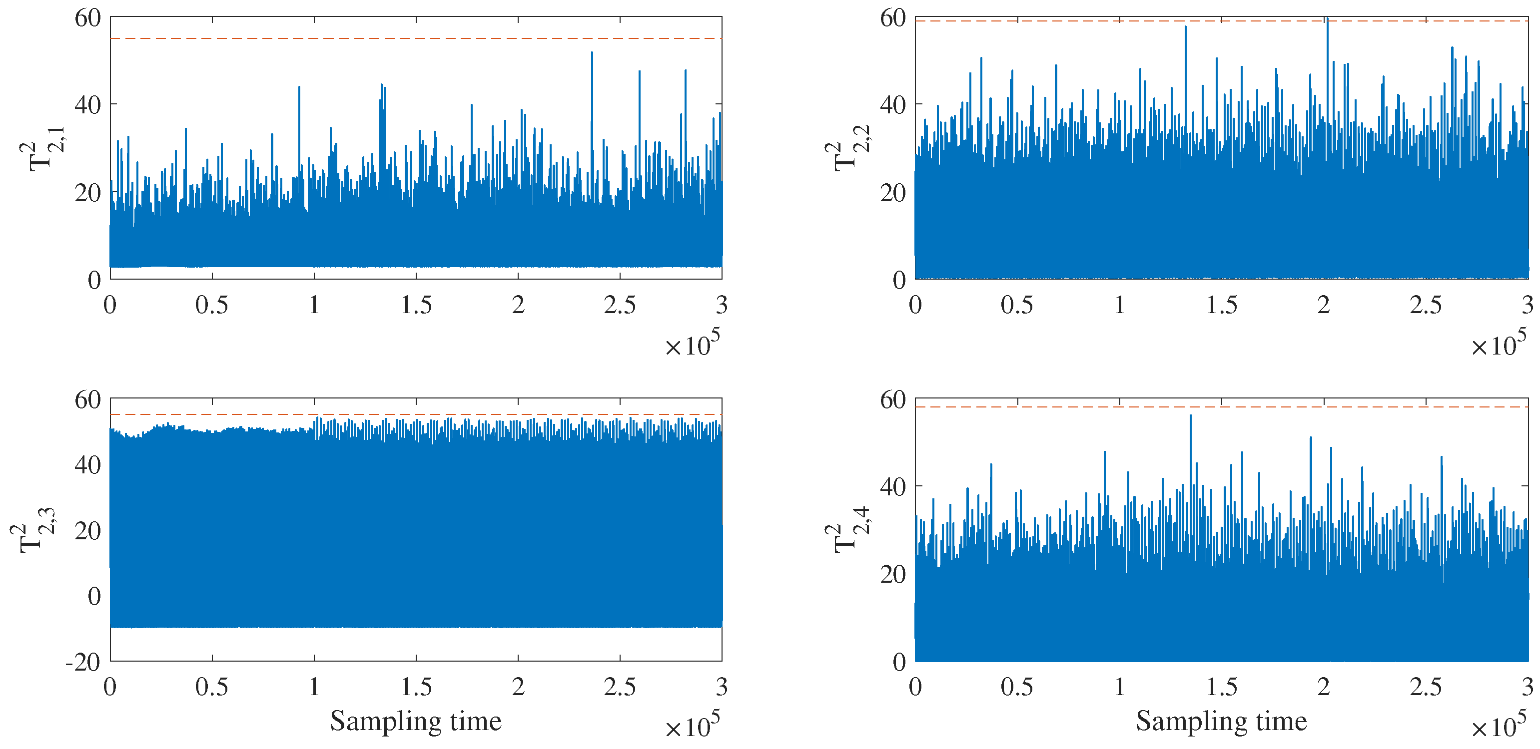
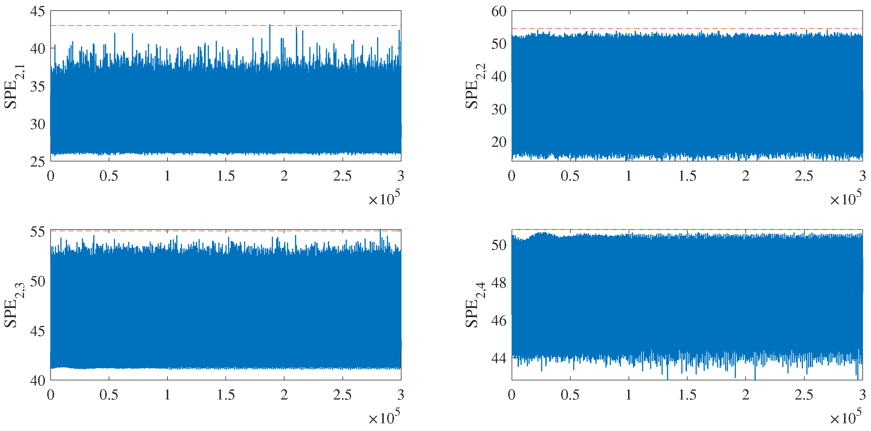
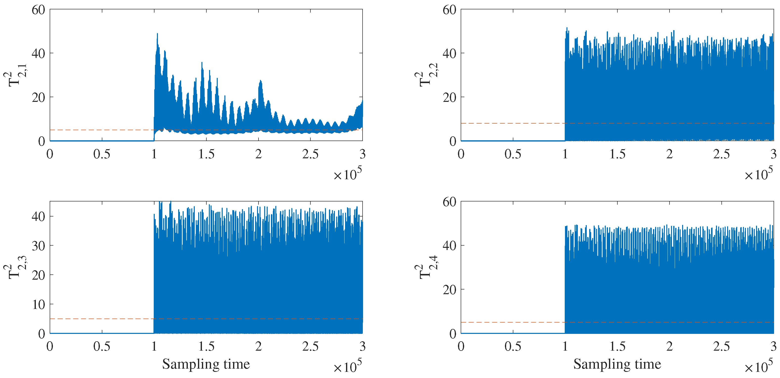
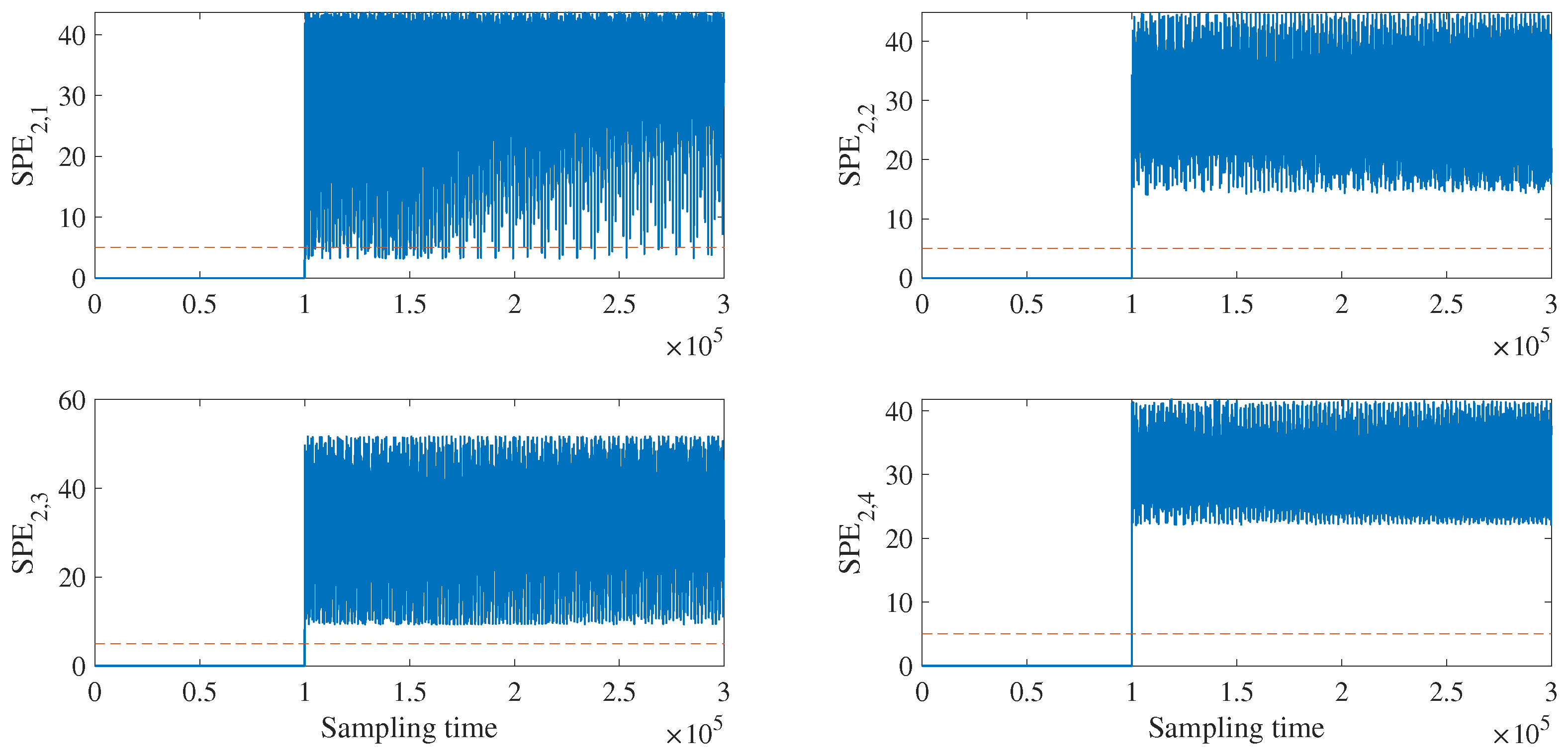
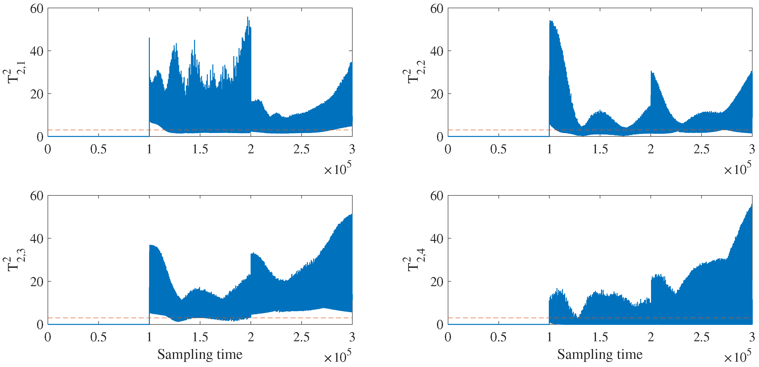
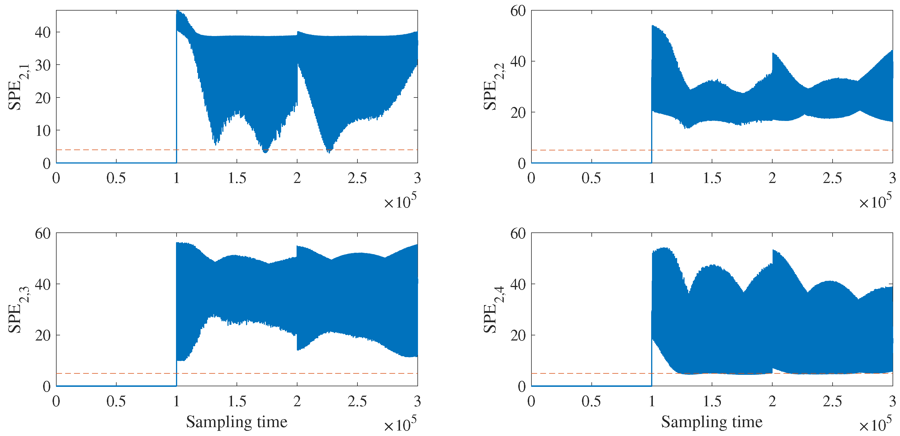
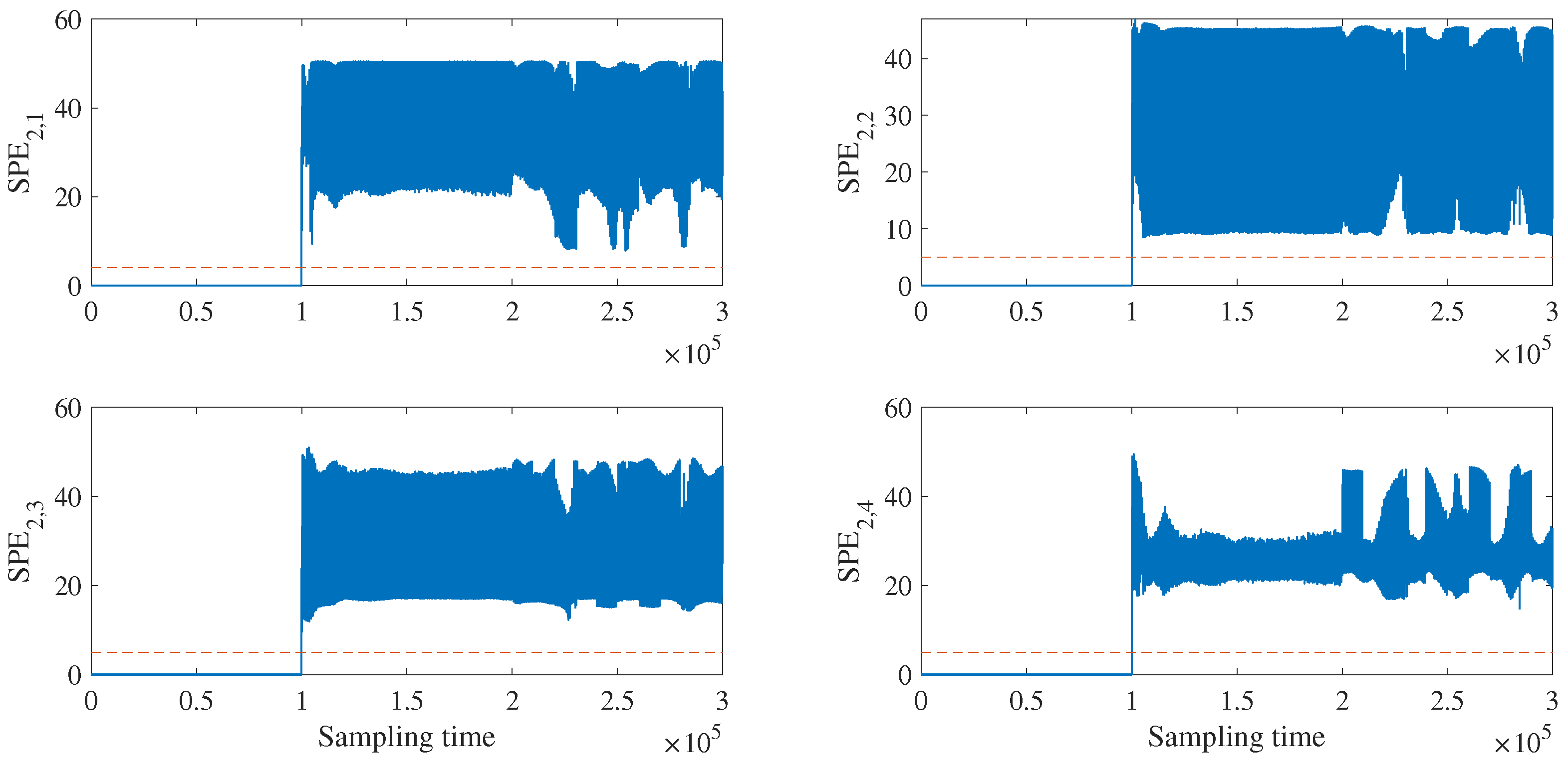
According to the experimental results in this section based on FNR enhancement of the current signal in a high-speed train traction system, better incipient fault detection and isolation performance can be achieved under the Deep PCA framework. Taking a second-order Deep PCA model as an example, four datasets ($X_{2,1}$, $X_{2,2}$, $X_{2,3}$, and $X_{2,4}$) and eight statistics ($T_{2,1}^2$, $T_{2,2}^2$, $T_{2,3}^2$, $T_{2,4}^2$, $SP{E}_{2,1}$, $SP{E}_{2,2}$, $SP{E}_{2,3}$, and $SP{E}_{2,4}$) were obtained. In the following experimental result analysis, the blue lines represent the statistic residuals and the red lines represent the corresponding thresholds. Meanwhile, the fault detection and isolation comparisons between the raw data and data with FNR enhancement are provided to illustrate the effectiveness of the proposed data preprocessing and Deep PCA-based incipient fault diagnosis scheme.

4.2.1. Fault Detection and Isolation of Raw Data

Taking the raw data on incipient bearing faults in the induction motor ($f_1$ in Table 1) containing noise as an example, both Figure 13 and Figure 14 show the experimental results on Deep PCA-based fault detection for the raw data. Obviously, neither the $T^2$ nor the $SPE$ statistics can achieve relatively ideal detection performance, which results in high error rates in isolation, as fault isolation is the next step in fault detection in the Deep PCA-based fault diagnosis framework.

4.2.2. Fault Detection and Isolation for Data with FNR Enhancement

The fault detection and isolation results for fault data including incipient bearing faults on induction motor ($f_1$), incipient drift faults on inverter sensors ($f_2$), and incipient periodic faults on inverter circuit ($f_3$) with FNR enhancement are shown in the following section. Furthermore, comparisons with the raw data case and related analysis are provided at the same time.

The experimental results of Deep PCA-based fault detection for $f_1$, $f_2$, and $f_3$ with FNR enhancement are shown in Figure 15, Figure 16, Figure 17, Figure 18, Figure 19 and Figure 20. According to the responses of statistics $T_{2,1}^2$, $T_{2,2}^2$, $T_{2,3}^2$, $T_{2,4}^2$, $SP{E}_{2,1}$, $SP{E}_{2,2}$, $SP{E}_{2,3}$, and $SP{E}_{2,4}$, the three kinds of incipient traction system faults considered in this paper can be detected in a timely fashion.

Remark 2.

Compared with the $SPE$ statistic, $T^2$ is more sensitive to incipient faults. Compared with fault the detection results for the raw data, a higher fault detection sensitivity and fault identification capability is obtained with FNR enhancement-based data preprocessing technology. Furthermore, taking the weak periodical fault signal $f_3$ as an example, the existing Deep PCA-based incipient fault detection scheme [38] only issues alarms when the fault amplitude increases. According to the experimental results shown in Figure 19 and Figure 20, this problem can be solved by the data preprocessing method based on FNR enhancement from the perspective of fault energy.

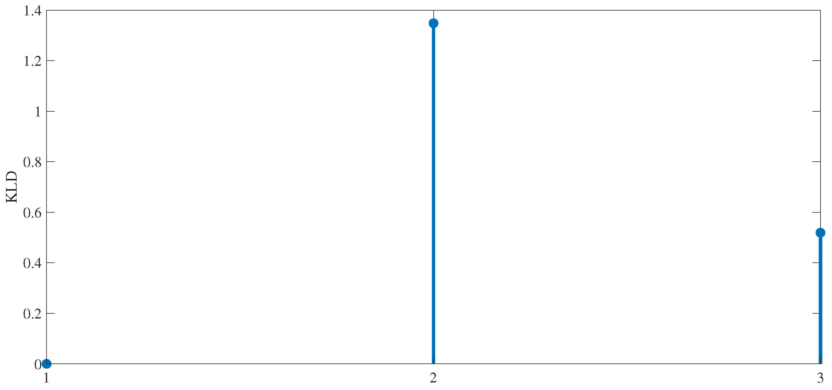
According to the isolatability analysis proposed in this paper, incipient faults can be isolated under the Deep PCA framework if and only if ${({\mathsf{\Sigma }}^c)}^{-1}\mathrm{exists}$. In the experimental results on fault isolation,

$${\left({\mathsf{\Sigma }}_{f_1}^c\right)}^{-1}=\left[\begin{array}{cccccccc}a& b& c& c& -a& -b& -c& -c\\ b& d& -e& -e& -b& -d& e& e\\ c& -e& f& -g& -c& e& -f& g\\ c& -e& -g& f& -c& e& g& -f\\ -a& -b& -c& -c& a& b& c& c\\ -b& -d& e& e& b& d& -e& -e\\ -c& e& -f& g& c& -e& f& -g\\ -c& e& g& -f& c& -e& -g& f\end{array}\right]$$

(48)

where $a=1.91\times {10}^{17}$; $b=8.81\times {10}^{16}$; $c=8.00\times {10}^{16}$; $d=1.33\times {10}^{17}$; $e=6.69\times {10}^{16}$; $f=1.49\times {10}^{17}$; $g=8.21\times {10}^{16}$.

$${\left({\mathsf{\Sigma }}_{f_2}^c\right)}^{-1}=\left[\begin{array}{cccccccc}-a& b& c& -d& a& -b& -c& d\\ b& e& -f& -g& -b& -e& f& g\\ c& -f& -b& -a& -c& f& b& a\\ -d& -g& -a& e& d& g& a& -e\\ a& -b& -c& d& -a& b& c& -d\\ -b& -e& f& g& b& e& -f& -g\\ -c& f& b& a& c& -f& -b& -a\\ d& g& a& -e& -d& -g& -a& e\end{array}\right]$$

(49)

where $a=1.79\times {10}^{17}$; $b=2.16\times {10}^{16}$; $c=9.65\times {10}^{16}$; $d=1.91\times {10}^{17}$; $e=9.05\times {10}^{16}$; $f=1.15\times {10}^{17}$; $g=8.07\times {10}^{16}$.

$${\left({\mathsf{\Sigma }}_{f_3}^c\right)}^{-1}=\left[\begin{array}{cccccccc}-a& b& -c& -c& a& -b& c& c\\ b& -d& -e& -e& -b& d& e& e\\ -c& -e& f& -g& c& e& -f& g\\ -c& -e& -g& f& c& e& g& -f\\ a& -b& c& c& -a& b& -c& -c\\ -b& d& e& e& b& -d& -e& -e\\ c& e& -f& g& -c& -e& f& -g\\ c& e& g& -f& -c& -e& -g& f\end{array}\right]$$

(50)

where $a=1.56\times {10}^{17}$; $b=1.53\times {10}^{16}$; $c=6.55\times {10}^{16}$; $d=5.71\times {10}^{16}$; $e=3.95\times {10}^{16}$; $f=8.81\times {10}^{16}$; $g=1.42\times {10}^{17}$. In the above representations, ${\mathsf{\Sigma }}_{f_1}^c$, ${\mathsf{\Sigma }}_{f_2}^c$, and ${\mathsf{\Sigma }}_{f_3}^c$ are the covariance matrices corresponding to $f_1$, $f_2$, and $f_3$, respectively. Further, the Deep PCA-based and KLD-based fault isolation results for $f_1$, $f_2$, and $f_3$ with FNR enhancement are shown in Figure 21, Figure 22 and Figure 23. The simulation results show the effectiveness and feasibility of the proposed Deep PCA-based isolatability analysis, while the proposed FNR enhancement-based data preprocessing approach can further improve the accuracy of incipient fault isolation.

5. Conclusions

In this paper, an FNR enhancement scheme including noise reduction based on discrete wavelet transform and fault information enhancement based on continuous wavelet transform is proposed, then applied to Deep PCA-based incipient fault diagnosis of a high-speed railway traction system. The contributions of this paper can be summarized as follows: (1) an intelligent decomposition level selection scheme is proposed by quantifying the similarity of detail components; (2) selection of the noise threshold is determined and optimized to further improve the accuracy of noise reduction; (3) a continuous wavelet transform-based fault information enhancement approach is proposed from the perspective of fault energy; (4) a diagnosability analysis under the Deep PCA framework is provided using geometric descriptions.

References

1. Chen, H.T.; Jiang, B. A review of fault detection and diagnosis for the traction system in high-speed trains. IEEE Trans. Intell. Transp. Syst. 2020, 21, 450–465. [Google Scholar] [CrossRef]
2. Chen, H.T.; Jiang, B.; Ding, S.X.; Huang, B. Data-driven fault diagnosis for traction systems in high-speed trains: A survey, challenges, and perspectives. IEEE Trans. Intell. Transp. Syst. 2022, 23, 1700–1716. [Google Scholar] [CrossRef]
3. Yu, W.K.; Zhao, C.H.; Huang, B. MoniNet with concurrent analytics of temporal and spatial information for fault detection in industrial processes. IEEE Trans. Cybern. 2021, 52, 8340–8351. [Google Scholar] [CrossRef] [PubMed]
4. Yu, W.K.; Zhao, C.H.; Huang, B. Recursive cointegration analytics for adaptive monitoring of nonstationary industrial processes with both static and dynamic variations. J. Process. Control. 2020, 92, 319–332. [Google Scholar] [CrossRef]
5. Cai, T.; Silverman, B.W. Incorporating information on neighbouring coefficients into wavelet estimation. Sankhy. Indian. J. Statist. B 2001, 63, 127–148. [Google Scholar]
6. Messer, S.R.; Agzarian, J.; Abbott, D. Optimal wavelet denoising for phonocar diograms. Microelectron. J. 2001, 32, 931–941. [Google Scholar] [CrossRef]
7. Ali, M.N.; Dahshan, E.l.; Yahia, E.A. Denoising of Heart Sound Signals Using Discrete Wavelet Transform. Circuits Syst. Signal. Process. 2017, 36, 4482–4497. [Google Scholar] [CrossRef]
8. Dawid, G.; Grzegorz, R.L. Wavelet-based denoising method for real phonocardiography signal recorded by mobile devices in noisy environment. Comput. Biol. Med. 2014, 52, 119–129. [Google Scholar]
9. Jiang, J.; Guo, J.; Fan, W.; Chen, Q. An improved adaptive wavelet denoising method based on neighboring coefficients. In Proceedings of the 2010 8th World Congress on Intelligent Control and Automation, Jinan, China, 7–9 July 2010; Volume 10, pp. 2894–2898. [Google Scholar]
10. Patil, P.B.; Chavan, M.S. A wavelet based method for denoising of biomedical signal. In Proceedings of the International Conference on Pattern Recognition, Informatics and Medical Engineering (PRIME-2012), Salem, India, 21–23 March 2012; Volume 10, pp. 278–283. [Google Scholar]
11. Rao, B.C.; Latha, M.M. Selective neighbouring wavelet coefficients approach for image denoising. Int. J. Commun. Syst. 2011, 2, 73–77. [Google Scholar]
12. Qin, X.W.; Yue, Y.; Dong, X.G. An improved method of image denoising based on wavelet transform. In Proceedings of the 2010 International Conference on Computer, Mechatronics, Control and Electronic Engineering, Changchun, China, 24–26 August 2010; Volume 10, pp. 167–170. [Google Scholar]
13. Golroudbari, M.A. Signal denoising based on wavelet transform using a multi-level threshold function. In Proceedings of the 2013 7th International Conference on Application of Information and Communication Technologies, Baku, Azerbaijan, 23–25 October 2013; Volume 7, pp. 1–5. [Google Scholar]
14. Chen, G.Y.; Bui, T.D. Multiwavelets denoising using neighboring coefficients. IEEE Signal. Process. Lett 2003, 10, 211–214. [Google Scholar] [CrossRef]
15. Om, H.; Biswas, M. A generalized image denoising method using neighbouring wavelet coefficients. Signal Image Video Process. 2015, 9, 191–200. [Google Scholar] [CrossRef]
16. Yang, G.R.G.; Ren, M.W. RETRACTED: Wavelet denoising using principal component analysis. Exp. Sys. App. 2011, 38, 1073–1076. [Google Scholar] [CrossRef]
17. Chen, G.Y.; Kegl, B. Image denoising with complex ridgelets. Artif. Neural Netw. Pattern. Recognit. 2007, 40, 578–585. [Google Scholar] [CrossRef]
18. Om, H.; Biswas, M.T. An Improved Image Denoising Method Based on Wavelet Thresholding. J. Signal Inf. Process. 2012, 1, 8–28. [Google Scholar] [CrossRef] [Green Version]
19. Zhou, D.; Cheng, W. Image denoising with an optimal threshold and neighbouring window. Pattern Recognit. Lett. 2008, 29, 1694–1697. [Google Scholar]
20. Cetin, A.E.; Tofighi, M. Projection-based wavelet denoising. IEEE Signal. Process. Mag. 2015, 32, 120–124. [Google Scholar] [CrossRef]
21. Zhao, R.M.; Cui, H.M. Improved threshold denoising method based on wavelet transform. In Proceedings of the 2015 7th International Conference on Modelling, Identification and Control (ICMIC), Sousse, Tunisia, 18–20 December 2015; Volume 10, pp. 1–4. [Google Scholar]
22. Biswas, M.; Om, H. An image denoising threshold estimation method. Choice 2013, 1000, 2l. [Google Scholar]
23. Madhu, S.; Bhavani, H.B.; Sumathi, S.; Vidya, H.A. A novel algorithm for denoising of simulated partial discharge signals using adaptive wavelet thresholding methods. In Proceedings of the 2015 2nd International Conference on Electronics and Communication Systems (ICECS), Coimbatore, India, 26–27 February 2015; Volume 10, pp. 1596–1602. [Google Scholar]
24. Madadi, Z.; Anand, G.V.; Premkumar, A.B. Signal detection in generalized Gaussian noise by nonlinear wavelet denoising. IEEE Trans. Circuits Syst. I Reg. Papers 2013, 11, 2973–2986. [Google Scholar] [CrossRef]
25. Madhu, S.; Bhavani, H.B.; Umathi, S.S. Performance analysis of thresholding techniques for denoising of simulated partial discharge signals corrupted by Gaussian white noise. In Proceedings of the 2015 International Conference on Power and Advanced Control Engineering (ICPACE), Bangalore, India, 12–14 August 2015; Volume 10, pp. 399–404. [Google Scholar]
26. Tyagi, B.; Vidya, H.A. Application of Wavelet Shrinkage Denoising Method Based on Genetic Algorithm to Partial Discharge Signals. In Proceedings of the International Conference on VLSI, Communication, Advanced Devices, Signals & Systems and Networking (VCASAN-2013), Bangalore, India, 17–19 July 2013; Springer: New Delhi, India, 2013; Volume 258, pp. 142–149. [Google Scholar]
27. Hamadi, S.H.K.; Isa, M.; Ishak, L.M.; Rohani, M.N.K.H.; Yii, C.C.; Ismail, B.; Shafiq, M. Evaluation of denoising performance indices for noisy partial discharge signal based on DWT technique. In Proceedings of the 2017 IEEE 15th Student Conference on Research and Development (SCOReD), Wilayah Persekutuan Putrajaya, Malaysia, 13–14 December 2017; Volume 5, pp. 392–397. [Google Scholar]
28. Hussein, R.; Shaban, K.B.; El-Hag, A.H. Histogram-based thresholding in discrete wavelet transform for partial discharge signal denoising. In Proceedings of the 2015 International Conference on Communications, Signal Processing, and their Applications (ICCSPA’15), Sharjah, United Arab Emirates, 17–19 February 2015; Volume 10, pp. 1–5. [Google Scholar]
29. Guo, S.; Wu, F.; Wei, W.; Guo, J.; Ji, Y.; Wang, Y. A novel wavelet denoising method used for droplet volume detection in the microfluidic system. In Proceedings of the 2013 IEEE International Conference on Mechatronics and Automation, Takamatsu, Japan, 4–7 August 2013; Volume 10, pp. 1732–1737. [Google Scholar]
30. Weil, W.; Guo, S.; Wu, F.; Ji, Y.; Wang, Y. Image processing-based measurement of volume for droplets in the microfluidic system. In Proceedings of the 2013 ICME International Conference on Complex Medical Engineering, Beijing, China, 25–28 May 2013; Volume 10, pp. 518–522. [Google Scholar]
31. Xie, X.Y.; Liu, Y.; Lin, X.M.; Wang, H. The application of adaptive step threshold method in fluorescence signal detection. In Proceedings of the 2017 2nd IEEE International Conference on Computational Intelligence and Applications (ICCIA), Beijing, China, 8–11 September 2017; Volume 10, pp. 411–416. [Google Scholar]
32. Huang, C.; Xia, G.; Jin, S.; Hu, M.; Wu, S.J. Denoising analysis of compact CCD-based spectrometer. Optik 2018, 157, 693–703. [Google Scholar] [CrossRef]
33. Srivastava, M.; Anderson, S.C.L.; Freed, J.H. A New Wavelet Denoising Method for Selecting Decomposition Levels and Noise Thresholds. IEEE Access. 2016, 4, 3862–3877. [Google Scholar] [CrossRef] [PubMed]
34. Albert, C.T.; Jeffrey, R.M. Wavelet denoising techniques with applications to experimental geophysical data. Signal Process. 2009, 2, 144–160. [Google Scholar]
35. Alexander, M.E.; Baumgartner, R.; Summers, A.R. A wavelet-based method for improving signal-to-noise ratio and contrast in MR images. Magn. Reson. Imaging. 2000, 2, 169–180. [Google Scholar] [CrossRef] [PubMed]
36. Cheng, C.Y.; Hsu, C.C.; Chen, M.C. Adaptive Kernel Principal Component Analysis (KPCA) for Monitoring Small Disturbances of Nonlinear Processes. Ind. Eng. Chem. Res. 2010, 49, 2254–2262. [Google Scholar] [CrossRef]
37. Puspita, V. Time series forecasting for electricity consumption using kernel principal component analysis (kPCA) and support vector machine (SVM). J. Phys. Conf. Ser. 2001, 1196, 012073. [Google Scholar] [CrossRef]
38. Chen, H.T.; Jiang, B.; Lu, N.Y.; Mao, Z.H. Deep PCA based real-time incipient fault detection and diagnosis methodology for electrical drive in high-speed trains. IEEE Trans. Veh. Technol. 2018, 67, 4819–4830. [Google Scholar] [CrossRef]
Figure 1. The electric traction system of a CRH train.
Machines 11 00475 g001
Figure 2. Optimal Warping Path based on DTW.
Machines 11 00475 g002
Figure 3. Comparison of HPF and LPF.
Machines 11 00475 g003
Figure 4. The relationship between DTW distance and decomposition level.
Machines 11 00475 g004
Figure 5. Framework of Deep-PCA.
Machines 11 00475 g005
Figure 6. Geometric description of fault detectability analysis based on Deep PCA framework.
Machines 11 00475 g006
Figure 7. The electric traction system of a high-speed train.
Machines 11 00475 g007
Figure 8. Current signal i a with noise.
Machines 11 00475 g008
Figure 9. Current signal i a with noise reduction.
Machines 11 00475 g009
Figure 10. The time-frequency domain property of current signal i a .
Machines 11 00475 g010
Figure 11. The time-frequency domain property of current signal i a with the normal trend removed.
Machines 11 00475 g011
Figure 12. The current signal i a with FNR enhancement.
Machines 11 00475 g012
Figure 13. Deep PCA-based fault detection for f 1 (raw data).
Machines 11 00475 g013
Figure 14. Deep PCA-based fault detection for f 1 (raw data).
Machines 11 00475 g014
Figure 15. Deep PCA-based fault detection for f 1 with FNR enhancement.
Machines 11 00475 g015
Figure 16. Deep PCA-based fault detection for f 1 with FNR enhancement.
Machines 11 00475 g016
Figure 17. Deep PCA-based fault detection for f 2 with FNR enhancement.
Machines 11 00475 g017
Figure 18. Deep PCA-based fault detection for f 2 with FNR enhancement.
Machines 11 00475 g018
Figure 19. Deep PCA-based fault detection for f 3 with FNR enhancement.
Machines 11 00475 g019
Figure 20. Deep PCA-based fault detection for f 3 with FNR enhancement.
Machines 11 00475 g020
Figure 21. Deep PCA-based and KLD-based fault isolation for f 1 with FNR enhancement.
Machines 11 00475 g021
Figure 22. Deep PCA-based and KLD-based fault isolation for f 2 with FNR enhancement.
Machines 11 00475 g022
Figure 23. Deep PCA-based and KLD-based fault isolation for f 3 with FNR enhancement.
Machines 11 00475 g023