Abstract
The production of parts by pressing and subsequent welding is commonly used in the automotive industry. The disadvantage of this method of production is that inaccuracies arising during pressing significantly affect the final dimension of the part. However, this can be corrected by the choice of the technological parameters of the following operation—welding. Suitably designed parameters make it possible to partially eliminate inaccuracies arising during pressing and thus increase the overall applicability of this technology. The paper is focused on the upper arm geometry of a car produced in this manner. There have been two neural networks proposed in which the optimal welding parameters are determined based on the stamped dimensions and the desired final dimensions. The Levenberg–Marquardt back-propagation algorithm and the Bayesian regularised back-propagation algorithm were used as the learning algorithm for ANNs in multi-layer feed-forward networks. The outputs obtained from the neural networks were compared with a linear prediction model based on a on the design of experiment methodology. The mean absolute percentage error of the linear regression model on the entire dataset was 3 × 10⁻³%. A neural network with Levenberg–Marquardt back-propagation learning algorithm had a mean absolute percentage error of 4 × 10⁻³. Similarly, a neural network with a Bayesian regularised back-propagation learning algorithm had a mean absolute percentage error of 3 × 10⁻³%.
1. Introduction
Welding plays a significant role in the automotive industry. It is a topic that has received extensive research attention [1,2,3]. The automotive industry focuses primarily on the following types of arc welding: MIG (Metal Inert Gas) or gas metal arc welding (GMAW) and TIG (Tungsten Inert Gas) welding. In arc welding, the arc is brought between two metal pieces, the heat input (heat transferred into the material) melts the welded edges of the metal, and then the weld is received (after crystalizing and cooling).
When welding with a consumable electrode, such as MIG or MAG welding, the arc has two main functions: to melt the materials and to transport the molten wire material down to the weld pool. An important factor in this droplet transfer is the electromagnetic forces and surface tension within the arc region [4]. The welding process is greatly influenced by these forces. Unlike MIG and MAG, TIG welding uses a non-consumable tungsten electrode to run a current through the metals being joined. TIG is an effective process to weld metals which are difficult to weld otherwise, like aluminium and titanium. Welding with MIG/MAG is suitable for mild steel, low alloyed steel, stainless steel, aluminium, copper and copper alloys, nickel and nickel alloys, etc. MIG/MAG welding also depends on a number of parameters: voltage, wire size, wire feed speed and current, wire stick-out length, welding speed, inductance, choice of shielding gas and gas flow rate, torch, and joint position [5]. A metal condition also affects process parameters and welding incompatibilities [6]. A number of welding parameters must be optimized in order to achieve the best results when using MIG and other welding processes. It is common to use a single knob to set the welding parameters, which is referred to as synergic setting. Combinations of parameters were originally established by skilled welders, for instance, wire feed speed, current, voltage, etc., with the results stored in the power source’s memory. Initially, the user must select the type of process, followed by the material, wire diameter, and shielding gas. Any subsequent change in the wire feed speed will then be compensated by the power source [7].
The heat input produced by fusion welding results in stresses and deformations in the welded material. As stresses and deformations are undesirable phenomena, it is important to reduce them to the lowest possible levels by predicting their behaviour. This is crucial in designing and using the weld, as well as the entire welded structure [8]. The deformation caused by welding affects both dimension accuracy and product performance negatively [9]. The presence of weld distortion in a structure poses two main problems. The first consequence is the development of dimensional inaccuracies that may make it difficult to align the edges in subassemblies. Additionally, the distortions in the welds increase the manufacturing costs of a structure due to additional rectifying and straightening processes, which are time-consuming [10].
During welding, dimensions change primarily as a result of thermodynamic events. This process primarily involves mass transfer and heat transfer, and subsequently, the flow of the protective atmosphere through the melt and the changes of the crystal lattice until cooling.
The effects of these events were investigated and analysed locally, as well as for the change in the weldment as a whole, and can be well-simulated. Thermal metallurgical analysis of a weld requires knowledge of the material’s chemical composition, density, specific heat capacity, heat transfer coefficient, and an ARA diagram that describes phase transformations. Material data for mechanical analysis require knowledge of Poisson’s constant, coefficient of thermal expansion, modulus of elasticity, strain hardening of the material (such as stress differences for a specified plastic strain and yield strength), and the tensile diagram at different temperatures and phases [11]. For a welding process to be low cost and productive, it is essential to have reliable controls in place. Weld inspection is standardized in current technical practice and is performed automatically using a variety of sensors [12,13].
In order to achieve both increased productivity and enhanced quality in the welding industry, innovative technology and processes must be developed. In recent years, significant progress has been made in understanding various welding processes. A great deal of attention has been paid to the research on materials and their weldability, welded structures reliability, development of welding technologies and related processes, development of welding materials, and welding safety. Metal fabrication and construction industries have faced difficulties finding skilled welders in recent years. A basic requirement for less experienced welders is to enable them to produce quality welds through the incorporation of their reasoning and judgement skills with machines [14,15,16].
Predictive analysis tools may be used to determine the susceptibility of a design to different types of distortion and assist in selecting the geometry configuration and manufacturing processes that are most likely to minimise distortion. In the process of welding a large steel structure, the design dimension may not be satisfactory at the final stage if the welding distortion cannot be predicted accurately during the assembly stage. This may result in the need to cut or add components to the structure. It is necessary to maintain dimensional consistency in metal constructions through the control of distortion. This is either in order to increase the structural integrity of the product or to improve its performance [17,18].
It is highly recommended to decide the dimensions of components during each assembly stage, taking into account the above-mentioned situation in the design process, to be able to predict welding deformation accurately before welding is conducted [19].
In the sheet metal process, part tolerances have traditionally been developed according to the stack-up model of rigid bodies, in which assembly variation is the direct outcome of part variation. In industrial practice and previous research, there is increasing evidence that differences in the rigidity of components and joint design in welding significantly contribute to the total assembly variation.
A wide variety of factors influencing distortion can be taken into account properly by calculating the effects of different factors on a part design or welding procedure. When a set of conditions is given, distortion prediction makes it possible to choose those factors that will result in the least amount of distortion in the final structure. Prediction of distortion will allow for a better understanding of distortion mechanisms and better control of welding distortion.
Welding prediction refers to a quantitative analysis of the degree of distortion that can be expected after welding. Many studies have been conducted on this topic. The various predictive models available can be divided into three categories: empirical method, analytical solution, and numerical modelling. In general, empirical methods are based on empirical data. It is necessary to conduct extensive experiments in order to validate the suggested prediction formulas. There is no universally applicable empirical formula published in the literature [20,21]. The majority of analytical solutions have been developed to calculate heat transfer in welding. One of the advantages of analytical solutions to distortion is that all the relationships can be expressed explicitly through mathematical formulations [22,23]. However, their use is restricted by their inability to handle complex geometry and temperature-dependent material behaviour [24]. Several numerical methods have been established to simulate welding processes, usually based on simplified representations of the welding process [25,26,27]. One of the most powerful numerical modelling methods is Finite Element Analysis (FEA). The use of FEA has gained popularity in recent decades due to its ability to analyse a wide variety of physical problems and advances in computer technology [28]. A number of advanced finite element techniques are being developed in order to simulate welding in a more realistic manner. The use of FEA has, in fact, contributed to a greater understanding of the thermomechanics of welding compared to empirical and analytical techniques. There are many factors that influence the type and extent of welding distortion. A welded structure’s distortion distribution and magnitude depends on the parameters of the welding process and the joint design used during the welding process [29,30].
The majority of stamped and formed sheet metal parts in the vehicle structure require welding and assembly, and the welded parts also exhibit deformation [31,32]. This can be illustrated by an example of the control arm that is assembled by joining stamped panels, so the distribution of residual stresses depends on how the stamping and welding processes are combined.
Today, the global market has to adapt to the modern trend known as Industry 4.0. A rapid development is taking place within this field of welding automation. An important goal of Industry 4.0 is the development of a flexible, autonomous manufacturing cell, which is composed of a number of different, but closely connected, subsystems. Manufacturing cells must have the ability to identify the blanks for the product to be manufactured, as well as the order for the product, in order to operate autonomously. Using this component, the individual systems are instructed, and, in the case of the welding system, welding parameters are transmitted. During the welding process, these are checked and corrected if necessary. As more and more information is required in digital form, sensor systems and the digitization of expert knowledge will become increasingly important to generate added value [33]. A trend in this direction has been reported in [34], where the authors have implemented back-propagation artificial neural networks (ANNs) and other artificial intelligence methods to simulate a wide variety of manufacturing processes, including welding. Experimental investigations were conducted in [35] to examine the effects of the parameters (welding current, welding time, and gun force) on the deformation of the subassemblies. Consequently, neural networks and multi-objective genetic algorithms are used to select welding parameters that produce the least amount of dimensional deviations in the sub-assemblies.
The work in [36] was the first to address the dimensional specifics of welded stampings using a central composite design (CCD) with pseudocentral points, which resulted in a verified mathematical model. Consequently, it is possible to modify the dimension of the part statistically significantly, thereby increasing the accuracy and usability of the chosen technology. This article presents novel results concerning the implementation and verification of prediction models based on neural networks, while no similar work has been published in this area previously. In this paper, a significant contribution is made to the field of improving the accuracy of welded stampings.
2. Materials and Methods
The subject of the research is the upper arm geometry of a passenger car. It is a welded part consisting of two stampings. The thickness of the resulting part is 24 mm, and the required value of the observed dimension is 315.5 mm with a tolerance of 0.2 mm. An example of a specific stamping is shown in Figure 1. In this case, the entire series of stampings was 0.28 mm larger. The pressing was carried out on a SIMPAC MC2-500 press. A 13-operation progressive mould was used. The experiments were carried out on stampings made of two-phase steel SGAFC590DP, for which the chemical and physical properties are given in Table 1.
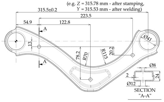
Figure 1.
A research object and the dimension to be examined.

Table 1.
Chemical composition (weight%) and mechanical properties of tested material [36].
Welding of the stampings was carried out using an OTC DM-400 welding machine (OTC Daihen Europe, GmbH., Mönchengladbach, Germany) in combination with an Almega AX V6 welding robot (OTC Daihen Europe, GmbH., Mönchengladbach, Germany) [36]. A number of parameters are related to the welding technology, with current, voltage, and welding speed being important and precisely controllable. In the selected configuration, the device allows for automatic voltage determination. Since this option is used in practice, the voltage parameter was not further investigated with respect to the multicollinearity of the linear model. The individual welding parameters are presented in Table 2.
Table 2.
Welding parameters.
The magnitude of the distortion is directly influenced by the rate of heat input. It is determined by the welding speed and the magnitude of the electric current. By combining these parameters, it is possible to weld a part without significant distortion or, on the contrary, due to the material used and its thickness, it is possible to destroy the part. Attention had to be paid to the practical aspect, i.e., the speeds used should not significantly limit the production capacity. The welding technology used is also a limiting factor since, at higher speeds (corresponding to the selected current), it is not possible to ensure the required product quality. Based on these facts and preliminary experiments, electric current values from 160 to 200 A and welding speeds from 50 to 70 cm·min−1 were determined. The sequence of welds and their locations are shown in Figure 2. The overall deflection of the component before and after welding was measured on a Romer Absolute Arm. The monitored dimension can only be evaluated indirectly since it is determined by the locations of the centres of the two cylindrical holes. A measuring touch was used to record the position of approximately 20 points along the circumference of each cylindrical hole. By using PolyWorks|InspectorTM software, these circles were projected onto the plane of stamping and translated using the measured points. A measurement of the deviation of the resulting shape from the 3D model of the parts [36] was also made during the experiments, but these measurements were not essential for the purposes of this paper.
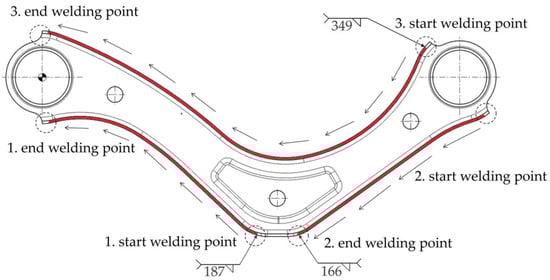
Figure 2.
Location of welds and their order during welding [36].
The experiment was carried out according to Table 3, with individual measurements taken in order according to column nE. The random order of the performed experiments (nE represents the random order) ensures that the assumptions of the methodology of the design of experiment are met, which is necessary for the generalization of the results. Due to the impossibility of taking measurements at the mean value of the stamping dimension (Z), the monitored dimensions of the stampings were chosen at the lower and upper limits of the monitored interval.
Table 3.
Measurements—LR model and training (for ANN) data.
To validate the models, the data (Table 4) from another stamping dimension–316.08 mm were used. These data were not used in the construction of linear regression model (LR) or in learning ANNs.
Table 4.
Measurements—testing data.
2.1. Linear Regression
R, a programming language for statistical computing and graphics, was used in this study. A regression analysis was used to identify relationships between input factors and response factors. The function between the output and output factors can be given in the form:
where Y response (dependent variable), β0 to βn are equation parameters for linear relationship, and X1 to Xn are input factors (independent variables. In our previous paper [36], a prediction model based on linear regression and an experimental methodology using pseudo-central points and face-centred axial points in CCD was presented. This demonstrated the statistical significance of basic process parameters, namely welding current and welding speed in combination with the changing size of the stamping at a significance level of 5%. The predictive power of the model expressed by the adjusted index of determination represents a value of 96.9%. The residual analysis confirmed the validity of the model in the vicinity of the central level of the stamping size factor.
2.2. Artificial Neural Networks
Artificial neural networks are based on the basic structure of the human brain. ANNs consist of a number of simple and highly interconnected processing elements, similar to neurons in the brain. Basically, the model is a black box containing a series of equations used to calculate the outcome based on the inputs [37,38]. Figure 3 illustrates a block diagram of the neuron model.
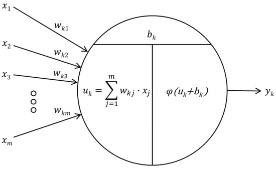
Figure 3.
A nonlinear model of a neuron.
According to the following Equations (2) and (3), a neuron k may be mathematically described as follows [39]:
Neuron inputs are marked as x1, x2,…, xm, and the weights of the individual inputs are marked as wk1, wk2,…, wkm. The output signal from the neuron yk is the result of the activation function φ (.), whose argument determines the sum of the linear combination of inputs and weights uk adjusted by the value of the distortion bk. It is the principle of ANNs to determine the weights and distortions so that the output of the network is as close to the target as possible [40]. A reverse propagation algorithm was used in the learning process of the network based on Levenberg–Marquardt (LM) and Bayesian regularization (BR).
In the hidden layer, the logistic sigmoid nonlinear function for ANN with LM learning algorithm (LMANN) and a hyperbolic tangent function for ANN with Bayesian regularization (BRANN) were used as activation functions. For both networks, the linear transfer function was used as an activation function in the output layer. Due to the mathematical properties of neural networks and activation functions, it is appropriate to normalise the input and output data. Neural networks can also work with non-normalised data, but mostly with lower accuracy and a higher number of neurons. For the LMANN case, the data have been normalised according to the relation (4):
where X is the original input value, Xmin is the minimum input value within the monitored interval, Xmax is the maximum input value within the monitored interval, and Xnorm is the normalised input value for the monitored interval ranging from 0 to 1.
The data for BRANN were also normalized according to the relation (5):
where X is the original input value, Xmin is the minimum input value within the monitored interval, Xmax is the maximum input value within the monitored interval, and Xnorm is the normalised input value for the monitored interval ranging from −1 to 1.
3. Results and Discussion
3.1. LR Results
According to the previous work [36], the following equation has been established for the final dimension of the welded part:
In Figure 4, a comparison of experimental and predicted data is presented.
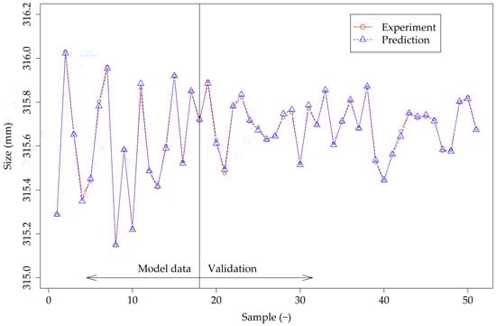
Figure 4.
Comparison between prediction and experimental data for LR.
Figure 5 shows the regression plots for LR. The figure presents a correlation between the experimental and predicted values of the resulting dimension of the welded part for a set of CCD points, for test data gathered near the central level of the input factor of the dimension of the welded part Z and finally for the entire dataset. Figure 5 shows that all the data are close to the 45° line representing R equal to 1, which represents the minimal deviation from the predicted data.
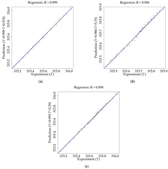
Figure 5.
Regression plots for Linear regression model (LR): (a) training data; (b) testing data; (c) all data.
As shown in Figure 6, the graphical output of the model shows how the resulting dimension of the part is related to the welding speed and current, specifically for the dimension of the stampings Z = 316.00 mm.
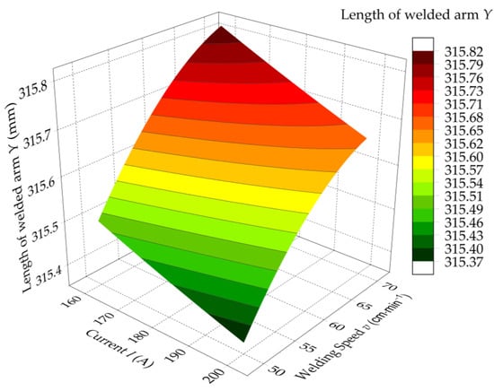
Figure 6.
Dimension of the part as a function of welding speed and current (stampings dimension Z = 316.00 mm).
According to this graph, maximum deformations (smaller resulting dimensions of the welded stamping Y) are achieved at higher currents and lower welding speeds, i.e., while producing more heat. In addition, it is clearly evident from the graph that it is not a general plane, but rather a curved surface as a result of the welding speed (Equation (6)).
3.2. ANN Results
The main structure of ANNs is shown in Figure 7. The structure with a single hidden layer was used.
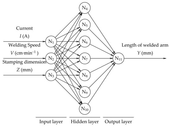
Figure 7.
The main structure of ANN.
The input layer consists of three neurons, and the output layer consists of one neuron. The number of neurons in the hidden layer (seven) was chosen based on preliminary testing of neural networks for the two selected learning algorithm types. Table 5 summarizes the properties of the two ANNs used. The following settings were used to train LMANN: epochs = 1000, mu = 0.001, mu_dec = 0.1 and mu_inc = 10, momentum = 0.9 and LR = 1.2. In order to train the BRANN, the following settings were used: epochs = 1000, mu = 0.005, mu_dec = 0.1, and mu_inc = 10. For each training session, the weights were randomized. As soon as default minimum gradient reached a certain value, all trainings were stopped. In order to compare ANNs and LR, our decision was to train ANNs primarily using DOE data only, which in this case greatly simplifies the comparison of different models.
Table 5.
Properties of the used ANNs.
The LMANN-based prediction equation for the final dimension of the welded part is given by the equation:
Each of the values were calculated using the Logistic Sigmoid function [41]:
Values of exponents were calculated as follows:
The values of weights and biases for LMANN are presented in Table 6.
Table 6.
Weight and bias values between input and hidden layer for LMANN.
Similarly, the BRANN-based prediction equation for the resulting dimension of the welded part is given by the equation:
Each value was calculated using the Hyperbolic Tangent function [41]:
Values of exponents were calculated as follows:
The values of weights and biases for BRANN are presented in Table 7.
Table 7.
Weight and bias values between input and hidden layer for BRANN.
Figure 8 and Figure 9 demonstrate a comparison between the outputs of the individual neural networks and the experimental data for LMANN and BRANN.
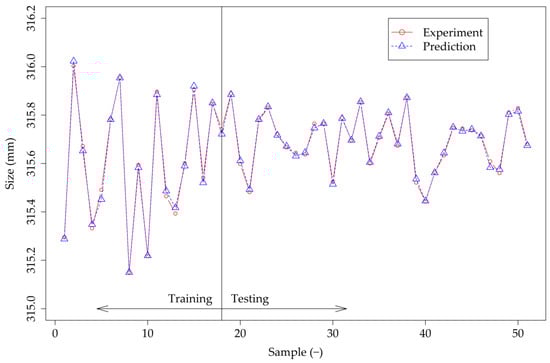
Figure 8.
Comparison between prediction and experimental data for LMANN.
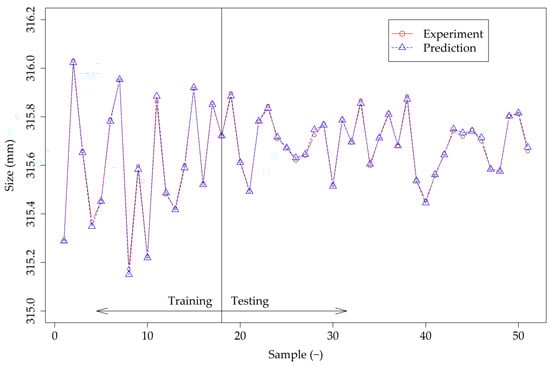
Figure 9.
Comparison between prediction and experiment data for BRANN.
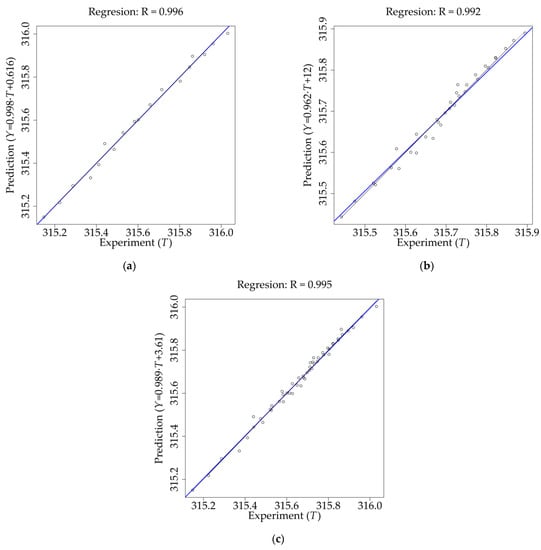
Figure 10.
Regression plots for an artificial neural network with Levenberg–Marquardt back-propagation algorithm (LMANN): (a) training data; (b) testing data; (c) all data.
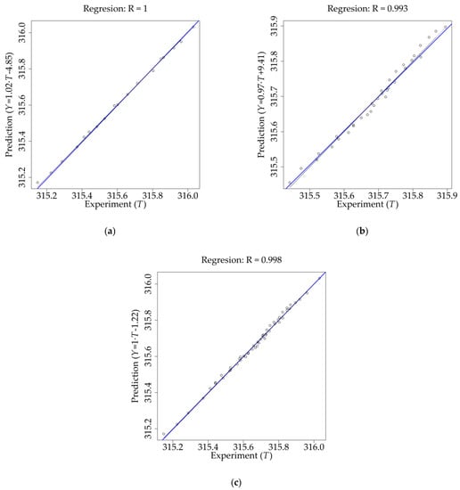
Figure 11.
Regression plots for an artificial neural network with Bayesian regularisation back-propagation algorithm (BRANN): (a) training data; (b) testing data; (c) all data.
3.3. Perfrormance Comparison for the LR Model and ANN Models
The tightness of the model output and target values can be assessed in several ways. Several indicators can be used when comparing linear regression and neural network models. Due to the common practice of providing regression plots when evaluating neural networks, the values of the regression coefficients (R) are summarized in Table 8. The values of root mean square error (RMSE) and mean absolute percentage error (MAPE) are also reported.
Table 8.
Selected performance values of the applied models.
The high accuracy of the regression model is evident from the above data. BRANN also achieves similar accuracy. LMANN lags slightly behind, but this model can also be assessed as highly accurate. When evaluating the performance of the models, it should be noted that training ANNs on such a low number of data is not common. However, the main advantage of the experimental methodology is the high accuracy of the model with a reduced number of measurements, and the results of ANNs show that neural networks can be successfully used in this field as well. It can be expected that repeated training of ANNs using additional measurements will result in a model that is more accurate than the original LR model. Figure 12 illustrates the potential of this approach by showing the MAPE values for all data, while the neural networks were gradually trained on a larger number of data sets.
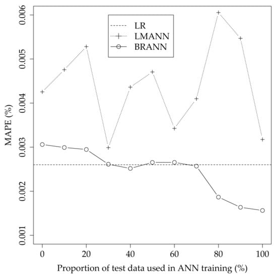
Figure 12.
The dependence of MAPE (all data) on the used set of training data.
4. Conclusions
This paper deals with the implementation of neural networks in the process of welding stampings in the automotive industry and increasing the accuracy of the final dimension of the component under study. The well-known dependence of product dimension on many factors is often a limiting factor for this combination of technologies. It has been confirmed that the resulting dimension can be corrected by exploiting the thermal distortion during welding, while neural networks can also be used to determine the optimal welding parameters.
There are two models presented in this paper, namely a Levenberg–Marquardt back-propagation algorithm and a Bayesian regularised back-propagation algorithm, which are used as the learning algorithms for neural networks in multi-layer feed-forward networks. Based on the design of experiments methodology, the models have been compared to a mathematical model with similar accuracy.
The results can be summarised as follows:
- Neural networks can be trained on reduced number of samples of data based on a design of experiment methodology.
- The new derived Equations (7) and (10) can be used to predict the resulting dimension directly from the input operating parameters within the considered interval.
- It was observed that linear regression had the lowest MAPE when training the ANN using DOE data. Despite the low number of training data, the neural network with Bayesian regularized back propagation algorithm achieved comparable results.
- MAPE for ANN with Levenberg–Marquardt back-propagation algorithm fluctuated around a value of 4 × 10⁻³%, which is greater than that for LR.
- MAPE for ANN with Bayesian regularized back-propagation algorithm trained on DOE data was at the MAPE level of 3 × 10⁻³%. However, the accuracy of the model increased with the increase of the training dataset up to the level of 1.6 × 10⁻³%.
Author Contributions
Conceptualisation, M.K. (Milan Kadnár) and P.K.; methodology, M.K. (Milan Kadnár), M.H. and J.V.; validation, M.B. (Marián Bujna) and R.M.; formal analysis, M.B. (Marián Bujna) and M.B. (Marian Boržan); investigation, P.K. and F.T.; data curation, M.B. (Marián Bujna) and M.K. (Milena Kušnerová); writing-original draft preparation, M.H.; writing-review and editing, J.V.; visualization, F.T. and R.M.; project administration, M.H.; funding acquisition, R.M. All authors have read and agreed to the published version of the manuscript.
Funding
This research work has been supported by Ministry of Education, Science, Research and Sport of the Slovak Republic by the grant VEGA: 1/0236/21.
Institutional Review Board Statement
Not applicable.
Informed Consent Statement
Not applicable.
Data Availability Statement
The data presented in this study are available on request from the corresponding author after obtaining permission of authorized person.
Conflicts of Interest
The authors declare no conflict of interest.
References
- Ozcelik, S.; Moore, K. Modeling, Sensing and Control of Gas Metal Arc Welding; Elsevier: Amsterdam, The Netherlands, 2003. [Google Scholar]
- Cary, H.B. Arc Welding Automation; Marcel Dekker: New York, NY, USA, 1995. [Google Scholar]
- Omar, M.A. The Automotive Body Manufacturing Systems and Processes; John Wiley & Sons: Hoboken, NJ, USA, 2011. [Google Scholar]
- Zong, R.; Chen, J.; Wu, C. A comparison of TIG-MIG hybrid welding with conventional MIG welding in the behaviors of arc, droplet and weld pool. J. Mater. Process. Technol. 2019, 270, 345–355. [Google Scholar] [CrossRef]
- Noga, P.; Tuz, L.; Żaba, K.; Zwoliński, A. Analysis of Microstructure and Mechanical Properties of AlSi11 after Chip Recycling, Co-Extrusion, and Arc Welding. Materials 2021, 14, 3124. [Google Scholar] [CrossRef] [PubMed]
- Tuz, L.; Kąc, S.; Sierakowski, D. Technology of electron beam welding of 10CrMo9-10 steel with the specific quality requirements. Manuf. Lett. 2023, 35, 53–57. [Google Scholar] [CrossRef]
- Weman, K.; Gunnar, L. MIG Welding Guide; Woodhead Publishing: Cambridge, England, 2006. [Google Scholar]
- Sun, Z.; Yu, X. Prediction of welding residual stress and distortion in multi-layer butt-welded 22SiMn2TiB steel with LTT filling metal. J. Mater. Res. Technol. 2022, 18, 3564–3580. [Google Scholar] [CrossRef]
- Liang, W.; Murakawa, H. Predicting welding distortion in a panel structure with longitudinal stiffeners using inherent deformations obtained by inverse analysis method. Sci. World J. 2014, 2014, 601417. [Google Scholar] [CrossRef]
- Heinze, C.; Schwenk, C.; Rethmeier, M. The effect of tack welding on numerically calculated welding-induced distortion. J. Mater. Process. Technol. 2012, 212, 308–314. [Google Scholar] [CrossRef]
- Luo, M.; Hu, R.; Li, Q.; Huang, A.; Pang, S. Physical understanding of keyhole and weld pool dynamics in laser welding under different water pressures. Int. J. Heat Mass Transf. 2019, 137, 328–336. [Google Scholar] [CrossRef]
- Guu, A.; Rokhlin, S. Arc weld process control using radiographic sensing. Mater. Eval. 1992, 50, 1344–1348. [Google Scholar]
- Han, Y.; Fan, J.; Yang, X. A structured light vision sensor for on-line weld bead measurement and weld quality inspection. Int. J. Adv. Manuf. Tech. 2019, 106, 2065–2078. [Google Scholar] [CrossRef]
- Huang, N.; Zhang, J.; Zhang, T.; Zheng, X.; Yan, Z. Control of Welding Speed and Current in Machine–Human Cooperative Welding Processes. Crystals 2022, 12, 235. [Google Scholar] [CrossRef]
- Liu, Y.; Zhang, W.; Zhang, Y. Dynamic Neuro-Fuzzy-Based Human Intelligence Modeling and Control in GTAW. IEEE Trans. Autom. Sci. Eng. 2015, 12, 324–335. [Google Scholar] [CrossRef]
- Chandrasekhar, N.; Vasudevan, M.; Bhaduri, A.K.; Jayakumar, T. Intelligent modeling for estimating weld bead width and depth of penetration from infra-red thermal images of the weld pool. J. Intell. Manuf. 2013, 26, 59–71. [Google Scholar] [CrossRef]
- Guzmán, L.G.; Hammett, P.C. A Tolerance Adjustment Process for Dimensional Validation of Stamping Parts and Welded Assemblies; International Body Engineering Conference & Exposition; Society of Automotive Engineers (SAE): Warrendale, PA, USA, 2003. [Google Scholar]
- Lee, D.; Kwon, K.E.; Lee, J.; Jee, H.; Yim, H.; Cho, S.W.; Shin, J.-G.; Lee, G. Tolerance Analysis Considering Weld Distortion by Use of Pregenerated Database. J. Manuf. Sci. Eng. 2009, 131. [Google Scholar] [CrossRef]
- Michaleris, P.; DeBiccari, A. Prediction of welding distortion. Weld. J. Includ. Weld. Res. Suppl. 1997, 76, 172s. [Google Scholar]
- Reisgen, U.; Sharma, R.; Christ, M.; Mann, S. Method development of statistical modeling for the description of welding fume emissions in gas metal arc welding using transient process characteristics. Weld. World 2020, 64, 1497–1502. [Google Scholar] [CrossRef]
- Mallieswaran, K.; Padmanabhan, R.; Balasubramanian, V. Friction stir welding parameters optimization for tailored welded blank sheets of AA1100 with AA6061 dissimilar alloy using response surface methodology. Adv. Mater. Process. Technol. 2018, 4, 142–157. [Google Scholar] [CrossRef]
- Artinov, A.; Karkhin, V.; Bachmann, M.; Rethmeier, M. Mathematical modeling of the geometrical differences between the weld end crater and the steady-state weld pool. J. Laser Appl. 2020, 32, 022024. [Google Scholar] [CrossRef]
- Daunys, M.; Dundulis, R.; Kilikevičius, S.; Česnavičius, R. Analytical investigation and numerical simulation of the stress–strain state in mechanically heterogeneous welded joints with a single-V butt weld. Eng. Fail. Anal. 2016, 62, 232–241. [Google Scholar] [CrossRef]
- Nasiri, M.B.; Enzinger, N. An analytical solution for temperature distribution in fillet arc welding based on an adaptive function. Weld. World 2018, 63, 409–419. [Google Scholar] [CrossRef]
- Reisgen, U.; Schleser, M.; Mokrov, O.; Ahmed, E. Optimization of laser welding of DP/TRIP steel sheets using statistical approach. Opt. Laser Technol. 2012, 44, 255–262. [Google Scholar] [CrossRef]
- Mikno, Z.; Grzesik, B.; Stępień, M. The investigation on the ideal spot weld numerical model in resistance welding. Int. J. Adv. Manuf. Tech. 2020, 111, 895–907. [Google Scholar] [CrossRef]
- Mohanty, U.K.; Sharma, A.; Abe, Y.; Fujimoto, T.; Nakatani, M.; Kitagawa, A.; Tanaka, M.; Suga, T. Thermal modelling of alternating current square waveform arc welding. Case Stud. Therm. Eng. 2021, 25, 100885. [Google Scholar] [CrossRef]
- Abdelhafeez Hassan, A.; Küçüktürk, G.; Yazgin, H.V.; Gürün, H.; Kaya, D. Selection of Constitutive Material Model for the Finite Element Simulation of Pressure-Assisted Single-Point Incremental Forming. Machines 2022, 10, 941. [Google Scholar] [CrossRef]
- Kim, J.-J.; Bae, M.; Hong, M.-P.; Kim, Y.-S. Finite Element Analysis on Welding-Induced Distortion of Automotive Rear Chassis Component. Metals 2022, 12, 287. [Google Scholar] [CrossRef]
- Amirsalari, B.; Golabi, S.I. Finite element analysis, prediction, and optimization of residual stresses in multi-pass arc welding with experimental evaluation. J. Strain. Anal. Eng. Des. 2022, 57, 305–320. [Google Scholar] [CrossRef]
- Ma, B.; Meng, D.; Gu, X.; Ma, X.; Zhang, D.; Zhang, Q. Integration process of stamping and welding for DP600 advanced high strength steel sheets. Procedia Manuf. 2018, 15, 684–692. [Google Scholar] [CrossRef]
- Kang, W.; Cheon, S.S. Analysis of coupled residual stresses in stamping and welding processes by finite element methods. Proc. Inst. Mech. Eng. B J. Eng. Manuf. 2012, 226, 884–897. [Google Scholar] [CrossRef]
- Fentaye, A.D.; Zaccaria, V.; Kyprianidis, K. Aircraft Engine Performance Monitoring and Diagnostics Based on Deep Convolutional Neural Networks. Machines 2021, 9, 337. [Google Scholar] [CrossRef]
- Fahle, S.; Prinz, C.; Kuhlenkötter, B. Systematic review on machine learning (ML) methods for manufacturing processes—Identifying artificial intelligence (AI) methods for field application. Procedia CIRP 2020, 93, 413–418. [Google Scholar] [CrossRef]
- Hamedi, M.; Shariatpanahi, M.; Mansourzadeh, A. Optimizing spot welding parameters in a sheet metal assembly by neural networks and genetic algorithm. Proc. Inst. Mech. Eng. B J. Eng. Manuf. 2007, 221, 1175–1184. [Google Scholar] [CrossRef]
- Kadnár, M.; Káčer, P.; Harničárová, M.; Valíček, J.; Gombár, M.; Kušnerová, M.; Tóth, F.; Boržan, M.; Rusnák, J. Prediction Model of the Resulting Dimensions of Welded Stamped Parts. Materials 2021, 14, 3062. [Google Scholar] [CrossRef]
- Kalogirou, S.A. Artificial neural networks in renewable energy systems applications: A review. Renew. Sustain. Energy Rev. 2001, 5, 373–401. [Google Scholar] [CrossRef]
- Ozgoren, M.; Bilgili, M.; Sahin, B. Estimation of global solar radiation using ANN over Turkey. Expert Syst. Appl. 2012, 39, 5043–5051. [Google Scholar] [CrossRef]
- Haykin, S. Neural Networks: A Comprehensive Foundation; Prentice Hall PTR: Upper Saddle River, NJ, USA, 1999. [Google Scholar]
- Bilgili, M.; Sahin, B. Comparative analysis of regression and artificial neural network models for wind speed prediction. Meteorol. Atmos. Phys. 2010, 109, 61–72. [Google Scholar] [CrossRef]
- Nele, L.; Mattera, G.; Vozza, M. Deep Neural Networks for Defects Detection in Gas Metal Arc Welding. Appl. Sci. 2022, 12, 3615. [Google Scholar] [CrossRef]


Disclaimer/Publisher’s Note: The statements, opinions and data contained in all publications are solely those of the individual author(s) and contributor(s) and not of MDPI and/or the editor(s). MDPI and/or the editor(s) disclaim responsibility for any injury to people or property resulting from any ideas, methods, instructions or products referred to in the content. |
© 2023 by the authors. Licensee MDPI, Basel, Switzerland. This article is an open access article distributed under the terms and conditions of the Creative Commons Attribution (CC BY) license (https://creativecommons.org/licenses/by/4.0/).