Abstract
This paper deals with the stabilization problem of a nonlinear system described by a Takagi–Sugeno fuzzy (TSF) model with unmeasurable premise variables via a robust controller. Applying the sector nonlinearity techniques, the nonlinear system is represented by a decoupled fuzzy model. Then, we design a robust observer-based controller for the obtained fuzzy system by utilizing the differential mean value approach. The observer and controller gains are obtained by the separation principle, in which the problem is solved in the sum of linear matrix inequalities (LMIs). The paper presents two main contributions: A state feedback controller is designed using differential mean value (DMVT) which ensures robust stabilization of the nonlinear system. Additionally, the Luenberger observer is extended to the Takagi–Sugeno fuzzy models. The second contribution is to reduce conservatism in the obtained conditions, a non-quadratic Lyapunov function (known as the line integral Lyapunov fuzzy candidate (LILF)) is employed. Two examples are provided to further illustrate the efficiency and robustness of the proposed approach; specifically, the Takagi–Sugeno fuzzy descriptor of an induction motor is derived and a robust observer-based controller applied to the original nonlinear system.
1. Introduction
Induction motors, also known as asynchronous motors, are widely used in industrial applications because of their numerous advantages. They are simple in design, robust in operation and relatively inexpensive to purchase and maintain. Additionally, they can be found in a wide range of sizes and power ratings, making them suitable for a variety of industrial applications [1]. Unfortunately, these machines are nonlinear systems that can be difficult to control due to variations in parameters and the inaccessibility of the rotor flux. This makes controlling the speed and torque of an induction motor challenging compared to other types of motors.
Physical systems are often represented by nonlinear models because they are better able to accurately describe the complex behavior of the system. Nonlinear models can capture the full range of possible behaviors, which can lead to better reliability and performance when simulating or predicting the behavior of the system. However, as this model becomes more detailed and accurate, it often becomes more complex and harder to analyze [2,3].
The Takagi–Sugeno fuzzy system is a powerful mathematical model used to represent nonlinear systems. It is based on fuzzy logic and has been shown to accurately represent nonlinear systems without losing any information. This makes it a popular choice for various applications, including the application of theorems originally developed for linear systems [4]. In this approach, the original nonlinear system is decomposed into a set of linear sub-systems and each sub-system is associated with a nonlinear membership function (MF) that describes the degree to which it belongs to a particular set. The membership functions are typically defined as fuzzy sets and are used to partition the state space of the system into a finite number of regions. Each region is associated with a linear sub-system and the output of the overall system is a weighted combination of the outputs of each sub-system. This approach allows for more accurate and flexible control of the system as it can account for variations and uncertainties in the system’s behavior. The use of fuzzy logic and membership functions provides a natural way to handle uncertainties and nonlinearities in the system. Takagi–Sugeno models are often achieved by using the sector nonlinearity transformation, which transforms the nonlinear system into a set of linear sub-systems with nonlinear inputs [5].
Quadratic Lyapunov functions can be used to determine the stability analysis and design an observer or controller for the fuzzy system whose constraints are written as linear matrix inequalities, these conditions can be effectively solved by convex programming techniques [6,7]. Finding a common positive definite matrix that satisfies all constraints derived by the quadratic Lyapunov function can be a difficult task and may lead to a conservative solution. Additionally, finding such a matrix may require a significant amount of computation, which can further add to the complexity of the problem [8]. Conservatism in T-S fuzzy systems can be attributed to several factors, including the approach and type of T-S fuzzy system used [9], the method used to obtain linear matrix inequality constraints from the membership functions [10] and the choice of the Lyapunov function used in the stability analysis [11]. Each of these factors can introduce additional conservatism into the system, potentially leading to a less robust or less accurate control system. Polyquadratic fuzzy Lyapunov functions (PFLFs) [12,13], line integral functions (LIFs) [14,15] and piecewise Lyapunov functions (PWLFs) [16,17] are two techniques that have been developed to reduce this conservatism. These approaches can help to relax the constraints and improve the performance of the controller. Unfortunately, due to the overlap of the membership functions, the piecewise Lyapunov functions are inadequate for Takagi–Sugeno fuzzy models derived from sector nonlinearity techniques [18]. Moreover, the constraints derived from the controller synthesis using these functions are expressed in the form of bilinear matrix inequalities, which can pose challenges for solving optimization problems. In such cases, it may be necessary to explore alternative methods, such as using multiple Lyapunov functions. This approach entails determining matrices for each sub-system of the fuzzy system and creating a candidate function by using the obtained matrices [19]. However, the use of derivatives of membership functions in controller design can make the problem more complex because it requires the evaluation of upper bounds on the derivatives. The line integral Lyapunov function is defined as the integral of a scalar function along a trajectory of the system, which must be positive definite along this trajectory [16,20]. It can be noted that the function studied in this paper can be regarded as a particular form of the conventional quadratic function, where the stability conditions associated with these functions are less stringent than those of the quadratic Lyapunov function.
Motivated by [20,21], a new method for stabilizing a nonlinear system represented by a Takagi–Sugeno fuzzy system with external perturbation and unmeasurable premise variables is given based on the control and mean value theorem.
The manuscript presents several key contributions: Firstly, the use of a line integral Lyapunov function offers a less strict condition for control design, particularly when the time derivative of membership functions is not available. This allows for greater flexibility in control system design and can lead to improved performance and stability. Secondly, the proposed control system utilizes the mean value theorem method to obtain observer and controller gains through linear matrix inequalities. This approach offers a systematic and efficient method for controller design. Finally, the manuscript presents a novel observer-based robust state feedback control system for a three-phase induction motor represented with a Takagi–Sugeno fuzzy system. This control system offers improved performance and robustness over existing control systems.
The other parts of this work are organized as follows: The problem statement and backgrounds are presented in Section 2. In Section 3, we use the mean value theorem and a non-quadratic function to design a state feedback controller for the T-S fuzzy systems. Section 4 presents the validation of the suggested approach via a numerical example. Additionally, in order to demonstrate the efficiency of the controller, an application to an induction motor is discussed. Finally, some conclusions are given.
2. Problem Statement and Backgrounds
Consider a nonlinear dynamical system, which is given by:
where f and g are smooth nonlinear matrices functions and are the states; is the control input vector; is the measurement vector; all variables are assumed to be bounded on a compact set .
The Takagi–Sugeno fuzzy system uses a set of fuzzy if–then rules to make predictions or control decisions based on input data and the linear model component allows for precise modeling of complex systems.
Consider the following T-S fuzzy system structure:
Rule
IF is , …and is
THEN
where are fuzzy sets; is the state; l denotes the number of fuzzy rules and p denotes the number of premise variables.
is the vector of premise variables
and are real constant matrices of adequate dimensions.
r is the local sub-model number.
2.1. Differential Mean Value Theorem
The controller gains will be derived using the mean value theorem approach, which will be presented in this subsection.
Theorem 1
([22]). Let : be a function continuous in and differentiable in the convex hull of the set . For , there exist and for , such that:
2.2. Non-Quadratic Lyapunov Function Candidate
In this subsection, we consider the so-called line integral fuzzy Lyapunov function. Rhee et al. [21] developed the following function:
where the term represents the path in the domain that starts at the origin (zero) and ends at x. represents a dummy vector for the integral and an infinitesimal displacement vector, respectively. However, can be represented by a force vector at x; the suggested Lyapunov function candidate in (6) can be considered as the work officiated in from the origin zero to x. The candidate must meet the following requirements: (1) is a continuously differentiable function, (2) positive definite and (3) radially unbounded. However, the condition (2) and (3) cannot be satisfied if the function is dependent on the is independent of the path if
and
where
3. Main Results
3.1. Stability Analysis
3.1.1. Analysis Based on Quadratic Function
Typically, the Lyapunov direct approach is employed to achieve stability analysis and stabilization for Takagi–Sugeno fuzzy models derived from linear or bilinear matrix inequality conditions. In this section, we present simple criteria for verifying the stability of a Takagi–Sugeno fuzzy model employing a quadratic Lyapunov function.
Consider the Takagi–Sugeno fuzzy system defined as follows:
Theorem 2
([4]). System (9) is globally asymptotically stable if there exists such that the next linear matrix inequalities hold
3.1.2. Analysis Based on Non-Quadratic Function
The following theorem gives the conditions sufficient to assure the asymptotic stability of an autonomous fuzzy model applying LIFF.
Theorem 3.
Proof of Theorem 3 in Appendix A.
3.1.3. With Non Quadratic Functions
The controller is designed using the classical state feedback
Theorem 4.
By utilizing the H performance extension (Appendix B), the 29 linear matrix inequalities are transformed to the following:
where
3.2. Observer-Based State Feedback Controller
This section describes the design of a robust observer-based controller for the global T-S fuzzy system where external disturbances are added. Consider the following: T-S fuzzy model with external disturbances and for the case without uncertainties.
where denotes the unknown input vector.
Thus, the description of the corresponding state fuzzy observer is as follows:
where is the estimated system state; is the estimated premise vector which depends on the estimated state variables; L is the observer gain matrix. Using the estimated state, the following control law is used to design an observer-based states classical feedback controller for robust stabilization of system (24):
where K is the fuzzy controller gain with appropriate dimensions.
4. Numerical Examples
In this section, the effectiveness of the proposed strategy is demonstrated through two numerical examples.
Example 1.
Let us consider the following nonlinear model.
The T-S fuzzy model is given as the following form:
where the matrices are given as follows:
The range of values ( and ) is used to compare the feasible regions of the LMI-based problems discussed in Theorems 2 and 3.
Figure 1 illustrates the comparison between the stability region derived from the linear matrix inequalities of the classical Lyapunov function in Theorem 1 and the non-quadratic conditions outlined in Theorem 2. As expected, it is clear that the proposed non-quadratic functions produce less restrictive results compared to the traditional quadratic functions. This demonstrates the enhancement in the level of conservativeness for the stabilization problem using non-quadratic functions that is presented in this work.
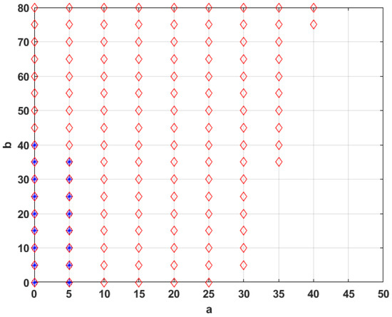
Figure 1.
Comparison of the feasibility fields on parameter space obtained via Theorems 2 “*” and 3 “⋄”.
Remark 1.
If the values of the parameters a and b are set to and 10, respectively, the stabilization criteria given by Theorem 2 cannot be satisfied. This implies that it is not possible to obtain a stable controller using these methods. However, by utilizing Theorem 3, the stabilization conditions can be resolved within linear matrix inequality regions.
For the specific point where and , only one solution was obtained using Theorem 3. This solution is represented by the state-feedback control law given in Equation (14) and the gain matrices are determined under linear matrix inequality constraints. By applying Theorem 1 to this model, a feasible solution is obtained with the following robust extended controller and observer gains.
With quadratic case:
the positive definite matrices can be obtained as:
With non-quadratic function:
the positive definite matrices can be obtained as:
We note that the initial conditions are and . The simulation results of the closed-loop state trajectories can be seen in Figure 2. Moreover, we considered the perturbation dynamics given in (20) with .
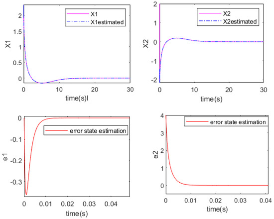
Figure 2.
State evolution of T-S fuzzy model under control law obtained via Theorem 4.
Figure 3 indicates that it is possible to achieve system stability by setting higher values for the observer and controller gains. Furthermore, the method presented in this study offers a practical solution for determining the optimal H-attenuation level.
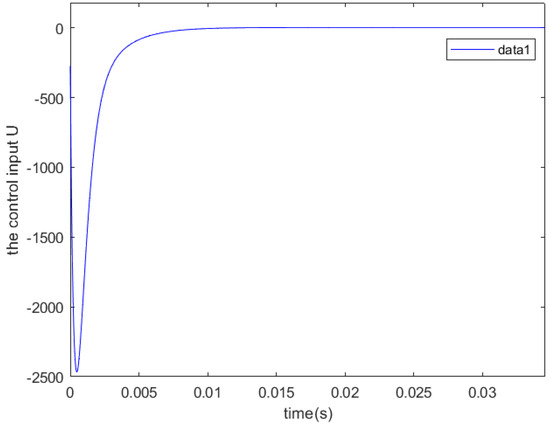
Figure 3.
Control law evolution with gains obtained via Theorem 4.
Example 2.
Induction Motor
Electrical Dynamic Model of IM
In this subsection, we will describe the behavior of the induction machine. To make the presentation more manageable, we will use certain simplifying assumptions. By applying Park’s transformation to the system of equations, we can derive a two-phase model in the d-q frame. This model is based on the idea of transforming the three-phase quantities into a two-dimensional, orthogonal frame of reference. In this frame, the two axes represent the direct and quadrature components of the three-phase quantities, respectively. The resulting two-phase model is widely used in the analysis and control of such machines.
The state space model of the induction motor is represented in the d-q reference frame using several variables. These variables include the stator current components (), the rotor flux components (), the electrical speed of the stator () and the stator voltage components (usd, usq). In this model, the state variables are the stator current components and the rotor flux components. The input variables are the stator voltage components and the disturbance variables are the electrical speed of the stator or any other external disturbances. In the d-q frame, the equations can be simplified and written in matrix form, where the state variables and input variables are represented as matrices. The resulting state space model provides a useful representation of the dynamic behavior of the induction motor, which can be analyzed and controlled using several techniques.
The mathematical representation of the induction motor in the synchronous d-q reference frame is presented as follows [23].
where
where , , , , ; and are the state, control and output vectors, respectively.
The characteristics of the motor can be described using several parameters, including the stator resistance (Rs), stator inductance (Ls), rotor resistance (Rr), rotor inductance (Lr), moment of inertia, mutual inductance (M), friction coefficient (f) and the number of pole pairs (p). These parameters play a crucial role in determining the performance of the motor and are used to derive the mathematical equations that govern the motor’s dynamic behavior.
The reference signal is produced by applying the Field-Oriented Control theorem.
As a result, the control inputs are provided as follows:
with
The decision variables are selected as follows:
Thus the nonlinear terms can be converted into the following form:
where
So the global TS fuzzy system of the induction motors model is established as follows:
Figure 4 displays the schematic diagram of an observer-based state feedback control system that was derived using a non-quadratic function and the mean value theorem. The machine studies is a (7.5 kW) induction motor whose parameters are presented in Table A1 (see Appendix C)
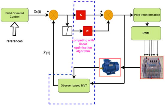
Figure 4.
Observer-based state feedback control structure.
By applying Theorem 4 and using the linear matrix inequality technique, the controller and observer gain matrices of the fuzzy control law (14) can be calculated. The result obtained is as follows:
5. Simulation Results
To emphasize the effectiveness of the proposed approach, a comparative analysis was conducted. Figure 5, Figure 6 and Figure 7 illustrate the motor speed, direct and quadrature axis stator current of an induction motor controlled using two different methods under load torque charging. It can be observed that the rotor speed transient responses with an IP controller display higher peaks compared to the proposed approach when load torque is applied.
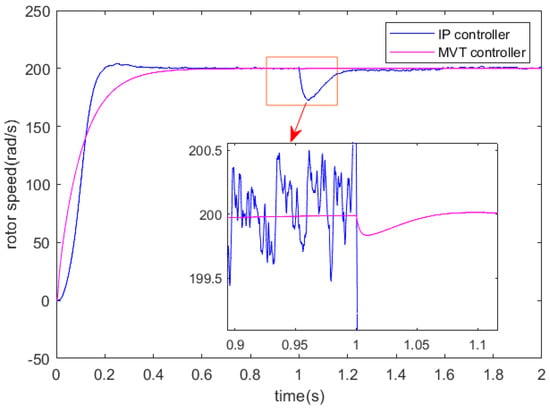
Figure 5.
Rotor speed responses under two controllers.
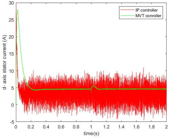
Figure 6.
d-axis current waveform under two controllers.
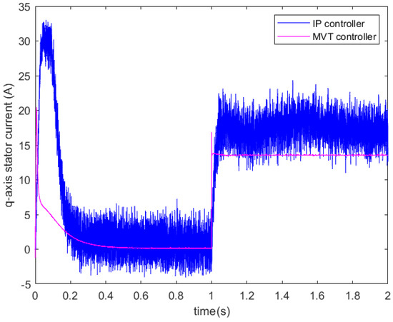
Figure 7.
q-axis current waveform under two controllers.
Table 1 displays a comparison between the rotor speed response indices controlled using the classical approach (IP controller) and the observer-based robust state feedback. It is evident that the proposed technique offers superior performance in comparison to the IP controller. This makes the robust controller a more advantageous option for industrial applications.

Table 1.
Controllers Indexes.
Figure 8 and Figure 9 depict the simulated regulation for the rotor speed and the three phase stator currents, respectively, considering parametric uncertainties in rotor resistance with Rr = 2 Rrn and load torque charging of 20 N·m at t = 1 s. Similarly, Figure 10 and Figure 11 display the results for the motor response under the uncertainties of the moment of inertia (J = 1.5 Jn). These results demonstrate that the proposed control method, utilizing the mean value theorem and the line integral Lyapunov function, is robust and insensitive against variations in Rr and J.
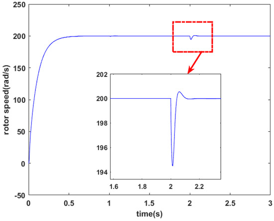
Figure 8.
Rotor speed under variation of Rr.
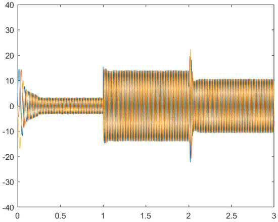
Figure 9.
Stator currents under variation of Rr.
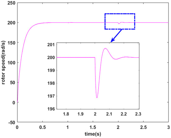
Figure 10.
Rotor speed under variation of J.
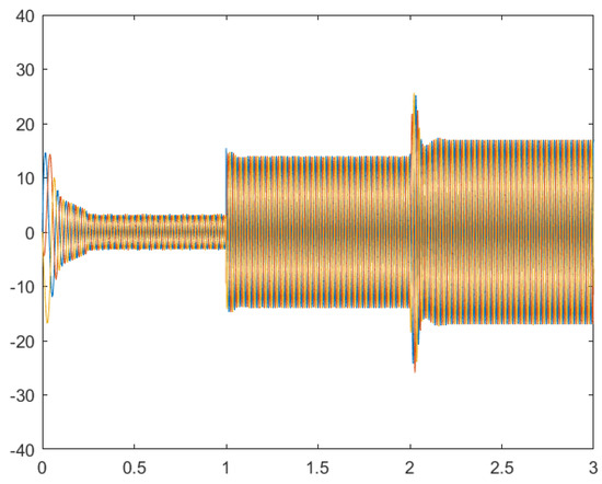
Figure 11.
Stator currents under variation of J.
6. Experimental Results
An experimental evaluation using Real-Time Hardware-in-the-Loop (RT-HIL) simulation of the control method discussed in this paper was conducted and a series of measurements were taken. The experimental setup was developed in the Energy Systems Modeling Laboratory. The hardware structure of the control system was composed of two interconnected dSPACE 1104. The first module reads the feedback currents and the rotor speed and generates the necessary switching signals to operate the induction motor. However, the motor is emulated by the second dSPACE as shown in Figure 12.
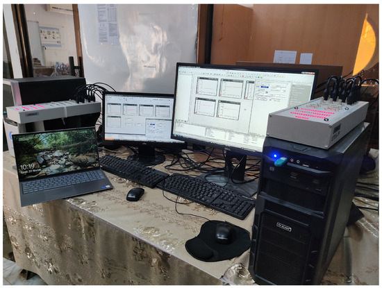
Figure 12.
Test bench.
Figure 13, Figure 14, Figure 15 and Figure 16, respectively, depict the motor speed response, q-axis stator current and d-q axis rotor flux after a step change in speed reference from 200 to 300 rad/s and changing the torque reference from 0 to 20 N·m at s. Figure 13 clearly shows that the rotor speed closely tracks its reference with a fast-settling time and without any noticeable overshoot, during both the increase and decrease stages. Except for the rotor fluxes depicted in Figure 16, the proposed controller demonstrates a negligible tracking error. Figure 15 reveals that the quadrature component of the stator current is directly proportional to variations in load torque. These results indicate and confirm the effectiveness of the proposed control law.
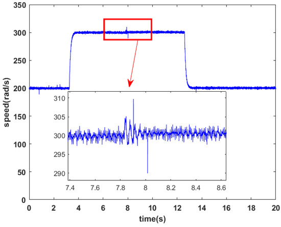
Figure 13.
Rotor speed.
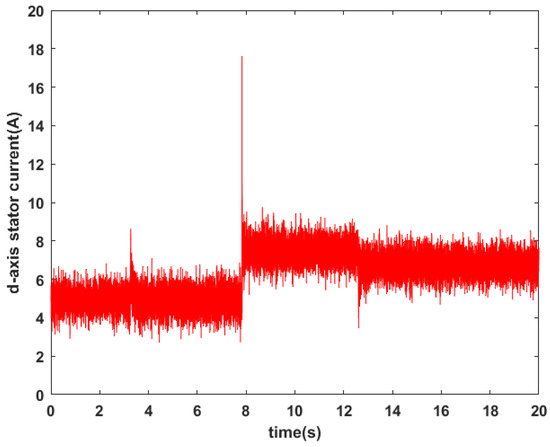
Figure 14.
d-axis stator current.
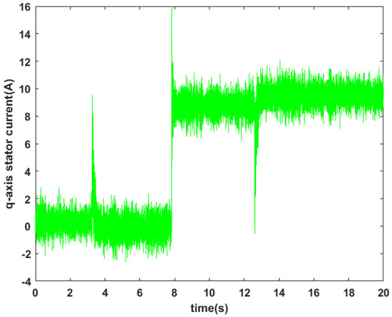
Figure 15.
q-axis stator current.
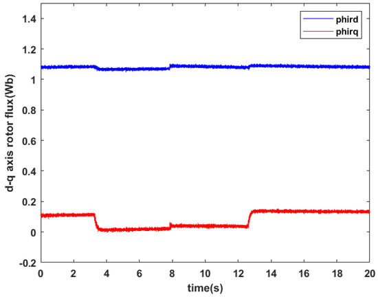
Figure 16.
d-q axis rotor flux.
7. Conclusions
In this paper, an observer-based state feedback controller for a continuous TS fuzzy system with unmeasurable premise variables is proposed. The use of a modified mean value theorem in conjunction with a non-quadratic Lyapunov function can provide new and more general conditions for the stability and stabilization of the TS fuzzy system. The results of the comparison show that the derived stability conditions for the non-quadratic function are more extensive and less conservative than those for the quadratic Lyapunov function. This means that the non-quadratic function is able to provide a wider range of stable solutions and is less restrictive in its conditions for stability compared to the classical, commonly used method. Finally, a numerical example was given to show the effectiveness of the proposed approach. In addition, the results of the real-time implementation have demonstrated that the control system is capable of achieving good tracking and disturbance rejection performance.
In future works, there are several areas that should be considered for further development and improvement of the proposed control system. Firstly, other forms of non-quadratic Lyapunov functions, such as the poly-quadratic function, should be investigated. These alternative Lyapunov functions may offer improved performance or stability properties over the existing quadratic Lyapunov function used in the several control system. Secondly, a fault-tolerant control system should be designed for nonlinear systems described with a Takagi–Sugeno fuzzy model. Finally, a fault detection procedure based on the residuals technique generated from the mean value theorem observer should be developed.
Author Contributions
Conceptualization, R.H. and M.Y.H.; methodology, R.H., M.Y.H., M.B. and A.T.; software, R.H.; validation, R.H., M.Y.H., M.B. and A.T.; formal analysis, R.H., M.Y.H., M.B., and A.T.; investigation, R.H. and M.Y.H.; data curation, R.H. and M.Y.H.; writing-original draft preparation, R.H.; writing-review and editing, R.H., M.Y.H., M.B. and A.T. All authors have read and agreed to the published version of the manuscript.
Funding
This research received no external funding.
Data Availability Statement
Not applicable.
Conflicts of Interest
The authors declare no conflict of interest.
Appendix A. Proof of Theorem 3
Appendix B. Extension for H∞ Performance
The existence of the disturbances will have a effect on control performance. In order to minimize the effects of the disturbance , the H performances associated with the state feedback control error have been considered in [23]
where is the specified disturbance attenuation level.
In order to accomplish linear matrix inequalities constraints, we denotes the error dynamics can be described as
In most situations, Lyapunov’s direct approach is used to obtain the results of stability analysis and stabilization for Takagi–Sugeno fuzzy models which have been derived from linear matrix inequalities or Bilinear matrix inequalities conditions.
where
Therefore, in order to develop the asymptotic stability of (A2) and the state control error’s H∞ performance, we define that:
then
If we consider that we obtain the final linear matrix inequalities to solving:
The controller gain is
Appendix C. Induction Motor Parameters
Table A1 presents the implemented induction motor’s parameters.

Table A1.
Induction motor parameters.
Table A1.
Induction motor parameters.
| Mutual Inductance | H |
| Moment of inertia | Kg·m2 |
| Stator resistance | |
| Rotor resistance | |
| Stator inductance | H |
| Rotor inductance | H |
| Friction coefficient | Nms |
The decision variables are bounded as:
The sets of matrices can be obtained as follows:
and
References
- Alshbib, M.M.; Elgbaily, M.M.; Alsofyani, I.M.; Anayi, F. Performance enhancement of direct torque and rotor flux control (dtrfc) of a three-phase induction motor over the entire speed range: Experimental validation. Machines 2023, 11, 22. [Google Scholar] [CrossRef]
- Boukhlouf, A.; Hammoudi, M.Y.; Saadi, R.; Benbouzid, M.E.H. Hardware-in-the-loop implementation of an unknown input observer for synchronous reluctance motor. ISA Trans. 2023, 133, 485–494. [Google Scholar] [CrossRef]
- Lazarini, A.Z.; Teixeira, M.C.; Jean, M.D.S.; Assunção, E.; Cardim, R.; Buzetti, A.S. Relaxed Stabilization Conditions for TS Fuzzy Systems with Optimal Upper Bounds for the Time Derivative of Fuzzy Lyapunov Functions. IEEE Access 2021, 9, 64945–64957. [Google Scholar] [CrossRef]
- Wang, Z.; Zhao, Y.; Du, H.; Cao, K. Stability analysis of T–S fuzzy control systems subject to actuator saturation. Int. J. Fuzzy Syst. 2019, 21, 2625–2631. [Google Scholar] [CrossRef]
- Pal, D.; Chatterjee, A.; Rakshit, A. Robust-stable quadratic-optimal fuzzy-PDC controllers for systems with parametric uncertainties: A PSO based approach. Eng. Appl. Artif. Intell. 2018, 70, 38–51. [Google Scholar] [CrossRef]
- Cherifi, A.; Guelton, K.; Arcese, L.; Leite, V.J. Global non-quadratic D-stabilization of Takagi–Sugeno systems with piecewise continuous membership functions. Appl. Math. Comput. 2019, 351, 23–36. [Google Scholar] [CrossRef]
- Nasiri Soloklo, H.; Bigdeli, N. H2 model order reduction of bilinear systems via linear matrix inequality approach. IET Control Theory Appl. 2023. [Google Scholar] [CrossRef]
- Saenz, J.M.; Tanaka, M.; Tanaka, K. Relaxed stabilization and disturbance attenuation control synthesis conditions for polynomial fuzzy systems. IEEE Trans. Cybern. 2019, 51, 2093–2106. [Google Scholar] [CrossRef]
- Wei, L.; Wang, X.; Li, L.; Fan, Z.; Dou, R.; Lin, J. TS fuzzy model predictive control for vehicle yaw stability in nonlinear region. IEEE Trans. Veh. Technol. 2021, 70, 7536–7546. [Google Scholar] [CrossRef]
- Wei, Z.; Ma, Y. Robust H∞ observer-based sliding mode control for uncertain Takagi–Sugeno fuzzy descriptor systems with unmeasurable premise variables and time-varying delay. ISA Trans. 2021, 566, 239–261. [Google Scholar] [CrossRef]
- Zhang, J.; Wang, X.; Wang, Y. Membership-function-dependent dynamic output feedback H∞ controller design of continuous-time T–S fuzzy systems via non-quadratic Lyapunov function. ISA Trans. 2022. [Google Scholar] [CrossRef] [PubMed]
- Peixoto, M.L.; Pessim, P.S.; Lacerda, M.J.; Palhares, R.M. Stability and stabilization for LPV systems based on Lyapunov functions with non-monotonic terms. J. Frankl. Inst. 2020, 357, 6595–6614. [Google Scholar] [CrossRef]
- Bernal, M.; Sala, A.; Lendek, Z.; Guerra, T.M. Stability Analysis. Anal. Synth. Nonlinear Control Syst. 2022, 97–167. [Google Scholar] [CrossRef]
- Wang, R.; Jiao, T.; Zhang, T.; Fei, S. Improved stability results for discrete-time switched systems: A multiple piecewise convex Lyapunov function approach. Appl. Math. Comput. 2019, 353, 54–65. [Google Scholar] [CrossRef]
- Della Rossa, M.; Goebel, R.; Tanwani, A.; Zaccarian, L. Piecewise structure of Lyapunov functions and densely checked decrease conditions for hybrid systems. Math. Control Signals Syst. 2021, 33, 123–149. [Google Scholar] [CrossRef]
- Meredef, I.E.; Hammoudi, M.Y.; Betka, A.; Hamiane, M.; Mimoune, K. Stability and Stabilization of TS Fuzzy Systems via Line Integral Lyapunov Fuzzy Function. Electronics 2022, 11, 3136. [Google Scholar] [CrossRef]
- Zhou, S.; Han, Y. Extended dissipativity and control synthesis of interval type-2 fuzzy systems via line-integral Lyapunov function. IEEE Trans. Fuzzy Syst. 2019, 28, 2631–2644. [Google Scholar] [CrossRef]
- Yan, Z.; Zhang, J.; Hu, G.A. New approach to fuzzy output feedback controller design of continuous-time Takagi–Sugeno fuzzy systems. Int. J. Fuzzy Syst. 2020, 22, 2223–2235. [Google Scholar] [CrossRef]
- Vafamand, N. Global non-quadratic Lyapunov-based stabilization of T–S fuzzy systems: A descriptor approach. J. Vib. Control 2020, 26, 1765–1778. [Google Scholar] [CrossRef]
- Ku, C.C.; Yeh, Y.C.; Lin, Y.H.; Hsieh, Y.Y. Fuzzy static output control of T–S fuzzy stochastic systems via line integral Lyapunov function. Processes 2021, 9, 697. [Google Scholar] [CrossRef]
- Rhee, B.J.; Won, S. A new fuzzy Lyapunov function approach for a Takagi–Sugeno fuzzy control system design. Fuzzy Sets Syst. 2006, 157, 1211–1228. [Google Scholar] [CrossRef]
- Rajamani, R.; Jeon, W.; Movahedi, H.; Zemouche, A. On the need for switched-gain observers for non-monotonic nonlinear systems. Automatica 2020, 114, 108814. [Google Scholar] [CrossRef]
- Mimoune, K.; Hammoudi, M.Y.; Saadi, R.; Benbouzid, M.; Boukhlouf, A. Real-Time Implementation of Non Linear Observer Based State Feedback Controller for Induction Motor Using Mean Value Theorem. J. Electr. Eng. Technol. 2023, 18, 615–628. [Google Scholar] [CrossRef]
- Ouhib, L. State and unknown inputs estimation for Takagi–Sugeno systems with immeasurable premise variables: Proportional Multiple Integral observer design. IEEE Trans. Fuzzy Syst. 2020, 167, 372–380. [Google Scholar] [CrossRef]
Disclaimer/Publisher’s Note: The statements, opinions and data contained in all publications are solely those of the individual author(s) and contributor(s) and not of MDPI and/or the editor(s). MDPI and/or the editor(s) disclaim responsibility for any injury to people or property resulting from any ideas, methods, instructions or products referred to in the content. |
© 2023 by the authors. Licensee MDPI, Basel, Switzerland. This article is an open access article distributed under the terms and conditions of the Creative Commons Attribution (CC BY) license (https://creativecommons.org/licenses/by/4.0/).


