Online Estimation of Three-Directional Tire Forces Based on a Self-Organizing Neural Network

Abstract

The road friction coefficient and the forces between the tire and the road have a significant impact on the stability and precise control of the vehicle. For four-wheel independent drive electric vehicles, an adaptive tire force calculation method based on the improved Levenberg–Marquarelt multi-module and self-organizing feedforward neural networks (LM-MMSOFNN) was proposed to estimate the three-directional tire forces of four wheels. The input data was provided by common sensors amounted on the autonomous vehicle, including the inertial measurement unit (IMU) and the wheel speed/rotation angle sensors (WSS, WAS). The road type was recognized through the road friction coefficient based on the vehicle dynamics model and Dugoff tire model, and then the tire force was calculated by the neural network. The computational complexity and storage space of the system were also reduced by the improved LM learning algorithm and self-organizing neurons. The estimation accuracy was further improved by using the Extended Kalman Filter (EKF) and Moving Average (MA). The performance of the proposed LM-MMSOFNN was verified through simulations and experiments. The results confirmed that the proposed method was capable of extracting important information from the sensors to estimate three-directional tire forces and accurately adapt to different road surfaces.

1. Introduction

The contact forces between the tires and the road are essential factors that affect the precise control of the vehicle [1]. Without rapid driver response, sudden changes in road adhesion coefficient may compromise the safety of the vehicle. Therefore, for highly automated vehicles, accurate perception of environmental conditions is critical to vehicle safety and handling [2]. The effectiveness of automatic control systems can be further improved by measuring or accurately estimating lateral, longitudinal, and vertical tire force. Direct measurement of three-directional tire forces is difficult and requires expensive sensors, and thus, an alternative to direct measurements is performing an estimation [3].

The premise tire force estimation depends on the accurate estimation of the road adhesion coefficient [4]. Accurate estimation of the road adhesion coefficient and wheel slip ratio also improves the control effect of the anti-lock braking system (ABS) [5]. Huang [6] combined an extended Kalman filter (EKF) with a finite memory filter to estimate the road adhesion coefficient. Gao [7] also designed a nonlinear observer based on the vehicle dynamics and kinematics model. In [8] the road adhesion coefficient during vehicle steering was estimated by using lateral acceleration and lateral displacement. Furthermore, Singh [9] designed an observer to estimate the road adhesion coefficient based on longitudinal dynamics and the relationship between tire alignment torque and the road adhesion coefficient.

With the development of autonomous vehicles, new environmental sensors have been added to vehicles. Such sensors provide more information that can be used to estimate the road adhesion coefficient [10]. For instance, Rajamani [11] proposed three different algorithms that utilize engine torque, braking torque, and GPS measurement data to estimate the adhesion coefficient of each wheel. Also, a model-based solution that combined GPS signals with an EKF algorithm and internal navigation sensors to estimate the vehicle’s state parameters. However, measurement delays and noise are inevitable issues of GPS and vision systems [12]. Wang [13] constructed an improved Kalman filter based on vehicle dynamics and road surface constraints. Bevly [14] also proposed a method to obtain road adhesion coefficient by direct measurement based on optical and GPS sensors. Nevertheless, using optical sensors in vehicles is challenged by their high cost and sensitivity to environmental conditions [15]. Adaptive control by analyzing the tire model can also be used to identify road conditions or friction coefficients [16].

Neural networks are shown to be very efficient in dealing with non-linear problems such as accurate estimation of the road adhesion coefficient estimation. Using neural networks to estimate the road adhesion coefficient can ensure real-time response without significantly increasing the vehicle production cost [17]. The Extended Kalman filter method was also proposed to fuse the measurement data based on IDANFIS [18]. Ribeiro [19] designed a time delay neural network (TDNN) to deal with the estimation of the road adhesion coefficient through lateral tire force [20]. The neural network can map the input feature space to the output space of multiple pattern classes; hence, it accurately identifies different road types. In [21], the sideslip angles under the three road conditions were estimated by three independent regression networks. The correct output was then selected by the pattern recognition classifier. The depth neural network was also used to estimate the road adhesion coefficient and identify the road type [22].

The stability and performance of the chassis are largely dependent on tire–road contact forces. The existing tire force measuring equipment is very expensive. The calibration of the tire models also requires extensive tests. Therefore, it is essential to develop efficient algorithms for estimating tire forces. The accuracy of tire forces estimation directly depends on the recognition accuracy of the road adhesion coefficient [23]. Extended Kalman filter and observer were used to estimate tire force in [24,25], respectively. Rezaeian [26] also estimated the longitudinal tire force and vertical tire force through two independent nonlinear observer modules. Further, Gustafsson [27] proposed a method to estimate tire forces during normal driving using only the wheel slip. Using this method, the driver was provided with the maximum adhesion and notified if the road adhesion coefficient suddenly changed. Baffet [28] also combined the vehicle and tire force models and further considered the change of road adhesion coefficient to establish an adaptive observer to estimate lateral tire force, vehicle sideslip angle, and road adhesion.

Neural networks have been widely used in data classification, soft sensing, and nonlinear system modeling [29]. Luque [30] developed a real-time algorithm using an extended Kalman filter and neural network technology to estimate the torque of tires and their forces. The limit of safe driving conditions was determined by identifying the maximum adhesion coefficient of the vehicle. Nevertheless, a large number of samples were generated in the process of real-time collection of sensors that might adversely affect modeling performance in terms of calculation time. Alternatively, the improved LM (Levenberg–Marquardt) algorithm only requires calculating the multiplication of Jacobian matrix row vectors. This greatly reduces the calculation time and storage space; hence, it is especially suitable for online modeling [31]. Xie [32] designed an improved second-order (ISO) algorithm for training radial basis function (RBF) networks, including the center, width, output weight, and input weight connected between the input and hidden layers. The least-square algorithm [33] has also been used to construct an online self-organizing fuzzy neural network in which the neurons rules for growth and pruning depend on a preset radius. Wang [34] also proposed a hierarchical self-organizing network structure method based on fuzzy reasoning and a polynomial neural network (PNN). In [35] the error reduction rate and Kalman filter were used to build an online self-organizing fuzzy neural network model to solve the problems of overfitting in conventional fuzzy neural networks.

Modular design can improve the adaptability of vehicles in different scenes [36]. Considering the cost and adaptability to working conditions, an integrated online estimation method, namely the Levenberg–Marquarelt Multi-Module and Self-Organizing Feedforward Neural Networks (LM-MMSOFNN) has been proposed, which can meet the accuracy requirements in different road surfaces and different speeds. This method is able to recognize the road type and observe the longitudinal, lateral, and vertical forces of each tire simultaneously. The main contributions of this paper are summarized as follows.

(1)

A tire dynamic model based on LM-MMSOFNN was designed to replace the simplified model. The slip ratio, road type, and tire forces in each wheel were estimated independently. This was conducive to the accurate control of distributed drive vehicles.

(2)

The improved LM, EKF, and MA algorithms and the increase or decrease of self-organizing neurons reduced the computational complexity and storage capacity.

(3)

The road surface adhesion coefficient pattern recognizer selected the smallest error, which was helpful for the adhesion coefficient and the tire force estimation accuracy.

The rest of this paper is organized as follows. Section 2 presents the proposed vehicle model, tire model, and relevant parameters. Section 3 presents the multi-module self-organizing neural network based on the improved LM learning algorithm. In addition, the structure of the road tire force integrated online estimation is described in detail. Section 4 presents verification of the proposed method through simulations using Carsim and vehicle tests on dry asphalt roads. Finally, the conclusions are presented in Section 5.

2. Vehicle and Tire Models

2.1. Vehicle Dynamics Model

Principal component analysis (PCA) [37] can reveal hidden structures in a data set and filter out the noise. It has many applications in dimensionality reduction and feature extraction. By combining the data-driven method with the vehicle dynamic model, the vehicle dynamic model is established first, and then the PCA principal component analysis method is used to reduce the model dimension, which can improve the modeling accuracy and calculation speed of the self-organizing neural network.

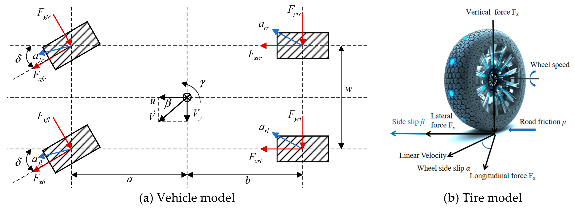
The four-wheel independent drive (4WID) vehicle dynamics model and Dugoff tire model are illustrated in Figure 1. Differential equations of the vehicle body motion are then established to estimate the road adhesion coefficient and tire force.

The differential equations of the vehicle model are:

(1)

Longitudinal movement

$$(F_{xfl}+F_{xfr})\cos \delta -(F_{yfl}+F_{yfr})\sin \delta +F_{xrl}+F_{xrr}=m{a}_x$$

(1)

(2)

Lateral movement

$$(F_{xfl}+F_{xfr})\sin \delta +(F_{yfl}+F_{yfr})\cos \delta +F_{yrl}+F_{yrr}=m{a}_y$$

(2)

(3)

Yaw motion

$$\begin{array}{l}((F_{xfr}-F_{xfl})\cos \delta +(F_{yfl}-F_{yfr})\sin \delta )\frac{a}{2}+((F_{xfl}+F_{xfr})\sin \delta \\ +(F_{yfl}+F_{yfr})\cos \delta )a-(F_{xrl}-F_{xrr})\frac{b}{2}-(F_{yrl}+F_{yrr})b=I_z\dot{\psi }\end{array}$$

(3)

where $a_x$, $a_y$ are longitudinal acceleration and lateral acceleration, respectively, $\delta$ denotes the front left wheel angle, $u$, $V_y$ are the longitudinal and lateral speeds of the vehicle, respectively, $m$ is the vehicle mass, $\psi$ is yaw rate, $fl$, $fr$, $rl$, $rr$ are the left front wheel, right front wheel, left rear wheel, and right rear wheel of the vehicle, respectively, $F_x$, $F_y$ are the longitudinal and lateral forces of the tire, respectively, $a$, $b$ are the distance from the center of mass to the front and rear axles, respectively, and $I_z$ is the moment of inertia around the axis.

The wheel speed and angle can be measured by the built-in sensor of the hub motor. The equations of wheel motion are as follows [38,39]:

$$V_{fl}\cos ({\delta }_{fr})=u-t_f\dot{\psi }$$

(4)

$$V_{fr}\cos ({\delta }_{fl})=u-t_f\dot{\psi }$$

(5)

$$V_{rl}=u+t_r\dot{\psi }$$

(6)

$$V_{rr}=u+t_r\dot{\psi }$$

(7)

According to Equations (4)–(8), the longitudinal velocity of the vehicle and yaw rate can be obtained by:

$$u=\frac{V_{rr}+V_{rl}}{2}=\frac{(w_{rr}+w_{rl})R_w}{2}$$

(8)

$$\dot{\psi }=\frac{V_{rr}-V_{rl}}{2t_r}=\frac{(w_{rr}-w_{rl})R_w}{2t_r}$$

(9)

where $V_{fl}, V_{fr}, V_{rl}, V_{rr}$ are the wheel speed of the front left, front right, rear left, and rear right wheel, respectively, R_w is wheel radius, w is the angular velocity of the wheel, ${\delta }_{fl}, {\delta }_{fr}$ are the wheel angle of the front left and front right, respectively.

Under the driving conditions, the longitudinal slip rate of the wheel is:

$${\sigma }_{ij}=1-\frac{v_{ij}}{w_{ij}R}(ij=fl,fr,rf,rr)$$

(10)

The longitudinal and lateral forces of the tire are calculated using the nonlinear Dugoff model:

$$F_x=C_x\frac{\sigma }{1+\sigma }f(\lambda )$$

(11)

$$F_y=C_{\alpha }\frac{\tan (\alpha )}{1+\sigma }f(\lambda )$$

(12)

where $\sigma$ is the wheel slip ratio, $C_x$, $C_{\alpha }$ are the longitudinal stiffness and lateral stiffness of the tire, respectively, $\lambda$ is related to the adhesion coefficient $\mu$, $\mu$ is the road adhesion coefficient, and $\alpha$ is the wheel slip angle. The function $f(\lambda )$ is also defined as:

$$f(\lambda )=\left\{\begin{array}{c}(2-\lambda )\lambda ,\lambda <1\\ 1,\lambda \ge 1\end{array}\right.$$

(13)

$$\lambda =\frac{\mu F_Z(1+\sigma )}{2\sqrt{{(C_x\sigma )}^2+{(C_{\alpha }\tan \alpha )}^2}}$$

(14)

The vertical loads of each tire are:

$$\left\{\begin{array}{c}{F}_{\mathit{zfl}}=\frac{\mathit{mgb}}{2l}-\frac{m{a}_y\mathit{hb}}{t_{f}l}-\frac{m{a}_{x}h}{2l}\\ F_{\mathit{zfr}}=\frac{\mathit{mgb}}{2l}+\frac{m{a}_y\mathit{hb}}{t_{f}l}-\frac{m{a}_{x}h}{2l}\\ F_{\mathit{zrl}}=\frac{\mathit{mga}}{2l}-\frac{m{a}_y\mathit{ha}}{t_{r}l}+\frac{m{a}_{x}h}{2l}\\ F_{\mathit{zrr}}=\frac{\mathit{mga}}{2l}+\frac{m{a}_y\mathit{ha}}{t_{r}l}+\frac{m{a}_{x}h}{2l}\end{array}\right.$$

(15)

where $t_f$, $t_r$ are the wheelbase of the front and rear wheels, respectively, $l$ is the distance between the front and rear axles, F_zij is the vertical force of the tire, $h$ is the height of the center mass, ${\alpha }_{\mathit{ij}}$ is the tire slip angle, $v_{\mathit{ij}}$ is the longitudinal speed of the wheel center, and $w_{\mathit{ij}}$ is the angular velocity of the wheel.

The input signal is measured by the onboard sensor IMU, and the wheel speed sensor (WSS) and wheel angle sensor (WAS), which are built into the hub motor. When estimating the road adhesion coefficient, parameters closely related to the road adhesion coefficient should be found as inputs. According to Equations (1)–(3) and (11)–(15), the functional relationship between road adhesion coefficient μ and vehicle driving state parameters can be determined as follows:

$$\mu =f(w_{fl},w_{fr},w_{rl},w_{rr},{\sigma }_{fl},{\sigma }_{fr},{\sigma }_{rl},{\sigma }_{rr},a_x,a_y,{\alpha }_{fl},{\alpha }_{fr},{\alpha }_{rl},{\alpha }_{rr},{\delta }_{fl},{\delta }_{fr})$$

(16)

Combined with the vehicle dynamics model, the Spearman correlation between input and output was analyzed, and finally, the input and output signals of the neural network were determined. The results of the PCA analysis are shown in Figure 2.

The parameters related to the road adhesion coefficient were analyzed for extracting the main parameters. Therefore, the input to the road adhesion coefficient model is:

$$\mu =[w_{fl},w_{fr},w_{rl},w_{rr},{\sigma }_{fl},{\sigma }_{rl},{\sigma }_{fr},{\sigma }_{rr}]$$

(17)

Two sub-modules of road types were established, and the latest set of data was used to determine the road type through an adhesion coefficient recognition classifier. The judgment standard was $\epsilon$, the smaller one was the road type of this working condition. This solved the problem of low accuracy in the direct calculation of the road adhesion coefficient.

$$\epsilon =\mu -\widehat{\mu }$$

(18)

Similarly, according to Equations (1)–(16), the input of the self-organizing neural network for estimating $F_x$, $F_y$ was:

$$[\delta ,\psi ,u,a_x,a_y,{\alpha }_{fl},{\alpha }_{rl},{\alpha }_{fr},{\alpha }_{rr},\mu ]$$

(19)

The input of the self-organizing neural network for estimating $F_{\mathrm{z}}$ was:

$$[\delta ,\psi ,u,a_x,a_y,{\omega }_{fl},{\omega }_{rl},{\omega }_{fr},{\omega }_{rr},\mu ]$$

(20)

In the simulation experiment and the real car experiment, the same input signal and output signal were used to establish the neural network model. The signals used in the LM-MMSOFNN algorithm are shown in

Table 1. Signals used in the LM-MMSOFNN algorithm.

#	Notation	Description	Value
1	ax	Longitudinal acceleration	m/s2
2	ay	Lateral acceleration	m/s2
3	Ψ	Yaw rate	rad/s
4	δ	The front wheel angle	deg
5	αFL	The wheel slip angle of front left wheel	deg
6	αFR	The wheel slip angle of front right wheel	deg
7	αRL	The wheel slip angle of rear left wheel	deg
8	αRR	The wheel slip angle of rear right wheel	deg
9	u	Longitudinal speed of the vehicle	km/h
10	ωFL	The angular velocity of the wheel	rad/s
11	ωFR	The angular velocity of the wheel	rad/s
12	ωRL	The angular velocity of the wheel	rad/s
13	ωRR	The angular velocity of the wheel	rad/s

.

2.2. Tire Lateral Stiffness and Longitudinal Stiffness

In order to obtain the tire lateral stiffness and longitudinal stiffness of tire 235/55R20 in the real vehicle experiment, experiments were carried out on the tire forces and moment test bench. When the slip rate and slip angle were small, the tire worked in the linear region. The linear tire force model was used to fit the experimental data and calculate the lateral stiffness and longitudinal stiffness of the tire:

$$F_x=C_x\sigma$$

(21)

$$F_y=C_{\alpha }\alpha$$

(22)

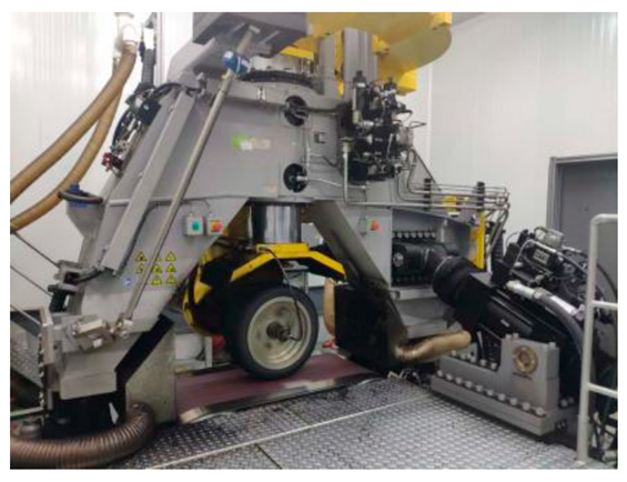
With an inflation pressure of 250 kPa, the full load was 3038 N, and the camber angle continuously changed from −5° to 0° and 5°. There were 12 working conditions in each group, as shown in

Table 2. Tire force pure longitudinal slip test conditions.

Velocity	Load (N)	Slip Rate	Slip Angle
60 km/h	1215.2 (N)	−30–30%	0°
60 km/h	2430.4 (N)	−30–30%	0°
60 km/h	3645.6 (N)	−30–30%	0°
60 km/h	4860.8 (N)	−30–30%	0°

and

Table 3. Tire force pure cornering test conditions.

Velocity	Load	Slip Rate	Slip Angle
60 km/h	40%	free scrolling	−15°–15°
60 km/h	80%	free scrolling	−15°–15°
60 km/h	120%	free scrolling	−15°–15°
60 km/h	160%	free scrolling	-15°-15°

. Figure 3 shows the tire force and moment test bench, and the test results are shown in Figure 4 and Figure 5.

The tire force experimental data could fit the longitudinal and lateral stiffness of the tire. This was conducive to establishing a more accurate vehicle model.

CarSim is a simulation software specifically for vehicle dynamics. It has been adopted by many international automobile manufacturers and has become the standard software in the automobile industry. It can import the real parameters of the experimental vehicle into the CarSim software, set different working conditions, and use the data output of the CarSim to verify the proposed method. The vehicle parameters are listed in

Table 4. Main parameters of the 4WID vehicle.

Variable Parameters	Notation	Description	Value
Mass of the vehicle	m	1412	kg
Moment of inertia around the Z-axis	Iz	1536.7	kg·m2
Distance from the center of mass to the axle	a	1015	mm
Distance from the center of mass to the middle axle	b	1895	mm
Distance from the center of mass to ground	c	540	mm
Wheelbase	W	1675	mm
Wheel effective radius	r	353	mm
Lateral stiffness of the front wheel	cαf	34.4	kN·rad−1
Lateral stiffness of the rear wheel	cαr	30.2	kN·rad−1

.

3. LM-MMSOFNN Algorithm for Identification of Three-Way Tire Forces

3.1. Self-Organizing Feedforward Neural Networks (SOFNN)

In order to meet the demands of online computing, the LM method was selected to improve the computing performance of self-organizing neural networks. The multi-module neural network can calculate the three-way tire force of four wheels at the same time, which also reduces the online running time of the system. The self-organizing neural network automatically finds the internal rules in the samples by adaptively changing the network structure parameters. Therefore, the self-organizing neural network has stronger adaptability to different road types and driving speeds, and higher estimation accuracy than other methods. This can not only preserve the topological mapping between the samples, but it can also reduce the dimension of input feature space and improve computational efficiency. Due to the excellent performance of self-organizing neural networks in classification and prediction, it has strong advantages in the field of road adhesion coefficient recognition and tire force estimation.

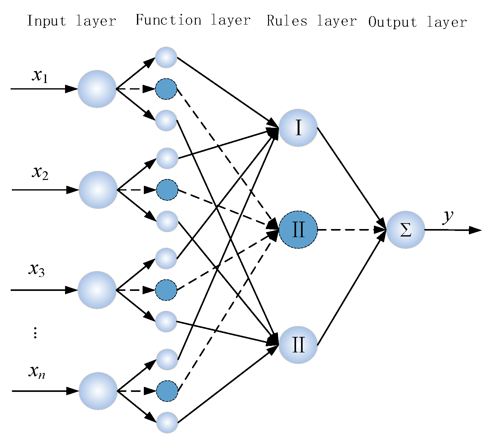
The road adhesion coefficient was calculated first, and then the tire forces of four tires were estimated using SOFNN. The self-organizing network structure was composed of a four-layer network composed of an input layer, a membership function layer, an adaptive rule layer, and an output layer (Figure 6)

3.2. Improved LM Learning Algorithm

The parameters of a self-organizing neural network included the center, $c_{ij}$, and width, ${\sigma }_{ij}$ in the second layer, the weight matrix between the second and third layers, ${\mathrm{W}}^{L1}$, and the weight matrix between the third and fourth layers, ${\mathrm{W}}^{L2}$. In the learning of layer 2, for the online modeling of FNN, the expected target value was: $\mathrm{d}={[d_1,d_2,\cdots ,d_k,\cdots ,d_n]}^T$, and the output target value was $\mathrm{y}={[y_1,y_2,\cdots ,y_k,\cdots ,y_n]}^T$. A single sample was sent to the network for training, and the error $e_n$ was:

$$e_n=d_k-y_k$$

(23)

where $n$ indicates the sample number. The Jacobian matrix $j_p$ was expressed as:

$$j_p=\left[\frac{\partial e_p}{\partial w_1},\cdots ,\frac{\partial e_p}{\partial w_m},\frac{\partial e_p}{\partial c_{11}},\cdots ,\frac{\partial e_p}{\partial c_{nm}},\frac{\partial e_p}{{\partial }_{\sigma 11}},\cdots ,\frac{\partial e_p}{{\partial }_{{\sigma }_{nm}}}\right]$$

(24)

The gradient sub-vector ${\eta }_p$ and sub-matrix $q_p$ were obtained according to Equations (10) and (11).

$${\eta }_p=j_p{e}_p$$

(25)

$$q_p=j_p^{\mathrm{T}}{j}_p$$

(26)

It was seen that the improved LM algorithm only generated row vectors $j_p$, thus avoiding the multiplication of the Jacobian matrices in the algorithm. This reduced the storage space and improved the running speed. For all the training samples in the current sliding window, the gradient vector $g$ and Hessian matrix $Q$ were calculated by cyclic accumulation:

$$g={\displaystyle \sum _{p=1}^P{\eta }_p}$$

(27)

$$Q={\displaystyle \sum _{p=1}^P{q}_p}$$

(28)

The parameter update of the improved LM algorithm was based on:

$$\mathsf{\Phi }(t+1)=\mathsf{\Phi }(t)+{(Q(t)+\mu I)}^{-1}g(t)$$

(29)

where $\mathsf{\Phi }=[w_1,\cdots ,w_m,c_{11},\cdots ,c_{nm},{\sigma }_{11},\cdots ,{\sigma }_{nm}]$. Finally, substituting (13) and (14) into (15) realized online learning of the parameters.

3.3. SOFNN Growth

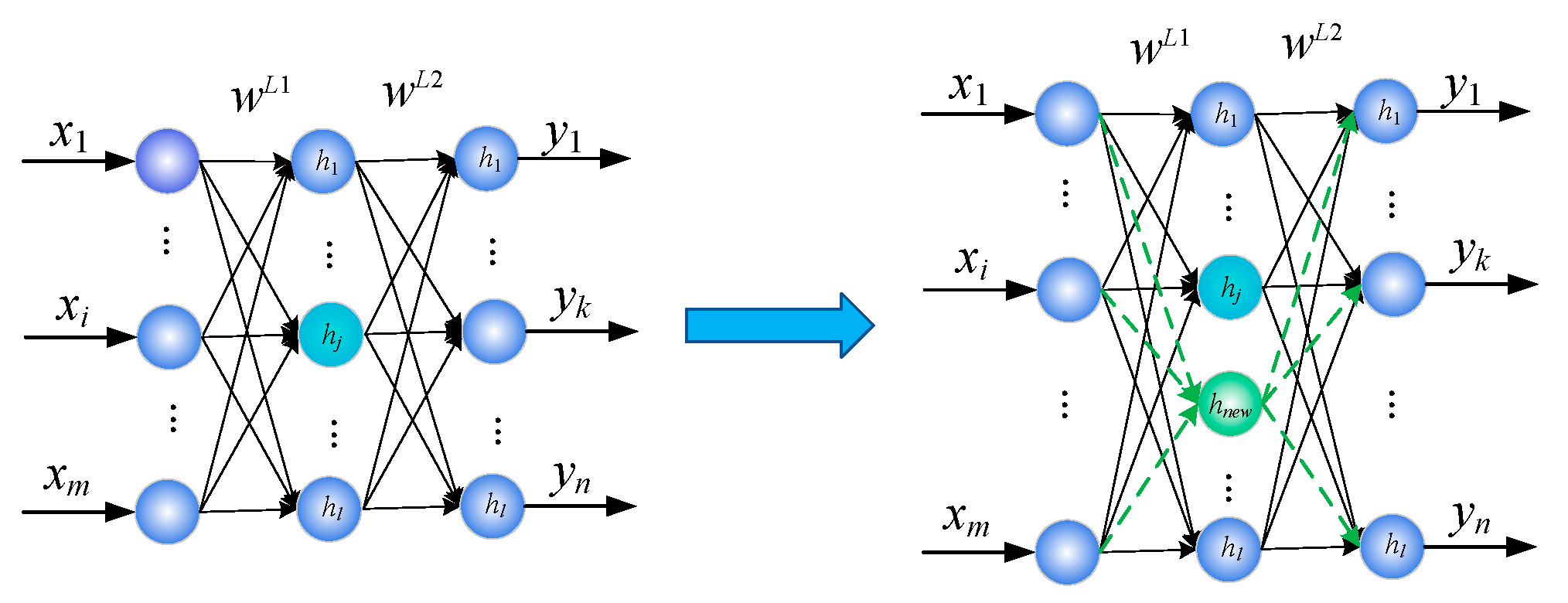
The number of input and output neurons in SOFNN was determined by the training samples, while the number of hidden layer neurons had a great impact on the network structure. Having too many neurons might increase the complexity of the network, whereas fewer neurons might reduce the nonlinear fitting ability of the network [40]. Therefore, the appropriate network structure was required to ensure the computational efficiency of the network while ensuring the required accuracy of tire force estimation. The growth process of the neurons of SOFNN is shown in Figure 7.

In Figure 7, $h_j^{out}$ is the output neuron in the regular layer, and T denotes the total number of learning samples. For a large number of samples or online learning, T is obtained using a sliding window.

The neuron growth index with NGI for SOFNN was:

$${\mathrm{NGI}}_j=\frac{1}{Tn}{\displaystyle \sum _{t=1}^T{\displaystyle \sum _{k=1}^n\frac{w_{jk}^{L2}(t)h_j^{out}(t)}{y_k(t)}}}$$

(30)

and ${\mathrm{G}}_{th}$ was the threshold for the adaptive growth of SOFNN neurons:

$${\mathrm{G}}_{th}=\frac{e^{l/\max l}}{\alpha l}{\displaystyle \sum _{j=1}^l{\mathrm{NGI}}_j}$$

(31)

where $l$ is the number of hidden neurons before growth, $\max l$ is the upper bound of hidden layer neurons, and $\alpha$ is the adaptive growth coefficient, with a value range of (0,1]. During the growth process, a new neuron was added if the j_th hidden neuron NGI_j > G_th.

3.4. SOFNN Pruning

The neural pruning index NPI was defined based on the output variance and output mean of the nodes in the rule layer:

$${\mathrm{NPI}}_j=\sqrt{(\frac{1}{T}{\displaystyle \sum _{t=1}^T{(h_j^{out}(t)-\overline{h_j})}^2})}(\frac{1}{T}{\displaystyle \sum _{n=1}^T{h}_j^{out}(t)})$$

(32)

Combining NPI, we also determined the neuron pruning threshold, ${\mathrm{P}}_{\mathrm{th}}$ to be:

$${\mathrm{P}}_{\mathrm{th}}=e^{l/\max l}\frac{\beta }{l}({\displaystyle \sum _{j=1}^l{\mathrm{NPI}}_j})$$

(33)

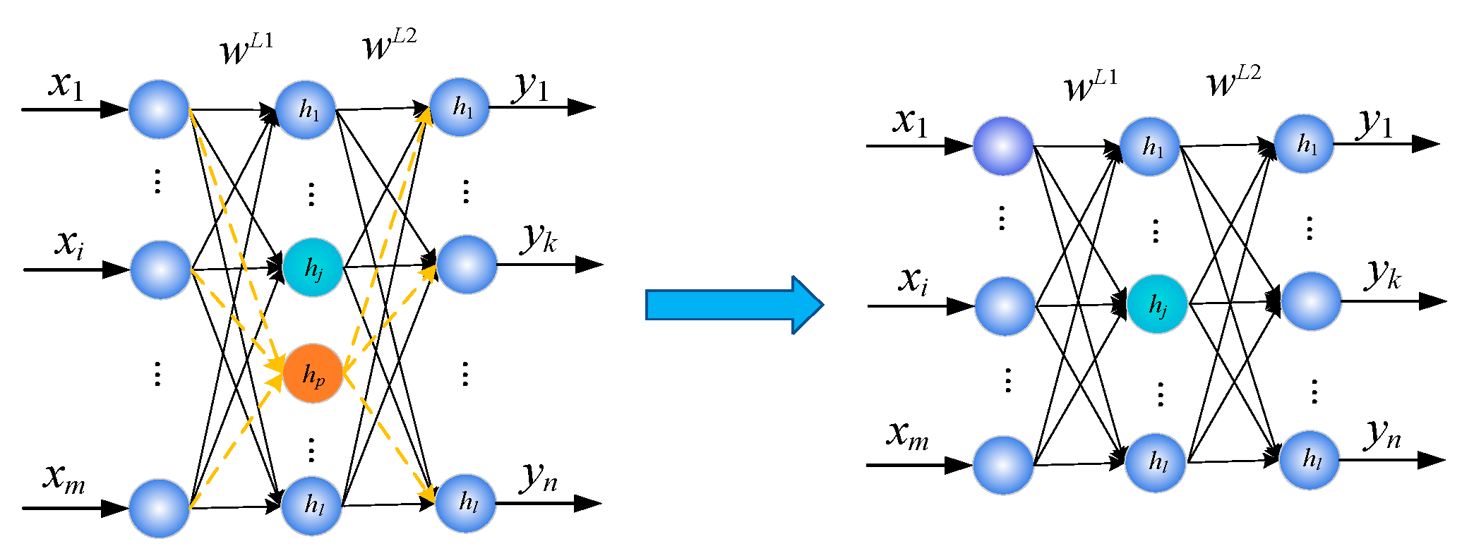
where $\beta$ is the adaptive pruning coefficient, with a value range of (0,1]. The pruning process of SOFNN is shown in Figure 8.

In the process of neuronal modification, if the j_th hidden neuron NPI_j < ${\mathrm{P}}_{\mathrm{th}}$, then the j_th neuron contributed very little to the network; hence, this neuron is pruned off.

3.5. Road Recognition and Tire Force Estimation

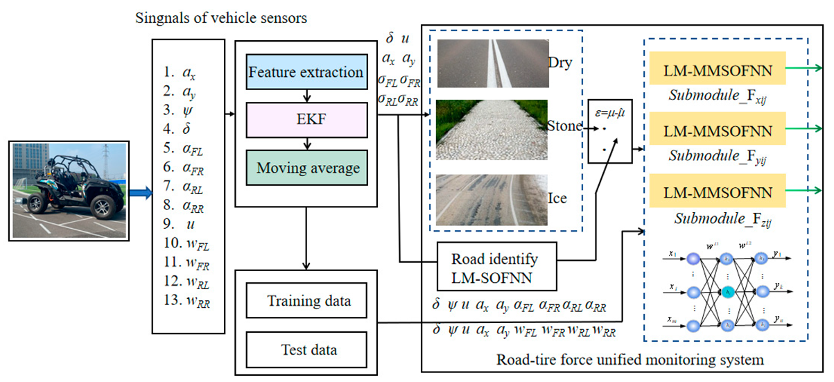
The method based on the LM-MMSOFNN algorithm estimates the tire forces in three directions simultaneously online, which solves the problem that the front and rear lateral forces of the tire cannot be calculated by the same formula when the vehicle turns. Torque can be adjusted according to the actual situation, to achieve accurate stability control of the vehicle, and the slip ratio, road type, and tire forces in each wheel are estimated independently. The LM-MMSOFNN algorithm is designed to estimate the road adhesion coefficient and the data used for model training and testing are collected in real time. When we added multiple neural network sub-models, the classifier selected the one with the lowest error road type. This improved the accuracy of the pavement adhesion coefficient estimation and further improved the accuracy of the tire force estimation. At the same time, the modular design reduced the calculation time and improved the adaptability of online estimation in practical applications. The improved LM, EKF, and MA algorithms and the increase or decrease of self-organizing neurons reduced the computational complexity and the required storage capacity. This algorithm included three parts:

(1)

The noise of the measurement signal was reduced through the Extended Kalman Filter (EKF) and Moving Average.

(2)

The LM-MMSOFNN algorithm was designed to estimate the road adhesion coefficient. The road type was then identified through a road adhesion coefficient recognition classifier.

(3)

The multi-module neural network method was then proposed to calculate the longitudinal, lateral, and vertical tire forces of four tires at the same time. The structure is shown in Figure 9.

The three initial road types were set as dry asphalt, gravel road, and ice road, with the initial road adhesion coefficients set as 0.85, 0.6, and 0.25. When the actual vehicle is driving, the road adhesion coefficients estimated by the neural network will select the closest road type in the classifier, which reduces the estimation error of the road adhesion coefficient and improves the stability of the network and adaptability to different road conditions. Note that the smaller the interval of adhesion coefficients in the initial road type classification, the higher accuracy of final adhesion coefficients obtained, and the estimation of tire force will also be more accurate.

4. Simulation and Vehicle Tests

4.1. Simulation Results

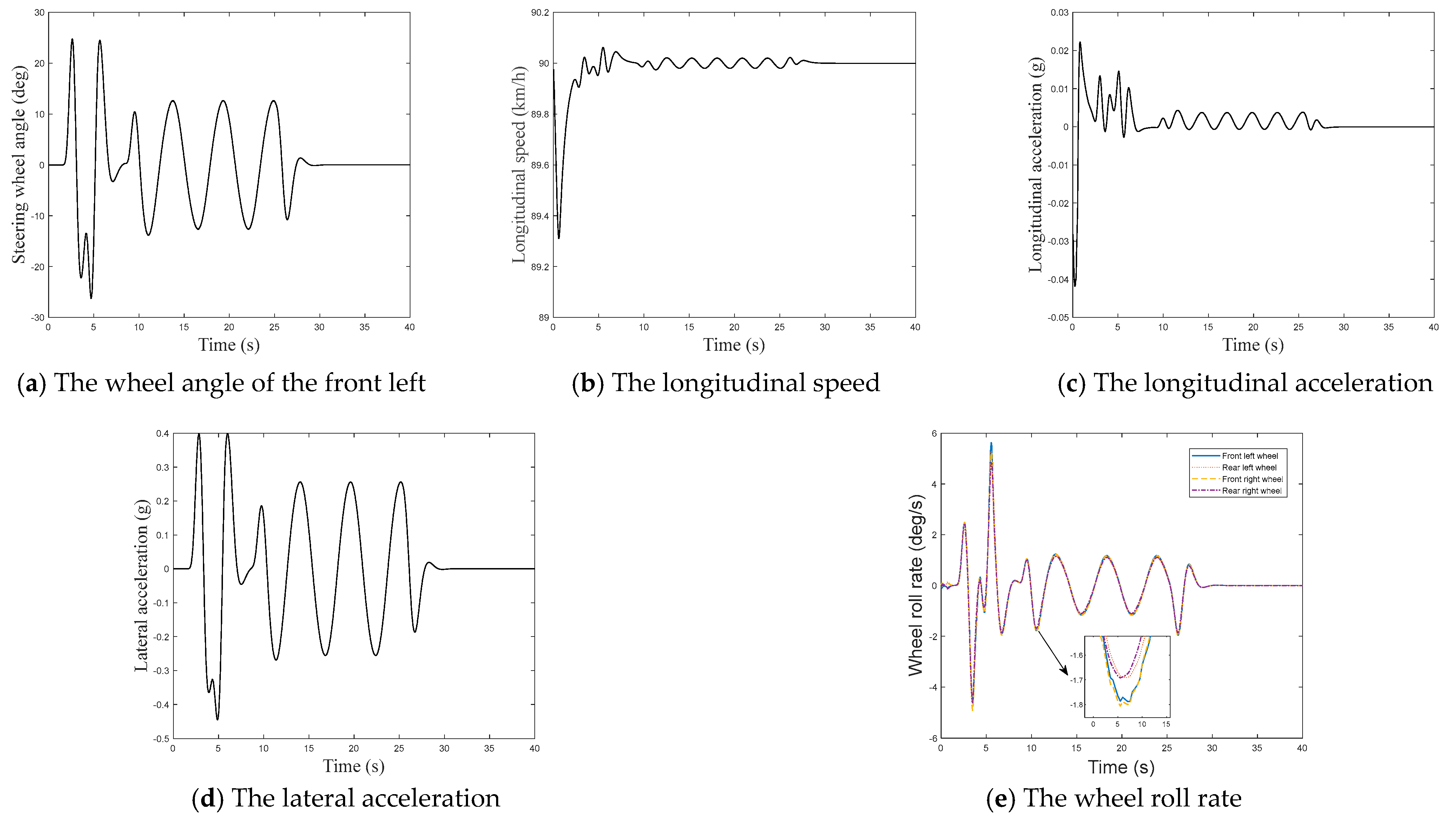
To verify the effectiveness of the proposed LM-MMSOFNN road and tire integrated monitoring method, CarSim was used to generate dynamic simulation data. The simulation environment conforming to the actual vehicle was set in the CarSim software, including the relevant parameters of the test vehicle, to establish the vehicle model. Experimental conditions were set, including vehicle speed, road adhesion coefficient, driving track, driving start and stop time, etc. A series of vehicle driving data is then generated. The speed was set at 90 km/h, and the road adhesion coefficient was 0.85 (i.e., dry asphalt road). The cars first drove for 10 s on a double-lane road, then 20 s on the serpentine road. Secondary feature extraction was carried out to remove unavailable data, and 3200 sets of data were finally obtained for neural network modeling. This data contained the values of all input and output signals.

The secondary feature extraction of the data processing can reduce the learning time of the neural network and avoid the overfitting problem. Then the data is divided into a training set of 70% and a test set of 30%. After the network is designed and trained, the algorithm is deployed to the Rapid Control Prototype control unit on the vehicle for experimental verification. RCP is a real-time target control system developed by Speedgoat Company. It is officially recommended by MathWorks to realize real-time online development in the Simulink environment. Through a combination of CarSim and Simulink, real-time road adhesion coefficient and tire force estimation can be realized. The parameters that can be measured by the vehicle are shown in Figure 10.

For the performance evaluation index, we considered RMSE, MAE, and NRMS (normalized root mean square error) [25]:

$$\mathrm{NRMS}=\frac{\sqrt{{\displaystyle \sum _{i=1}^N{(F_{ij}-{\widehat{F}}_{ij})}^2/N}}}{\max (|F_{ij}|)}$$

(34)

$$\mathrm{RMSE}=\sqrt{\frac{1}{N}{\displaystyle \sum _{i=1}^N{(F_{ij}-{\widehat{F}}_{ij})}^2}}$$

(35)

$$\mathrm{MAE}=\frac{1}{N}{\displaystyle \sum _{i=1}^N|F_{ij}-{\widehat{F}}_{ij}}|$$

(36)

In order to analyze the safe operating range of the vehicle, LTR can be calculated by:

$$\mathrm{LTR}=\frac{F_{zfl}+F_{zrl}-F_{zfr}-F_{zrr}}{F_{zfl}+F_{zrl}+F_{zfr}+F_{zrr}}$$

(37)

where, $F_{zfl}$, $F_{zrl}$, $F_{zfr}$, $F_{zrr}$ are the vertical forces of the left front wheel, the right front wheel, the left rear wheel, and the right rear wheel, respectively. The LTR index ranges from −1 to 1, and when it is close to 0, the left and right sides of the vehicle have the same vertical load, with strong stability and no possibility of rollover. If LTR is near to ±1, the vehicle can easily roll over. This is because the proposed tire force estimation method can only be used when the vehicle is in a steady state. That is, the threshold value of LTR is set to 0.8.

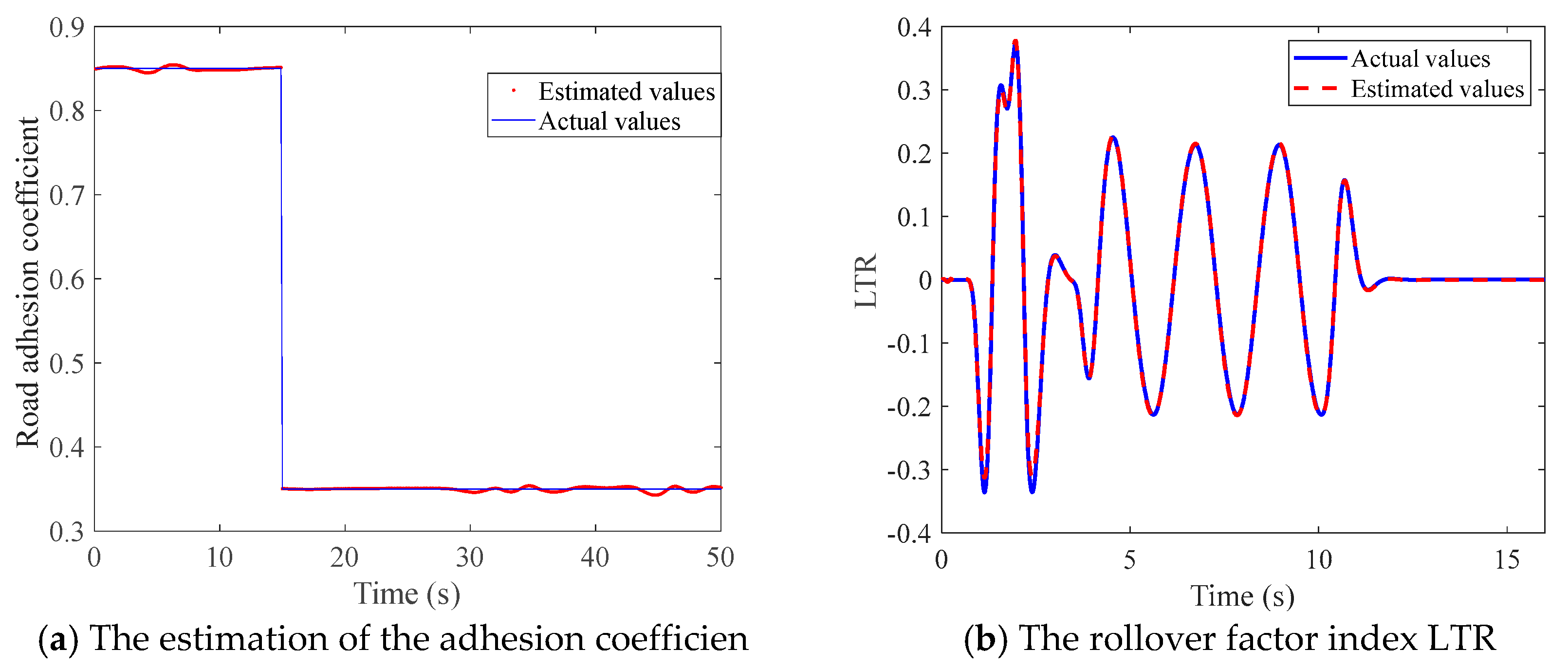
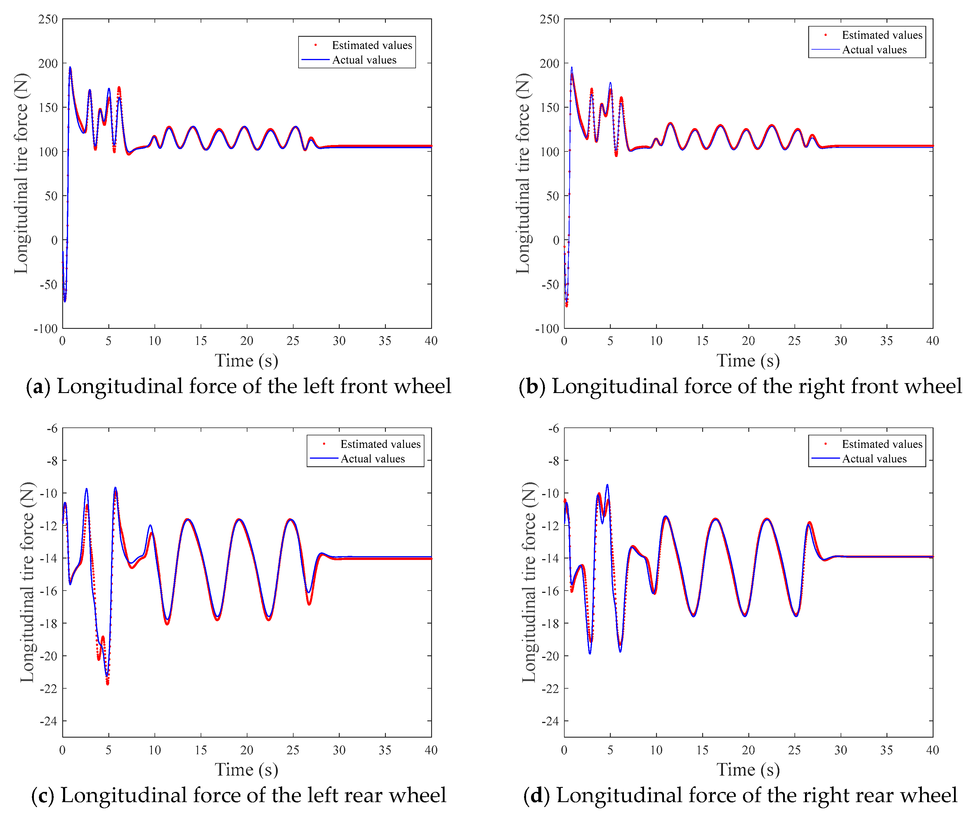
At a speed of 90 km/h, the vehicle was driven on a dry asphalt road with an adhesion coefficient of 0.85 for 15 s and then led to an ice and snow road with an adhesion coefficient of 0.35. Using the integrated monitoring method of LM-MMSOFNN, the road adhesion coefficient and tire forces of the four wheels are shown in Figure 11, Figure 12, Figure 13 and Figure 14.

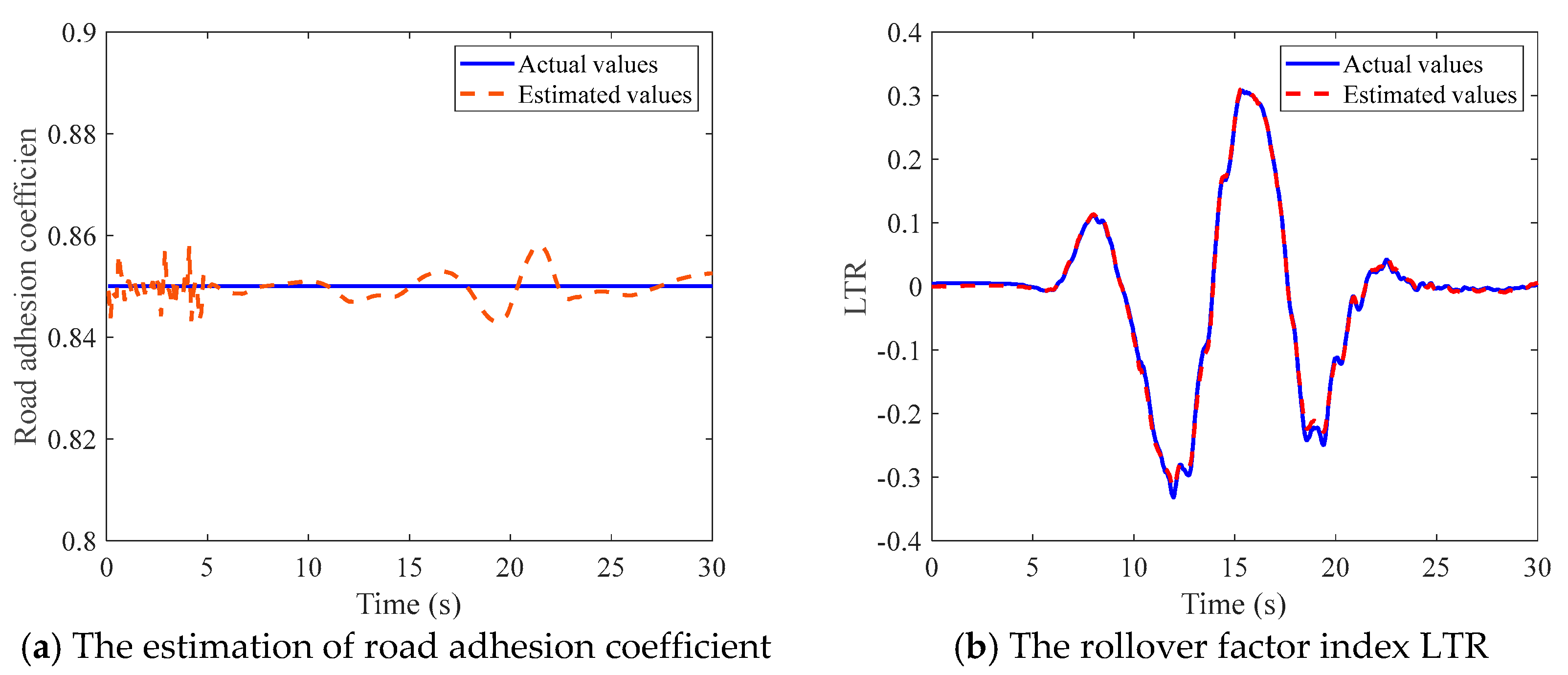
It can be seen from Figure 11a that the estimation of the road adhesion coefficient was highly accurate, with an MAE value of 0.0163. Therefore, this method can provide a basis for accurate identification of the road type. Figure 11b describes that in the simulation test of snake driving on dry asphalt and ice road conditions, the roll-factor index LTR always remained below 0.38. Therefore, there was no rollover risk in this driving condition. The effective methods to reduce LTR were premature braking and quick front wheel alignment. LTR was directly proportional to the quadratic longitudinal speed. Therefore, at high speed, with the support of the Electronic Power Steering (EPS) system, early braking can effectively reduce the LTR and reduce the vehicle rollover risk.

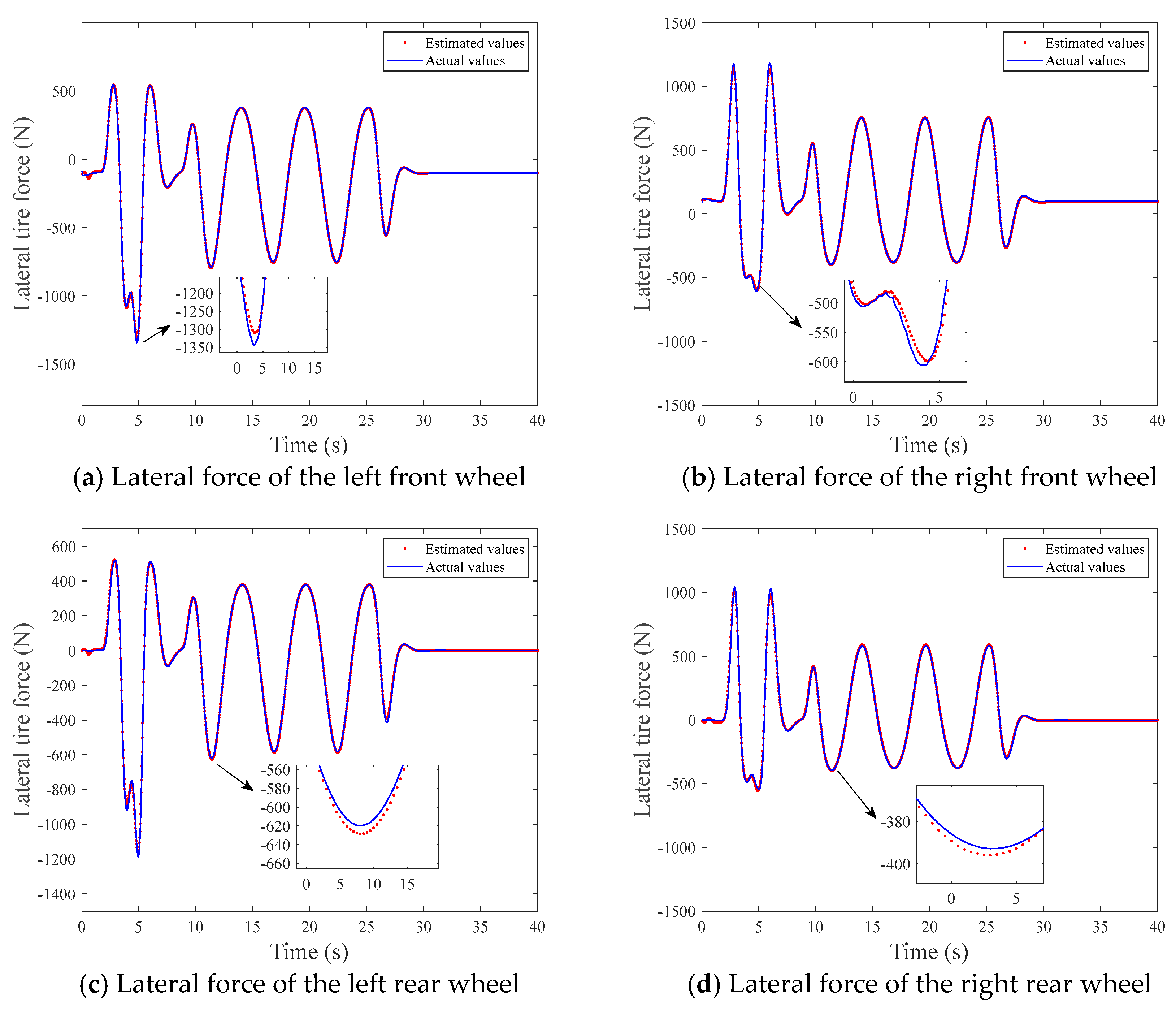
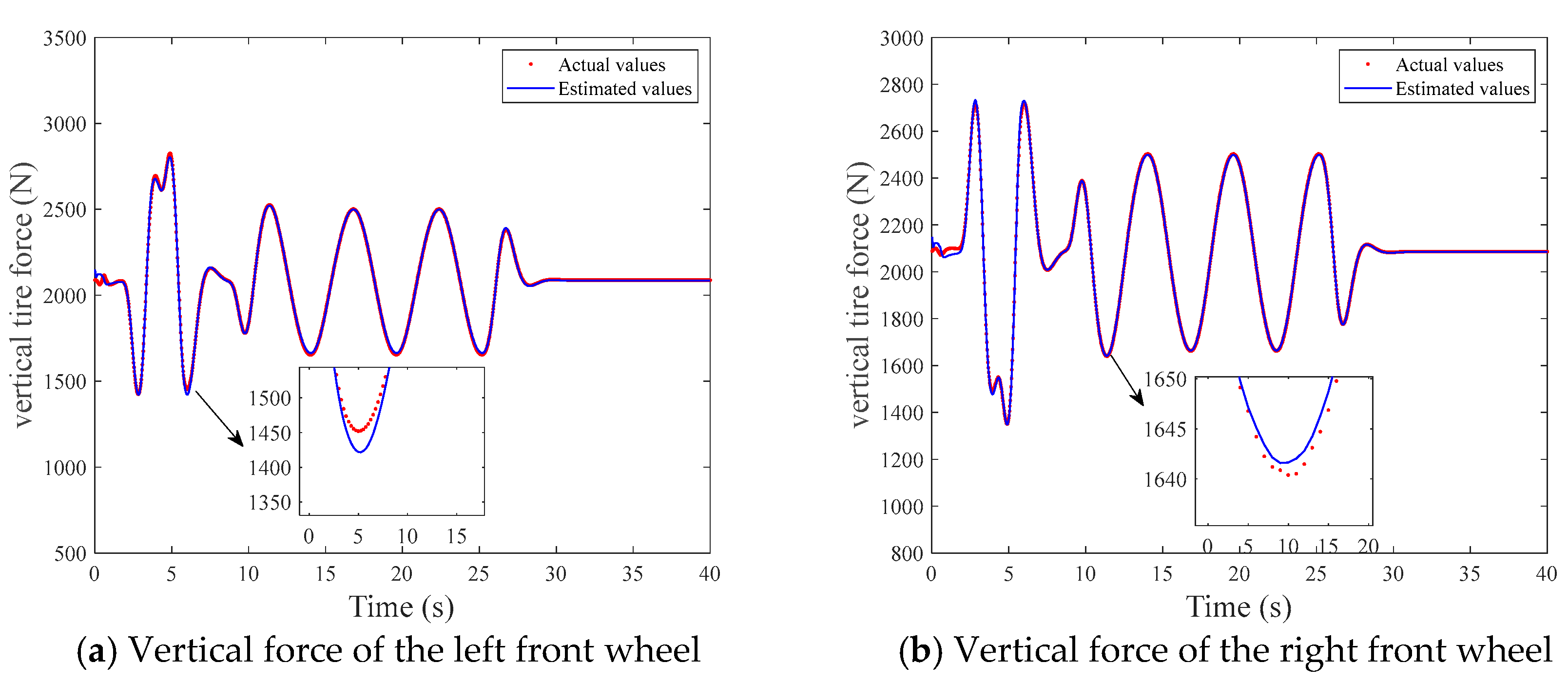
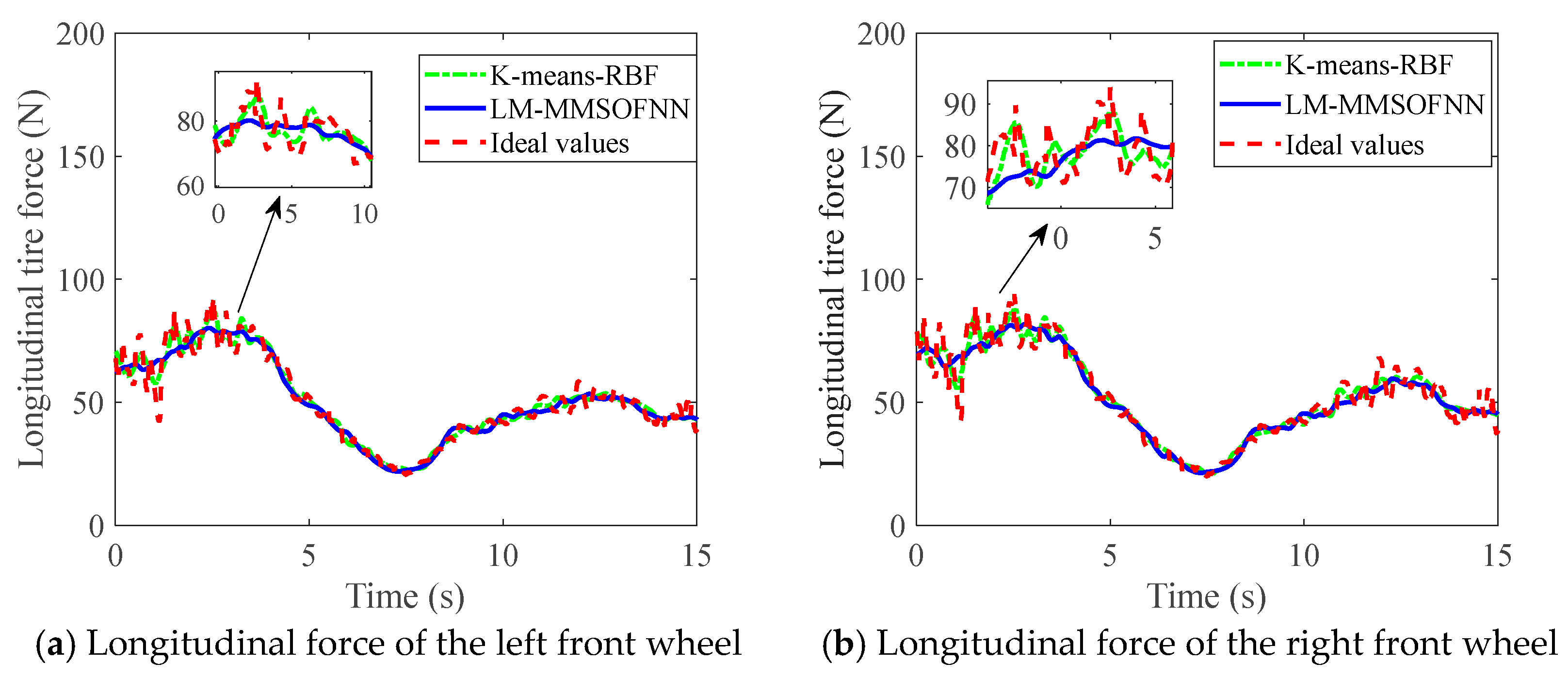
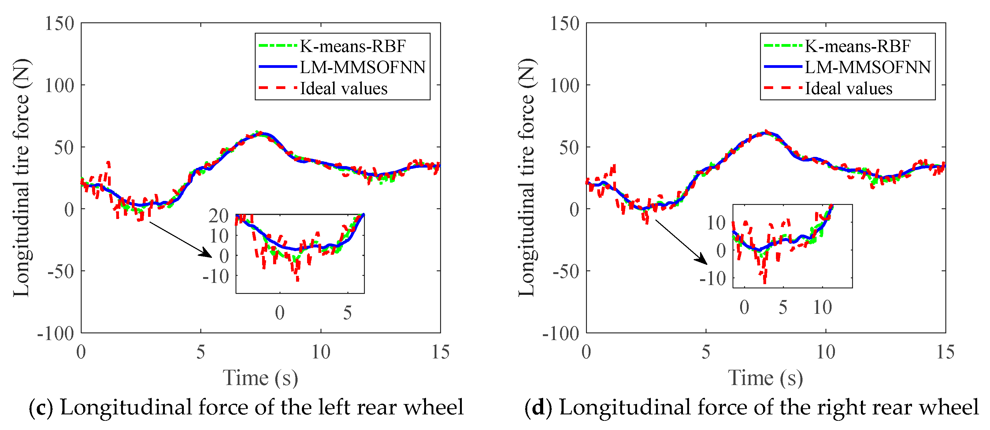
Figure 12 shows the longitudinal tire force estimation results of each wheel in a complex scenario. During frequent cornering and driving, the maximum tire force of the front wheels was 190 N and the maximum tire force of the rear wheels was 21 N. Figure 13 also shows that the lateral tire force estimation of the wheels was highly accurate during the steering operation. Furthermore, Figure 14 shows that during the estimation process, the vertical tire force was affected by a vertical vibration transient response. Therefore, it was necessary to eliminate the unstable data before 0.25 s to improve the estimation accuracy. The initial position of the neural network was random, which resulted in different estimations at each time. We further compared the average value of five calculation results with that presented in

Table 5. The longitudinal force estimation error.

	Fxfl	Fxfr	Fxrl	Fxrr
NRMS (%)	2.31	4.18	2.51	4.22
NRMS(%)[25]	5.16	4.44	7.07	7.07
RMSE(N)	0.21	0.39	0.24	0.40
MAE(N)	0.12	0.24	0.14	0.22

,

Table 6. The lateral force estimation error.

	Fyfl	Fyfr	Fyrl	Fyrr
NRMS (%)	1.26	2.31	0.79	0.87
NRMS(%)[25]	9.3	7.2	13.54	11.25
RMSE(N)	6.91	12.03	9.32	9.10
MAE(N)	3.92	7.10	4.88	6.62

and

Table 7. The vertical force estimation error.

	Fzfl	Fzfr	Fzrl	Fzrr
NRMS (%)	1.34	1.27	1.28	1.33
NRMS(%)[25]	5.37	5.17	7.00	6.80
RMSE(N)	6.78	9.10	7.73	8.80
MAE(N)	3.67	5.79	4.85	5.14

.

The longitudinal, lateral, and vertical tire forces estimated by LM-MMSOFNN were highly accurate and the corresponding maximum MAE and RMSE were 7.1 N and 12.03 N, respectively. The estimation of NRMS was smaller, which verified the effectiveness of the proposed algorithm.

4.2. Real Vehicle Tests

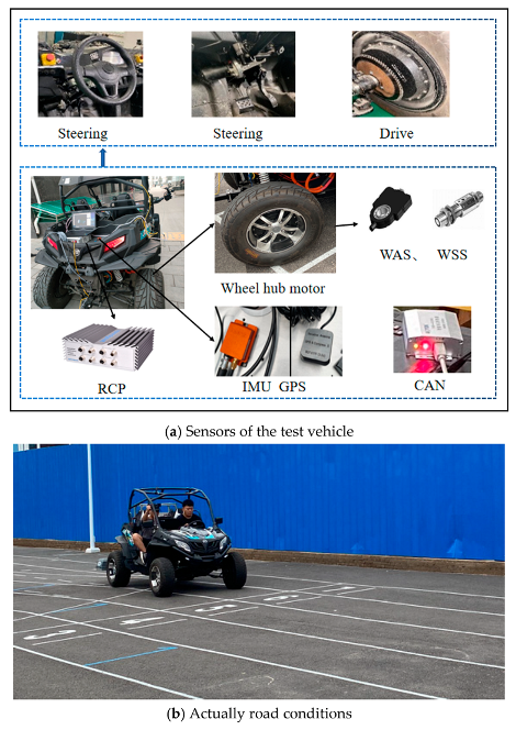
The experiment was carried out with a four-wheel independent distributed drive pure wire controlled intelligent vehicle. The type of inertial measurement unit (IMU) of the vehicle was MTI-G-710, which measured longitudinal acceleration, lateral acceleration, yaw rate, and vehicle longitudinal speed. The sampling period of the global positioning system (GPS) was 2.5 ms. Rapid control prototype (RCP) is a real-time target control system developed by Speedgoat which is recommended by MathWorks and can realize real-time online development in the Simulink environment. The wheel speed sensor (WSS) and wheel angle sensor (WAS) were built into the hub motor which measured the wheels’ speeds and roll rate, then transmitted to the computer through the CAN bus, and the command cycle was 10ms. In this real serpentine experiment, the road adhesion coefficient was 0.85, and a total of 14,368 sets of data were obtained through sensor measurements. Then the data was divided into a training set of 70% and a test set of 30%. The experimental vehicle sensors and actual test road conditions are shown in Figure 15.

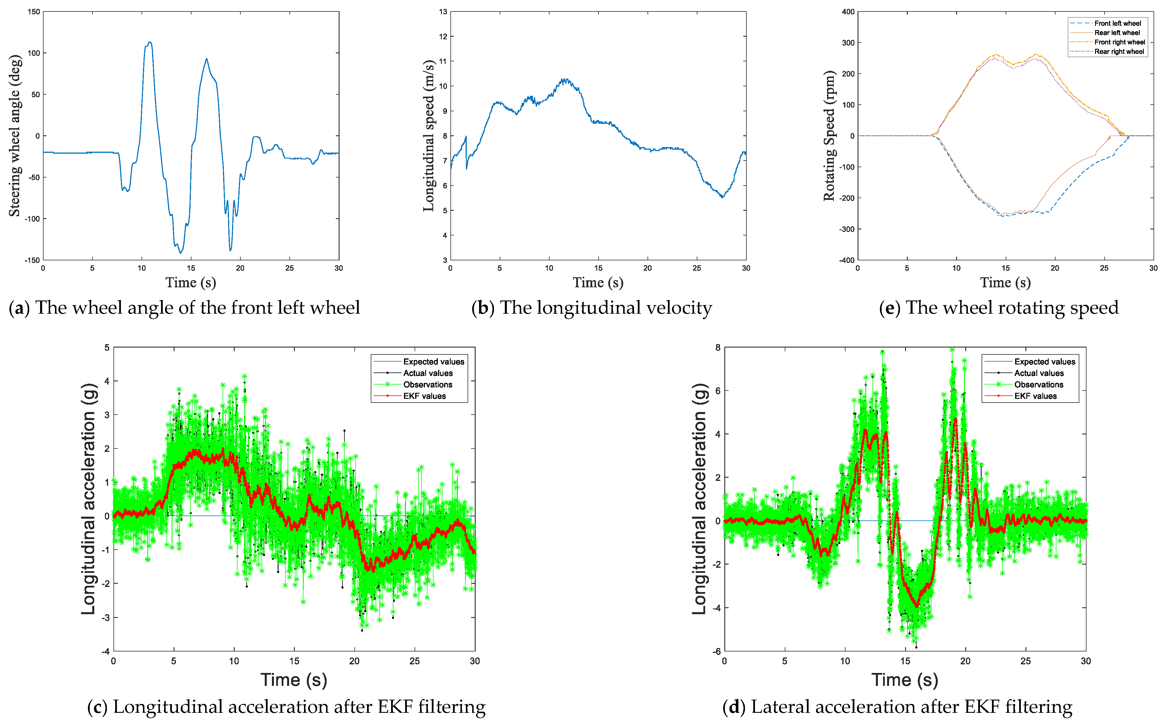
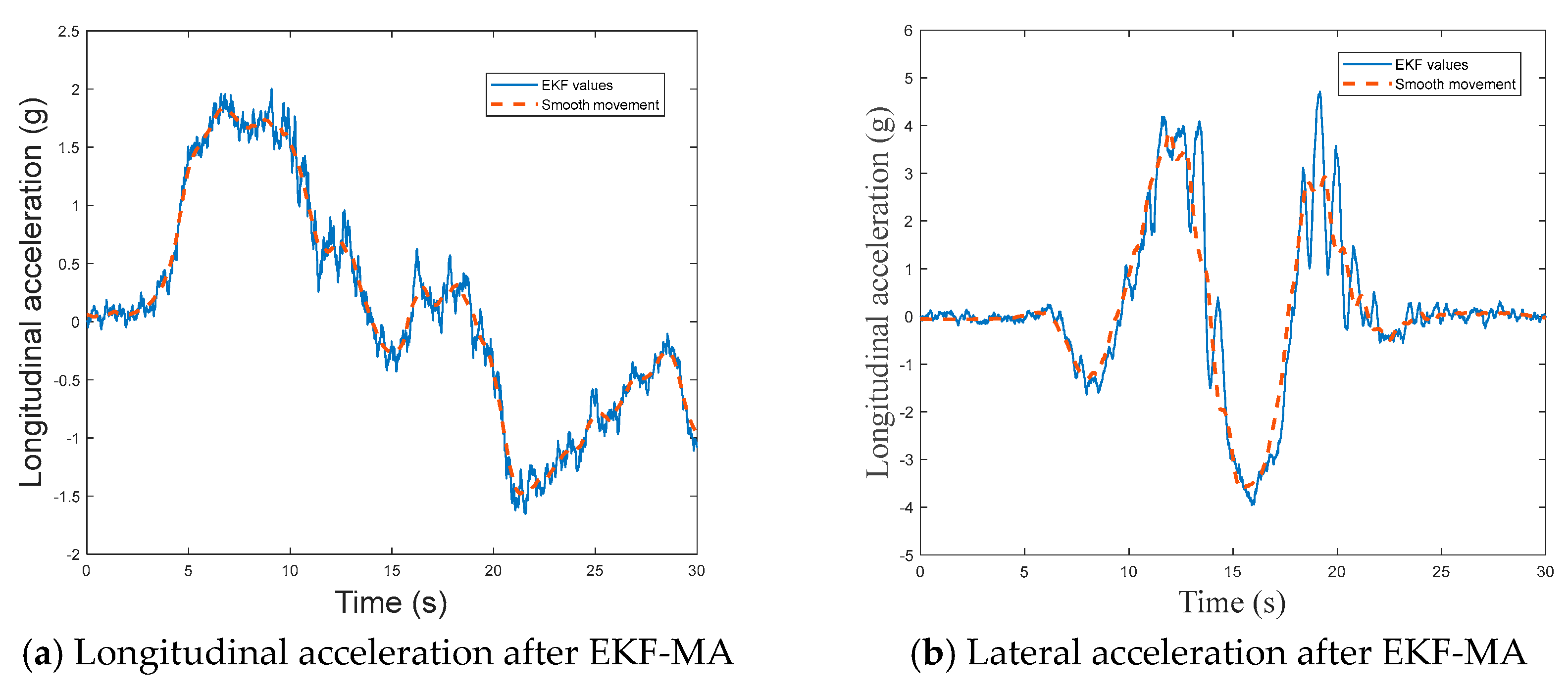
The actual vehicle test was carried out under dry asphalt road conditions. The data measured by the sensor of the vehicle included longitudinal acceleration, lateral acceleration, longitudinal velocity, the wheel angle, and the wheel rotating speed, as shown in Figure 16. Due to the large measurement noise in IMU, the measured longitudinal acceleration and lateral acceleration were processed by the EKF to reduce the impact of the road adhesion coefficient and the tire force estimation.

Figure 16c,d shows that the waveform after EKF filtering was still not completely smooth. To reduce the system operation time and improve the estimation accuracy, MA (Moving Average) was introduced to smooth the measured longitudinal and lateral acceleration signals. Through multiple experiments, the window length was determined to be 100. The longitudinal and lateral accelerations filtered by the EKF-MA method are shown in Figure 17.

Using LM-MMSOFNN, the road adhesion coefficient and tire force of the four wheels were obtained and are shown in Figure 18, Figure 19, Figure 20 and Figure 21. The estimation errors of LM-MMSOFNN and K-means-RBF are the average of five calculations (see

Table 8. Longitudinal tire force estimation errors of LM-MMSOFNN and K-means-RBF.

		Fxfl	Fxfr	Fxrl	Fxrr
LM-MMSOFNN	NRMS(%)	4.60	5.35	6.84	6.61
	RMSE(N)	4.26	5.02	4.23	4.18
	MAE(N)	2.97	3.45	2.93	2.95
K-means-RBF	NRMS(%)	13.49	12.57	12.38	13.77
	RMSE(N)	16.49	16.07	16.74	14.86
	MAE(N)	8.95	8.91	9.13	8.95

,

Table 9. Lateral tire force estimation errors of LM-MMSOFNN and K-means-RBF.

		Fyfl	Fyfr	Fyrl	Fyrr
LM-MMSOFNN	NRMS(%)	1.68	1.94	0.36	0.35
	RMSE(N)	13.65	14.28	4.25	4.11
	MAE(N)	21.87	22.58	2.94	2.88
K-means-RBF	NRMS(%)	6.48	6.22	5.44	4.87
	RMSE(N)	95.52	87.41	63.59	56.73
	MAE(N)	87.05	73.31	43.63	42.32

and

Table 10. Vertical tire force estimation errors of LM-MMSOFNN and K-means-RBF.

		Fzfl	Fzfr	Fzrl	Fzrr
LM-MMSOFNN	NRMS(%)	0.20	0.27	0.36	0.40
	RMSE(N)	9.02	8.10	8.43	12.71
	MAE(N)	7.35	5.92	6.56	10.65
K-means-RBF	NRMS(%)	1.62	2.19	2.49	1.73
	RMSE(N)	48.47	51.98	77.08	40.24
	MAE(N)	39.31	44.97	64.11	33.56

).

Figure 18a shows the road adhesion coefficient estimation of LM-MMSOFNN on a dry asphalt road. The MAE was 0.00154. i.e., it could accurately identify the road type. Note that for identifying new road types, only the neural network sub-modules need to be added. Therefore, this method provides adaptability and convenience to a variety of working conditions. It can be seen from Figure 18b that in the real vehicle test of snake road conditions, the roll-factor index LTR was always at a relatively low index, and there was no rollover risk. LTR increased at acceleration and turning; however, the braking time was shortened to account for the decrease of longitudinal adhesion coefficient during steering. As a result, braking alone was difficult to rapidly reduce the roll-factor index LTR, and combined with steering control improved control effectiveness.

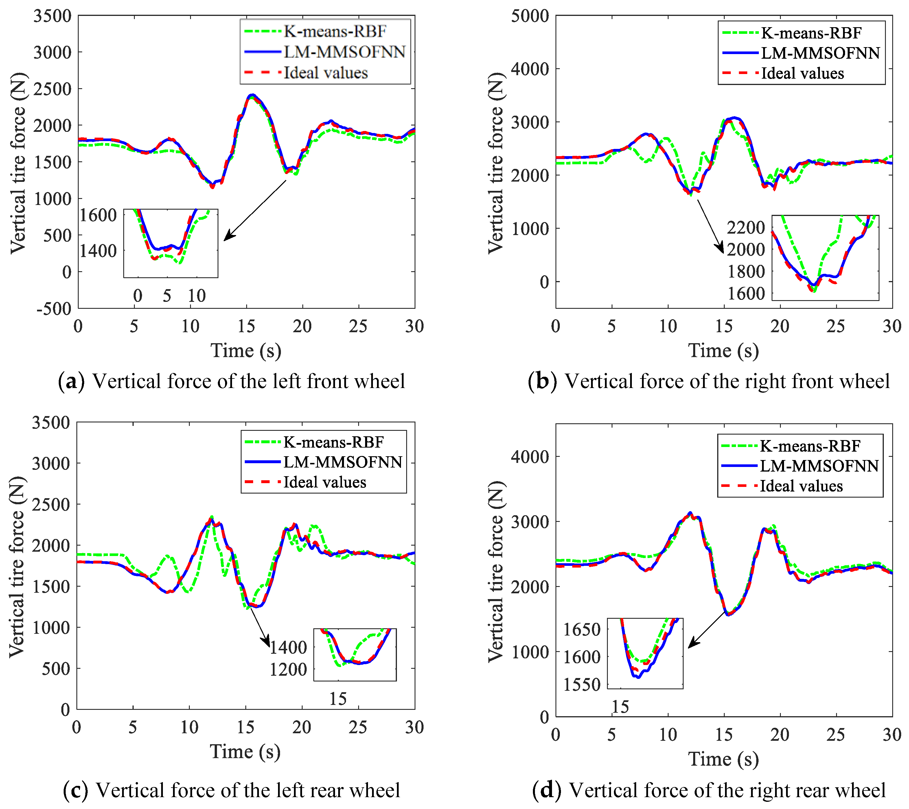
Figure 19 shows the longitudinal tire force of the wheels. Since some of the sensors’ signals might have been out of synchronization or simply missed, the 15 s block is what remained after deleting the blank data. It can be seen from Figure 20 that the front and rear longitudinal tire forces were similar. Due to the side slip, the rear lateral force was smaller than that of the front. In the serpentine condition, the maximum lateral tire force was 60 times of longitudinal tire force. Therefore, the accurate estimation of the lateral tire force could be used for the torque adjustment in the motor, which was helpful for improving the side slip phenomenon. Figure 21 shows the vertical tire force of the wheels. The number of required calculations, as well as noise, was reduced using the EKF-MA method.

Table 8, Table 9 and Table 10 also indicate that for estimating tire force, the integrated estimation of road tire force based on LM-MMSOFNN proposed in this paper had higher estimation accuracy than the K-means-RBF algorithm. The values of NRMS, RMSE, and MAE were all smaller than the K-means-RBF algorithm. The minimum NRMS, RMSE, and MAE were 0.2%, 4.11 N, and 2.88 N.

5. Conclusions

A novel LM-MMSOFNN structure was proposed for road recognition and online three-directional tire forces estimation. A self-organizing neural network was designed to establish the sub-modules required for different types of roads and the road type was then recognized by the road adhesion coefficient recognition classifier. Finally, the tire force estimation sub-modules were used to estimate the tire forces of the wheels. The EKF-MA method was also used for noise reduction and data processing in order to reduce computational complexity and improve estimation accuracy. It can be concluded that:

(1)

The proposed method was able to estimate the road adhesion coefficient and tire forces of each wheel independently and provided a variety of information, facilitating accurate control of the distributed drive vehicles.

(2)

The improved LM self-organize neurons adapted to different road conditions and thus promoted the generalization ability of the network.

(3)

The proposed sub-modules addressed the problem that when the vehicle is turning, the front and rear lateral forces cannot be estimated by a unified formula.

(4)

A more detailed classification of road surface types contributed to the accuracy of the road adhesion coefficient and tire force estimates.

References

1. Urda, P.; Aceituno, J.F.; Muñoz, S.; Escalona, J.L. Artificial neural networks applied to the measurement of lateral wheel-rail contact force: A comparison with a harmonic cancellation method. Mech. Mach. Theory 2020, 153, 103968. [Google Scholar] [CrossRef]
2. Xiong, Y.; Yang, X. A review on in-tire sensor systems for tire-road interaction studies. Sens. Rev. 2018, 38, 231–238. [Google Scholar] [CrossRef]
3. Zareian, A.; Azadi, S.; Kazemi, R. Estimation of road friction coefficient using extended Kalman filter, recursive least square, and neural network. Proc. Inst. Mech. Eng. Part K J. Multi-Body Dyn. 2015, 230, 52–68. [Google Scholar] [CrossRef]
4. Kim, C.; Hahn, J.; Hong, K.; Yoo, W. Estimation of Tire-Road Friction Coefficient Based on On-Board 6-DoF Acceleration Measurement. IEEE Trans. Veh. Technol. 2015, 64, 3368–3377. [Google Scholar] [CrossRef]
5. Rajendran, S.; Spurgeon, S.K.; Tsampardoukas, G.; Hampson, R. Estimation of road frictional force and wheel slip for effective antilock braking system (ABS) control. Int. J. Robust Nonlinear Control. 2019, 29, 736–765. [Google Scholar] [CrossRef] [Green Version]
6. Huang, B.; Fu, X.; Wu, S.; Huang, S. Calculation Algorithm of Tire-Road Friction Coefficient Based on Limited-Memory Adaptive Extended Kalman Filter. Math. Probl. Eng. 2019, 2019, 1–14. [Google Scholar] [CrossRef]
7. Gao, L.; Xiong, L.; Lin, X.; Xia, X.; Liu, W.; Lu, Y.; Yu, Z. Multi-sensor Fusion Road Friction Coefficient Estimation During Steering with Lyapunov Method. Sensors 2019, 19, 3816. [Google Scholar] [CrossRef] [PubMed] [Green Version]
8. Chen, X.; Li, S.; Li, L.; Zhao, W.; Cheng, S. Longitudinal-lateral-cooperative estimation algorithm for vehicle dynamics states based on adaptive-square-root-cubature-Kalman-filter and similarity-principle. Mech. Syst. Signal Process. 2022, 176, 109162. [Google Scholar] [CrossRef]
9. Singh, K.B.; Arat, M.A.; Taheri, S. Literature review and fundamental approaches for vehicle and tire state estimation. Veh. Syst. Dyn. 2018, 57, 1–23. [Google Scholar] [CrossRef]
10. Jin, X.; Yin, G.; Chen, N. Advanced Estimation Techniques for Vehicle System Dynamic State: A Survey. Sensors 2019, 19, 4289. [Google Scholar] [CrossRef] [Green Version]
11. Rajamani, R.; Phanomchoeng, G.; Piyabongkarn, D.; Lew, J.Y. Algorithms for Real-Time Estimation of Individual Wheel Tire-Road Friction Coefficients. IEEE/ASME Trans. Mechatron. 2011, 17, 1183–1195. [Google Scholar] [CrossRef]
12. Anderson, R.; Bevly, D.M. Using GPS with a model-based estimator to estimate critical vehicle states. Veh. Syst. Dyn. 2010, 48, 1413–1438. [Google Scholar] [CrossRef]
13. Wang, Y.; Zhou, Z.; Wei, C.; Liu, Y.; Yin, C. Host-target vehicle model-based lateral state estimation for preceding target vehicles considering measurement delay. IEEE Trans. Ind. Inform. 2018, 9, 4190–4199. [Google Scholar] [CrossRef]
14. Bevly, D.M.; Ryu, J.; Gerdes, J.C. Integrating INS Sensors With GPS Measurements for Continuous Estimation of Vehicle Sideslip, Roll, and Tire Cornering Stiffness. IEEE Trans. Intell. Transp. Syst. 2006, 7, 483–493. [Google Scholar] [CrossRef]
15. Caroux, J.; Lamy, C.; Basset, M.; Gissinger, G.-L. Sideslip angle measurement, experimental characterization and evaluation of three different principles. IFAC Proc. Vol. 2007, 40, 505–510. [Google Scholar] [CrossRef]
16. Yi, J.; Alvarez, L.; Horowitz, R. Adaptive emergency braking control with underestimation of friction coefficient. IEEE Trans. Control. Syst. Technol. 2002, 10, 381–392. [Google Scholar] [CrossRef]
17. Wu, B.-F.; Chang, P.-J.; Chen, Y.-S.; Huang, C.-W. An Intelligent Wheelchair Anti-Lock Braking System Design With Friction Coefficient Estimation. IEEE Access 2018, 6, 73686–73701. [Google Scholar] [CrossRef]
18. Saadeddin, K.; Abdel-Hafez, M.F.; Jaradat, M.A.; Jarrah, M.A. Performance enhancement of low-cost, high-accuracy, state estimation for vehicle collision prevention system using ANFIS. Mech. Syst. Signal Process. 2013, 41, 239–253. [Google Scholar] [CrossRef]
19. Ribeiro, A.M.; Moutinho, A.; Fioravanti, A.R.; de Paiva, E.C. Estimation of tire–road friction for road vehicles: A time delay neural network approach. J. Braz. Soc. Mech. Sci. Eng. 2019, 42, 4. [Google Scholar] [CrossRef] [Green Version]
20. Sun, X.; Gong, S.; Han, G.; Wang, M.; Jin, A. Pruning Elman neural network and its application in bolt defects classification. Int. J. Mach. Learn. Cybern. 2018, 10, 1847–1862. [Google Scholar] [CrossRef]
21. Bonfitto, A.; Feraco, S.; Tonoli, A.; Amati, N. Combined regression and classification artificial neural networks for sideslip angle estimation and road condition identification. Veh. Syst. Dyn. 2019, 58, 1766–1787. [Google Scholar] [CrossRef]
22. Šabanovič, E.; Žuraulis, V.; Prentkovskis, O.; Skrickij, V. Identification of road-surface type using deep neural networks for friction coefficient estimation. Sensors 2020, 20, 612. [Google Scholar] [CrossRef] [Green Version]
23. Marques, F.; Woliński, Ł.; Wojtyra, M.; Flores, P.; Lankarani, H. An investigation of a novel LuGre-based friction force model. Mech. Mach. Theory 2021, 166, 104493. [Google Scholar] [CrossRef]
24. Wilkin, M.A.; Manning, W.; Crolla, D.A.; Levesley, M.C. Use of an extended Kalman filter as a robust tyre force estimator. Veh. Syst. Dyn. 2006, 44, 50–59. [Google Scholar] [CrossRef]
25. Hsiao, T. Robust Estimation and Control of Tire Traction Forces. IEEE Trans. Veh. Technol. 2013, 62, 1378–1383. [Google Scholar] [CrossRef] [Green Version]
26. Rezaeian, A.; Zarringhalam, R.; Fallah, S.; Melek, W.; Khajepour, A.; Chen-Ken, S.; Moshchuck, N.; Litkouhi, B. Novel Tire Force Estimation Strategy for Real-Time Implementation on Vehicle Applications. IEEE Trans. Veh. Technol. 2015, 64, 2231–2241. [Google Scholar] [CrossRef]
27. Gustafsson, F. Slip-based tire-road friction estimation. Automatica 1997, 33, 1087–1099. [Google Scholar] [CrossRef]
28. Baffet, G.; Charara, A.; Herbomez, G.D. An Observer of Tire–Road Forces and Friction for Active Security Vehicle Systems. IEEE/ASME Trans. Mechatron. 2007, 12, 651–661. [Google Scholar] [CrossRef]
29. Han, H.G.; Wang, L.D.; Qiao, J.F. Efficient self-organizing multilayer neural network for nonlinear system modeling. Neural Netw. 2013, 43, 22–32. [Google Scholar] [CrossRef]
30. Luque, P.; Mántaras, D.A.; Fidalgo, E.; Álvarez, J.; Riva, P.; Girón, P.; Compadre, D.; Ferran, J. Tyre–road grip coefficient assessment–Part II: Online estimation using instrumented vehicle, extended Kalman filter, and neural network. Veh. Syst. Dyn. 2013, 51, 1872–1893. [Google Scholar] [CrossRef]
31. Wilamowski, B.M.; Yu, H. Improved computation for Levenberg–Marquardt training. IEEE Trans. Neural Netw. 2010, 21, 930–937. [Google Scholar] [CrossRef] [PubMed]
32. Xie, T.; Yu, H.; Hewlett, J.; Rozycki, P.; Wilamowski, B. Fast and Efficient Second-Order Method for Training Radial Basis Function Networks. IEEE Trans. Neural Netw. Learn. Syst. 2012, 23, 609–619. [Google Scholar] [PubMed]
33. de Jesus Rubio, J. SOFMLS: Online self-organizing fuzzy modified least-squares network. IEEE Trans. Fuzzy Syst. 2009, 17, 1296–1309. [Google Scholar] [CrossRef]
34. Wang, Z.; Oh, S.K.; Kim, E.H.; Fu, Z.; Pedrycz, W. Hierarchically Reorganized Multi-layer Fuzzy Neural Networks Architecture Driven with the Aid of Node Selection Strategies and Structural Network Optimization. IEEE Access 2022, 10, 7772–7792. [Google Scholar] [CrossRef]
35. Zeng, Y.; Núñez, A.; Li, Z. Speckle noise reduction for structural vibration measurement with laser Doppler vibrometer on moving platform. Mech. Syst. Signal Process. 2022, 178, 109196. [Google Scholar] [CrossRef]
36. Silva, F.L.; Silva, L.C.; Eckert, J.J.; Lourenco, M.A. Robust fuzzy stability control optimization by multi-objective for modular vehicle. Mech. Mach. Theory 2022, 167, 104554. [Google Scholar] [CrossRef]
37. Kurita, T. Principal component analysis (PCA). Comput. Vis. A Ref. Guide 2019, 1–4. [Google Scholar] [CrossRef]
38. Xiong, L.; Xia, X.; Lu, Y.; Liu, W.; Gao, L.; Song, S.; Yu, Z. IMU-based Automated Vehicle Body Sideslip Angle and Attitude Estimation Aided by GNSS using Parallel Adaptive Kalman Filters. IEEE Trans. Veh. Technol. 2020, 69, 10668–10680. [Google Scholar] [CrossRef]
39. Ding, X.; Wang, Z.; Zhang, L.; Liu, J. A Comprehensive Vehicle Stability Assessment System Based on Enabling Tire Force Estimation. IEEE Trans. Veh. Technol. 2022, 71, 11571–11588. [Google Scholar] [CrossRef]
40. Han, G.; Li, L.; Di, W.; Sun, X.; Bu, T.; Lin, T. Multiscale Convolutional Generative Adversarial Network for Anchorage Grout Defect Detection. IEEE Trans. Instrum. Meas. 2020, 70, 1–10. [Google Scholar] [CrossRef]
Figure 1. The 4WID Vehicle Dynamics Model.
Machines 11 00344 g001
Figure 2. The Spearman principal component analysis related to μ.
Machines 11 00344 g002
Figure 3. Tire force and moment test bench.
Machines 11 00344 g003
Figure 4. Longitudinal force experiments with different camber angles.
Machines 11 00344 g004
Figure 5. Lateral force experiments with different camber angles.
Machines 11 00344 g005
Figure 6. The structure of neural networks.
Machines 11 00344 g006
Figure 7. The SOFNN neuron growth process.
Machines 11 00344 g007
Figure 8. The pruning process of SOFNN.
Machines 11 00344 g008
Figure 9. Structure diagram of the road recognition and tire force online estimation.
Machines 11 00344 g009
Figure 10. The wheel angle of the left front, longitudinal velocity, longitudinal acceleration, lateral acceleration, and wheel roll rate.
Machines 11 00344 g010
Figure 11. The estimation of the adhesion coefficient and LTR from dry asphalt to ice and snow.
Machines 11 00344 g011
Figure 12. The longitudinal tire force of the wheels.
Machines 11 00344 g012
Figure 13. The lateral tire force of the wheels.
Machines 11 00344 g013
Figure 14. The vertical tire force of the wheels.
Machines 11 00344 g014aMachines 11 00344 g014b
Figure 15. Experimental sensors of the test vehicle and actual road conditions.
Machines 11 00344 g015
Figure 16. The data measured by sensors and EKF filtering.
Machines 11 00344 g016
Figure 17. Longitudinal and lateral acceleration filtered by the EKF-MA algorithm.
Machines 11 00344 g017
Figure 18. The estimation of the road adhesion coefficient and the rollover factor index LTR.
Machines 11 00344 g018
Figure 19. The longitudinal tire force of four wheels.
Machines 11 00344 g019aMachines 11 00344 g019b
Figure 20. The lateral tire force of four wheels.
Machines 11 00344 g020
Figure 21. The vertical tire force of four wheels.
Machines 11 00344 g021