Article

Euler Representation-Based Structural Balance Discriminant Projection for Machinery Fault Diagnosis

1
School of Computer Science and Engineering, Anhui University of Science & Technology, Huainan 232001, China
2
School of Mechanical Engineering, Anhui University of Science & Technology, Huainan 232001, China
3
Institute of Artificial Intelligence, Hefei Comprehensive National Science Center, Hefei 230031, China
*
Author to whom correspondence should be addressed.
Machines 2023, 11(2), 307; https://doi.org/10.3390/machines11020307
Submission received: 27 January 2023 / Revised: 14 February 2023 / Accepted: 17 February 2023 / Published: 19 February 2023

Abstract

:
Fault diagnosis methods are usually sensitive to outliers and it is difficult to obtain and balance global and local discriminant information, which leads to poor separation between classes of low-dimensional discriminant features. For this problem, we propose an Euler representation-based structural balance discriminant projection (ESBDP) algorithm for rotating machine fault diagnosis. First, the method maps the high-dimensional fault features into the Euler representation space through the cosine metric to expand the differences between heterogeneous fault samples while reducing the impact on outliers. Then, four objective functions with different structure and class information are constructed in this space. On the basis of fully mining the geometric structure information of fault data, the local intra-class aggregation and global inter-class separability of the low-dimensional discriminative features are further improved. Finally, we provide an adaptive balance strategy for constructing a unified optimization model of ESBDP, which achieves the elastic balance between global and local features in the projection subspace. The diagnosis performance of the ESBDP algorithm is explored by two machinery fault cases of bearing and gearbox. Encouraging experimental results show that the algorithm can capture effective fault discriminative features and can improve the accuracy of fault diagnosis.

1. Introduction

In modern industrial production, rotating machinery and equipment has been widely used. With the continuous improvement of automation and intelligence, the internal structure of rotating machinery has become more complex. Moreover, such equipment works in harsh environment for a long time, and its core components such as gears and bearings are prone to damage, and failure to diagnose the fault in time may lead to the failure of normal operation of the equipment and even cause major accidents. Thus, the effective fault diagnosis and condition monitoring of key components of rotating machinery is of great significance [1,2]. Usually, the vibration signals collected from machinery equipment contain plenty of important information reflecting its operational status [3,4], and the machinery data and information collected are increasing in order to improve information integrity, which unavoidably leads to problems such as data redundancy and high dimensionality, making the performance of fault diagnosis systems adversely affected. Therefore, extracting valuable discriminative information from high-dimensional fault data and improving the diagnostic accuracy is a pressing challenge [5].
Currently, data mining and machine learning have been proven to be effective methods for data analysis and processing [6,7,8,9,10]. In the field of fault diagnosis based on data mining and machine learning, the process of processing and identifying high-dimensional fault feature datasets usually includes the following three aspects: acquisition and processing of fault data, extraction of fault features, and identification and classification of fault features. Among them, extracting effective fault features is the crucial of diagnosis. As an effective method, dimensional reduction [11,12] aims to extract low-dimensional discriminative features that reflect intrinsic information from high-dimensional data to achieve better fault diagnosis performance. According to the retained data structure, dimensional reduction algorithms are classified into two main types, i.e., algorithms based on local structure and algorithms based on global structure. The most widely used global algorithms include principal components analysis (PCA) [13] and kernel principal components analysis (KPCA) [14], etc., which are concerned with obtaining global structural information of machinery fault data for diagnosis. Among them, PCA obtains the projection direction via maximizing the covariance among samples. However, PCA is a linear diagnosis algorithm, which is difficult to employ for handling complex nonlinear fault data. For this reason, KPCA introduces kernel tricks [15] based on PCA, which can further obtain the nonlinear structural information of fault data. However, the global algorithm ignores the information of the sub-manifold structure, which has been shown to better reflect the underlying structure of the data.
Manifold learning algorithms can effectively explore the intrinsic structure of fault data and have been widely used in fault diagnosis. Commonly used manifold algorithms include local linear embedding (LLE) [16], Marginal fisher analysis (MFA) [17], neighborhood preserving embedding (NPE) [18], locality preserving projection (LPP) [19], etc. Among them, LPP constructs a nearest neighbor matrix to reflect the local neighborhood relationship of the data and expects to preserve this relationship after projection. Unlike LPP, LLE treats the data located on a smaller local structure as linear and uses local nearest neighbor points to linearly represent any point in the neighborhood. However, both LPP and LLE do not utilize the class information of the samples. MFA belongs to a type of supervised algorithm which expects homogeneous samples in the neighborhood to be closer in the subspace and heterogeneous samples to be further away. In view of the effectiveness of manifold algorithms, scholars have introduced many new manifold algorithms for fault diagnosis in recent years [20,21,22]. However, conventional dimensional reduction algorithms are unable to combine local and global information of data during fault diagnosis.
The literature [23,24] shows that both local and global information of fault data can provide an active role in fault diagnosis. For fault data, global information describes its overall characteristics, while local information reflects its internal structure. Therefore, in order to obtain more comprehensive fault discrimination information, Luo et al. [25] proposed a nonlocal and local structure preserving projection (NLSPP). It not only uncovers the non-local structure of the data by calculating the variance between samples, but also maintains the neighbor relationship between samples, and the extracted features are more powerful compared to PCA and LPP. However, NLSPP does not utilize supervised information, which lacks advantages in the classification of fault data. Tang et al. [26] offered a Fisher discriminative global local preserving projection (FDGLPP) based on GLPP by combining the ideas of FDA to reach a superior recognition performance. Yang et al. [27] integrated the GLPP and multiple marginal fisher analysis [28] methods to propose a global-local marginal discriminative preserving projection (GLMDPP) method, which can extract both intrinsic and discriminative features of the data. To overcome the drawback of the MFA algorithm being challenged in obtaining both local and global features from bearing fault data, Zhao et al. [29] proposed a global local margin Fisher analysis (GLMFA) algorithm by introducing two regularization terms. In addition, since the orthogonality criterion can reduce the impact of data noise on the classification performance, Su et al. [30] proposed an orthogonal locality and globality preserving projection (OLGPP). Under the orthogonality constraint, the algorithm not only balances the manifold structure and the Euclidean structure, but also reduces the influence generated by noise in the data. Since the orthogonal discriminant projection [31] cannot balance the neighborhood relationship of rotor fault data, Shi et al. [32] proposed a local global balanced orthogonal discriminant projection (LGBODP) that improves the separability of heterogeneous samples by considering the neighborhood and non-neighborhood structure of the samples in an integrated manner.
However, among these existing methods, the Euclidean distance-based similarity matrix is widely used to reflect the relationship between fault samples to obtain relevant features, but the Euclidean distance is very sensitive to outliers in the fault data [33], which can affect the effective extraction of discriminative information and lead to decreased fault classification performance. In addition, in order to take into account both global and local features, these algorithms need to set an additional balancing parameter when constructing the model. For the value of this parameter, the range is usually first set manually and then determined using a grid search method [34]. This approach makes it difficult to effectively balance the relative importance between global and local structures, which largely reduces the discriminative power of the obtained fault features.
To address the above problems, an Euler representation-based structural balance discriminant projection (ESBDP) algorithm is proposed in this paper for rotating machinery fault diagnosis. First, the algorithm represents the high-dimensional fault features by mapping them into the Euler space via the cosine metric [35]. The Euler representation approximates an ideal robust kernel that can suppress the effect of outliers in the fault data to a certain extent. Meanwhile, heterogeneous fault samples have greater differences in this space, which improves inter-class separability to a certain extent and facilitates fault classification. Secondly, ESBDP constructs four objective functions with different structure and class information in Euler space. While fully exploiting the global and local structural information of fault data, it effectively improves the local intra-class aggregation and global inter-class separation of low-dimensional discriminative features. Finally, we offer an adaptive balance strategy to construct a unified optimization model of ESBDP, which achieves adaptive balance between global and local features in the projection subspace and further enhances the discriminative power of fault features while improving the adaptiveness of the algorithm. To verify the effectiveness of our method, we have conducted experimental analysis on two rotating machinery fault cases of bearing and gearbox, and the encouraging experimental results show that our method has superior fault diagnosis performance.

2. Review of Locality Preserving Projection

LPP is one of the classical manifold dimension reduction algorithms based on the nearest neighbor criterion [36], and many existing methods are extension studies of LPP, so we provide a brief review of LPP. Given a fault sample set X [ x 1 , x 2 , , x n ] R M × n , LPP aims to detect an optimal projection matrix P that maps the high-dimensional fault data to the low-dimensional space and retains the local adjacency information or structure of the original dataset. Define y i R d ( d < < M ) as a low-dimensional representation of x i . Then, y i should satisfy
y i = P T x i ( i = 1 , 2 , , n ) .
First, LPP describes the local adjacency structure of the data by constructing a nearest neighbor graph G l p p = ( X , W l p p ) , where X denotes the set of nodes and W l p p is the weight matrix. Based on the k nearest neighbor criterion and the Euclidean distance, the local nearest neighbor matrix is constructed as
W l p p ij = exp ( x i x j 2 2 / 2 t 2 ) , i f   x j N k ( x i ) 0 ,                                                                         o t h e r w i s e ,
where t is a kernel parameter, N k ( x i ) denotes the set of k nearest samples of x i . For two samples that are neighbors of each other in the original space, LPP expects them to still maintain this neighbor relationship in the projection subspace. Therefore, LPP defines the minimization objective function as
min P i , j y i y j 2 2 W l p p i j .
According to Equation (1), Equation (3) can be further expressed as
min P i , j P T x i P T x j 2 2 W lpp ij           = P T X D X T P P T X W X T P ,           = P T X L X T P
where D is a diagonal matrix whose diagonal elements correspond to the sum of the row vectors of W l p p i j . Moreover, to avoid trivial solutions, the constraint is set to P T X D X T P = I . Finally, the required mapping matrix P is obtained by solving the optimal objective model.

3. Proposed Method

Similar to LPP, existing fault diagnosis methods usually use Euclidean distance to calculate the similarity weights among fault samples when performing feature extraction, which makes the methods sensitive to outliers in the data and thus reduces the diagnosis performance. In addition, both global and local information can play different important roles in improving the performance of fault diagnosis; however, the relative importance between them is difficult to be balanced effectively, which is not conducive to obtaining more effective fault features. In order to capture and balance more discriminative global and local fault information while avoiding the outlier sensitivity problem caused by Euclidean distance, we propose the ESBDP algorithm. Its main process is as follows.
First, the fault sample set is converted into Euler representation data. The Euler representation is not only robust to outliers, but also capable of relatively expanding the sample differences between classes. Second, the ESBDP algorithm constructs a unified objective model in the Euler space. The model combines four functions with different structural and class information, which can take into account more global and local geometric similarity information of fault data. Finally, the unified model is further optimized. In the optimized model, weights corresponding to local and global information can be automatically learned through the adaptive balancing strategy, which effectively improves the discriminative power of extracted features. The detailed construction process of this algorithm is described as follows.

3.1. Euler Representation

The Euler representation based on the cosine metric has an important role in the ESBDP algorithm, by which the Euler representation can relatively expand the distance between dissimilar samples, which is beneficial for fault classification. At the same time, the Eulerian representation can approximate the ideal robust kernel, thus suppressing the influence of outliers in fault data. First, we introduce the definition of the cosine metric as follows:
Definition 1.
Given two arbitrary vectors v i and v j R Q , the cosine distance between them is
ψ ( r ) = sin ( π r ) , i f 1 r 1 0 ,                     o t h e r w i s e ,
where η R + , v i ( c ) denote the c th components of v i .
Equation (5) can be regarded as Fourier cosine series [37] in form. It is pointed out by Fourier theory that any continuous function can be described by a series of finite number of sinusoids, and therefore such sinusoids can be approximated as a desired kernel [38]. It is worth noting that this cosine distance function can be viewed as Andrews’ M-estimate [39] when v i , v j [ 0 , 1 ] , and its influence function, too, is equivalent to Andrews’ influence function. The influence function is shown in Equation (6):
d ( v i , v j ) = c = 1 Q 1 cos η π v i ( c ) v j ( c ) .
For M-estimation, the effect of the outliers on the target function is bounded if the influence function is bounded, and on this basis, the estimates of M-estimation are more robust if the target function is also bounded [40], and it can be observed that Andrews’ M-estimation is bounded and robust. Since the cosine metric function is formally identical to this estimate, the cosine distance function is also robust to outliers, which can be inferred from the robustness of the M-estimate.
By algebraic transformation, Equation (6) can be derived as follows:
d v i , v j = c = 1 Q 1 cos γ π v i ( c ) v j ( c )                                   = 1 2 ( e i γ π v i e i γ π v j ) 2                                             ,                                   = δ i δ j 2
where
δ i = 1 2 e i γ π v i 1 e i γ π v i Q = 1 2 e i γ π v i ,
where δ i is the Euler representation of the vectors v i . From Equation (7), the cosine distance between v i and v j is equivalent to the Euclidean distance between δ i and δ j . For the sake of description, we refer to the sample distance in Euler space as the Euler distance.
Compared to the Euclidean metric, the Euler metric enlarges the distance of the inter-class samples, which is useful for improving the separability of fault data. We conducted a set of distance comparison experiments to verify the conclusion. Ten samples were randomly selected from each type of data on the bearing dataset from Case Western Reserve University [41] and the gear dataset from the University of Connecticut [42]. We used Euler distance and Euclidean distance to calculate the distance between homogeneous samples and the distance between heterogeneous samples, respectively, and the results are shown in Table 1, where the bearing data are used for the drive end data at 1797 r/min speed. As can be seen from Table 1, the Euler distance simultaneously expands the distance between the samples and, importantly, expands the distance between heterogeneous samples by a greater multiple compared to samples of the same class.
Based on the above analysis, the Euler representation not only can approximate the ideal robust kernel with insensitivity to outliers, but also the machinery fault data can relatively expand the differences between heterogeneous samples in the Euler space, which is helpful to increase the separability of fault samples. Therefore, we first normalize the high-dimensional fault data X = [ x 1 , x 2 , , x n ] R M × n to [ 0 , 1 ] and then map it to the Euler space via Equation (8) to obtain the Euler representation data X ^ = [ x ^ 1 , x ^ 2 , , x ^ n ] R M × n , where
x ^ i = 1 2 e i γ π x i 1 e i γ π x i m = 1 2 e i γ π x i .

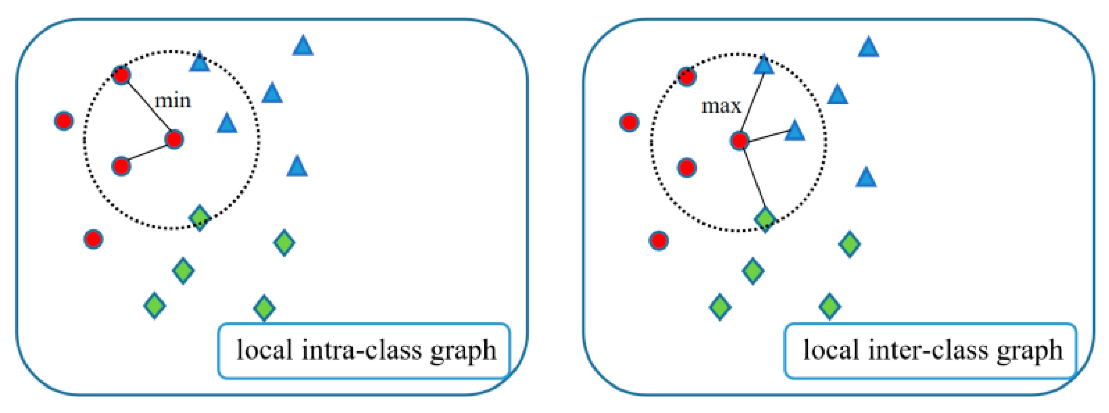
3.2. Construction of Local Objective Function

The local information reflects the neighborhood structure relationship between samples, and extracting effective neighborhood discriminant features is important to improve the accuracy of fault classification. For better classification, ESBDP expects samples belonging to the same class in the neighborhood to be more aggregated and samples in different classes to be separated from each other. Therefore, we combine the label information to construct local intra-class graph G l o c a l + and local inter-class graph G l o c a l . An example of graph construction is given in Figure 1.
G l o c a l + = ( X , W l o c a l + ) describes the structural relationships among the intra-class samples in the neighborhood, where X denotes the set of samples and W l o c a l + is the similarity matrix. W l o c a l + is defined as
W l o c a l + = 1 + exp ( x ^ i x ^ j 2 2 2 t 2 ) ,   i f   x ^ j N k ( x ^ i )   a n d   c ( x ^ i ) = c ( x ^ j ) 0 ,                           otherwise ,
where x ^ i denotes the Euler representation of x i , t is a kernel parameter and c ( x ^ i ) is the class of x ^ i .
According to Equation (10), the closer two sample points in the Euler space are, the greater the similarity between them. To maintain the structural relationship between the near-neighbor samples within the class after projection and obtain more compact intra-class local features, the local intra-class objective is defined as
G lcoal + = min P i , j = 1 n W l o c a l + P T x ^ i P T x ^ j 2                                                         = min   P P T X ^ D l c o a l + X ^ T P P T X ^ W l o c a l + X ^ T P ,                                                         = min   P P T X ^ L l o c a l + X ^ T P
where D l c o a l + is a diagonal matrix with diagonal elements equal to the column sum of W l o c a l + and L l o c a l + = D l c o a l + W l o c a l + is the Laplace matrix.
The local inter-class graph G l o c a l = ( X , W l o c a l ) is used to reflect the interclass structure of the data in the neighborhood, and its similarity matrix W l o c a l is constructed as
W l o c a l = 1 exp ( x ^ i x ^ j 2 2 2 t 2 ) ,   i f   x ^ j N k ( x ^ i )   a n d   c ( x ^ i ) c ( x ^ j ) 0 ,                           otherwise .
To improve the separability of local inter-class samples, the maximization objective function is defined as
G l o c a l = max P i , j = 1 n W l o c a l P T x ^ i P T x ^ j 2                                                           = max   P P T X ^ D l o c a l X ^ T P P T X ^ W l o c a l X ^ T P ,                                                           = max   P P T X ^ L l o c a l X ^ T P
where D l c o a l is a diagonal matrix, ( D l c o a l ) i i = j ( W l o c a l ) i j and L l c o a l = D l c o a l W l o c a l is the Laplace matrix. According to Equation (12), the smaller the distance between two near-neighbor sample points belonging to different classes in Euler space, the smaller similarity is assigned to them. By maximizing the objective function, the local inter-class features with more separation can be obtained.

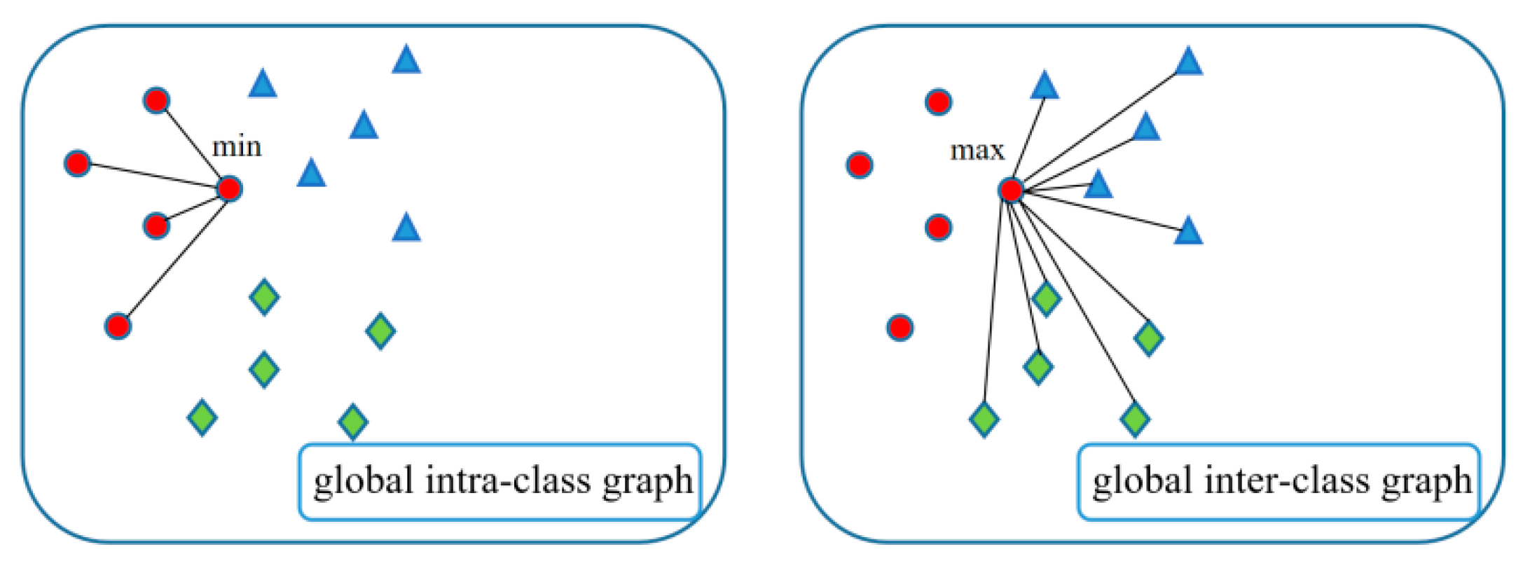
3.3. Construction of Global Objective Function

The global information can reflect the overall characteristics of the fault data, which is equally important for improving the fault diagnosis accuracy. To comprehensively explore the global information, we constructed a global intra-class graph G g l o b a l + = ( X , W g l o b a l + ) and a global inter-class graph G g l o c a l = ( X , W g l o c a l ) . An example of global graph construction is given in Figure 2.
G g l o b a l + reflects the geometric relationship between any two samples in the same class, and its similarity matrix W g l o b a l + is defined as
W g l o b a l + = x ^ i x ^ j 2 2 ( 1 + exp ( x ^ i x ^ j 2 2 2 t 2 ) ) ,   if   i j   and   c ( x ^ i ) = c ( x ^ i ) 0 ,                                                                 otherwise .
To make the fault data of the same class more aggregated after projection, the global intra-class objective is constructed as
G g l o b a l + = min P i , j = 1 n W g l o b a l i j P T x ^ i P T x ^ j 2                                                             = min   P P T X ^ D g l o b a l X ^ T P P T X ^ W g l o b a l X ^ T P ,                                                             = min   P P T X ^ L g l o b a l + X ^ T P
where D g l o b a l + is a diagonal matrix, ( D g l o b a l + ) i i = j ( W g l o b a l + ) i j and L g l o b a l + = D g l o b a l + W g l o b a l + is the Laplace matrix.
G g l o c a l reflects the geometric relationship between any two samples of different categories, and its similarity matrix W g l o b a l is defined as
W g l o b a l = x ^ i x ^ j 2 2 ( 1 exp ( x ^ i x ^ j 2 2 2 t 2 ) ) ,   if   i j   and   c ( x ^ i ) c ( x ^ i ) 0 ,                                                                 otherwise ,
The maximization global inter-class objective is defined as follows:
G g l o b a l = max P i , j = 1 n W g l o b a l P T x ^ i P T x ^ j 2                                                                 = max   P P T X ^ D g l o b a l X ^ T P P T X ^ W g l o b a l X ^ T P ,                                                                 = max   P P T X ^ L g l o b a l X ^ T P
where D g l o b a l is a diagonal matrix, ( D g l o b a l ) i i = j ( W g l o b a l ) i j and L g l o b a l = D g l o b a l W g l o b a l is the Laplace matrix. In Equation (16), two samples belonging to different classes in Eulerian space are approximately close to each other; then, a lower similarity is imposed between them, and under the incentive of maximization objective, the two samples in low-dimensional space move away from each other, thus obtaining global inter-class features with well separability.

3.4. The Uniform Object Function of ESBDP

Based on the above analysis, ESBDP expects to capture both local and global discriminative information of fault data in Euler space and make the data have better inter-class separability and intra-class aggregation after projection. Therefore, the objective function of ESBDP is formulated as four optimization problems:
min   P P T X ^ L l o c a l + X ^ T P max   P P T X ^ L l o c a l X ^ T P min   P P T X ^ L g l o b a l + X ^ T P max   P P T X ^ L g l o b a l X ^ T P .
To better unify the four objective functions into a single objective model, we transform the intra-class minimization problem into the equivalent maximization problem.
min   P P T X ^ L l o c a l + X ^ T P = P T X ^ ( D l o c a l + W l o c a l + ) X ^ T P             max   P P T X ^ W l o c a l + X ^ T P
min   P P T X ^ L g l o b a l + X ^ T P = P T X ^ ( D g l o b a l + W g l o b a l + ) X ^ T P             max   P P T X ^ W g l o b a l + X ^ T P
Combining the above four optimization problems, the objective model of ESBDP is defined as
max   P P T X ^ ( 1 δ ) ( L l o c a l + W l o c a l + ) + δ ( L g l o b a l + W g l o b a l + ) X ^ T P                                             s . t .   P T X ^ ( D l o c a l D g l o b a l ) X ^ T P = 1 .
where D l o c a l = D l o c a l + + D l o c a l , D l o c a l = D g l o b a l + + D g l o b a l and δ [ 0 , 1 ] is a balance parameter to regulate the elasticity between global and local information.
In Equation (21), the balance parameter determines the relative importance of the global and local targets, which plays an essential role in obtaining effective fault features. However, there are some problems that need to be solved here, such as the determination of the appropriate parameter values. Usually, the parameter needs to be set artificially in the range first, and the final parameter value is obtained by methods such as grid search. It is a challenge to manually select a suitable parameter in different fault applications, and the discriminative power of the extracted relevant features may reduce if the parameter is not selected properly. Therefore, we offer an adaptive balancing strategy to further optimize the uniform objective function of ESBDP.

3.5. Optimization of the Uniform Objective Function

In this section, we offer an adaptive balance strategy to construct an optimized model for ESBDP. Compared with setting the parameters manually, we expect the ESBDP algorithm to adaptively select the best balancing parameters to achieve an effective balance of global and local features, thus further enhancing the discriminative power of the extracted fault features. Therefore, Equation (21) is optimized as follows:
arg max   P , α l , α g α l 2 P T X ^ H l o c a l X ^ T P + α g 2 P T X ^ H g l o b a l X ^ T P                                     s . t .   P T X ^ ( D l o c a l D g l o b a l ) X ^ T P = 1 .                                     , α l + α g = 1 .
where H l o c a l = L l o c a l + W l o c a l + , H g l o b a l = L g l o b a l + W g l o b a l + , α l corresponds to the weight parameter of the local target and α g is the weight parameter of the global target. While learning the local and global structural features of the fault data, the model of Equation (22) obtains intra-class minimization and inter-class maximization, and in addition, the model achieves adaptive balance between global and local objectives.
In the optimization model of ESBDP, the projection direction and the balance parameters are the objectives to be solved. Since it is difficult to solve both objectives at the same time, we use a way of iterative update, i.e., fix one solution objective, update the other one, and stop the iterative process when the solution converges. The following are the solution steps.
(1) Fixing the balance parameters α l and α g , we update the projection matrix P .
Fixing the balance parameters as constants, Equation (22) can be expressed as
arg max   P α l 2 P T X H l o c a l X T P + α g 2 P T X H g l o b a l X T P         s . t .   P T X ( D l o c a l D g l o b a l ) X T P = 1 .
The Lagrange multiplier method was used to solve for Equation (23).
L ( P ) = α l 2 P T X H l c o a l X T P + P T X α g 2 H g l o b a l X T P λ ( P T X ( D l o c a l D g l o b a l ) X T P 1 )
where λ is the Lagrangian multiplier. The value of the partial derivative of Equation (24) with respect to P is zero.
L ( P ) P = α l 2 X H l o c a l X T P + α g 2 X H g l o b a l X T P λ X ( D l o c a l D g l o b a l ) X T P 1 = 0 .
Then, Equation (25) can be transformed into
α l 2 X H l c o a l X T P + α g 2 X H g l o b a l X T P = λ X ( D l o c a l D g l o b a l ) X T P .
Solving Equation (26), we can calculate that the eigenvector λ = [ λ 1 , λ 2 , , λ d ] corresponds to the first d largest eigenvalues, which is the desired projection direction.
(2) Fixing P , we update α l and α g .
Fixing the projection matrix, Equation (18) can be expressed as
arg max   α l , α g α l 2 P T X H l o c a l X T P + α g 2 P T X H g l o b a l X T P s . t .   α l + α g = 1 .
Using the Lagrange multiplier method to solve Equation (27).
L ( α l , α g ) = α l 2 t r ( P T X H l o c a l X T P ) + α g 2 t r ( P T X H g l o b a l X T P ) λ ( α l + α g 1 ) .
We let the value of the partial derivative of Equation (28) with respect to the balance parameter be zero.
L ( α l , α g ) α l = 2 α l t r ( P T X H l o c a l X T P ) λ = 0 L ( α l , α g ) α g = 2 α g t r ( P T X H g l o b a l X T P ) λ = 0 L ( α l , α g ) λ = α l + α g 1 = 0 .
By mathematical transformation, the balance parameters can be expressed as
α l = t r ( P T X H g l o b a l X T P ) t r ( P T X H l o c a l X T P ) + t r ( P T X H g l o b a l X T P ) ,
α g = t r ( P T X H l o c a l X T P ) t r ( P T X H l o c a l X T P ) + t r ( P T X H g l o b a l X T P ) .
Finally, the fault data are projected into the subspace by Y = P T X to obtain the low-dimensional representation features. Algorithm 1 describes the steps of the ESBDP algorithm.
Algorithm 1 Euler Representation Based Structural Balance Discriminant Projection
Input: Training fault sample set X [ x 1 , x 2 , , x n ] R m × n
Output: projection matrix P
(1) Conversion of the original feature data X into Euler representation data X ^ by Equation (9).
(2) Construction the weight matrix W l o c a l + , W l o c a l + , W g l o b a l + and W g l o b a l .
(3) Fixing the balance parameters α l and α g , update P .
(4) Fixing the projection matrices P , update α l and α g .
(5) Repeat (3) and (4) until convergence.

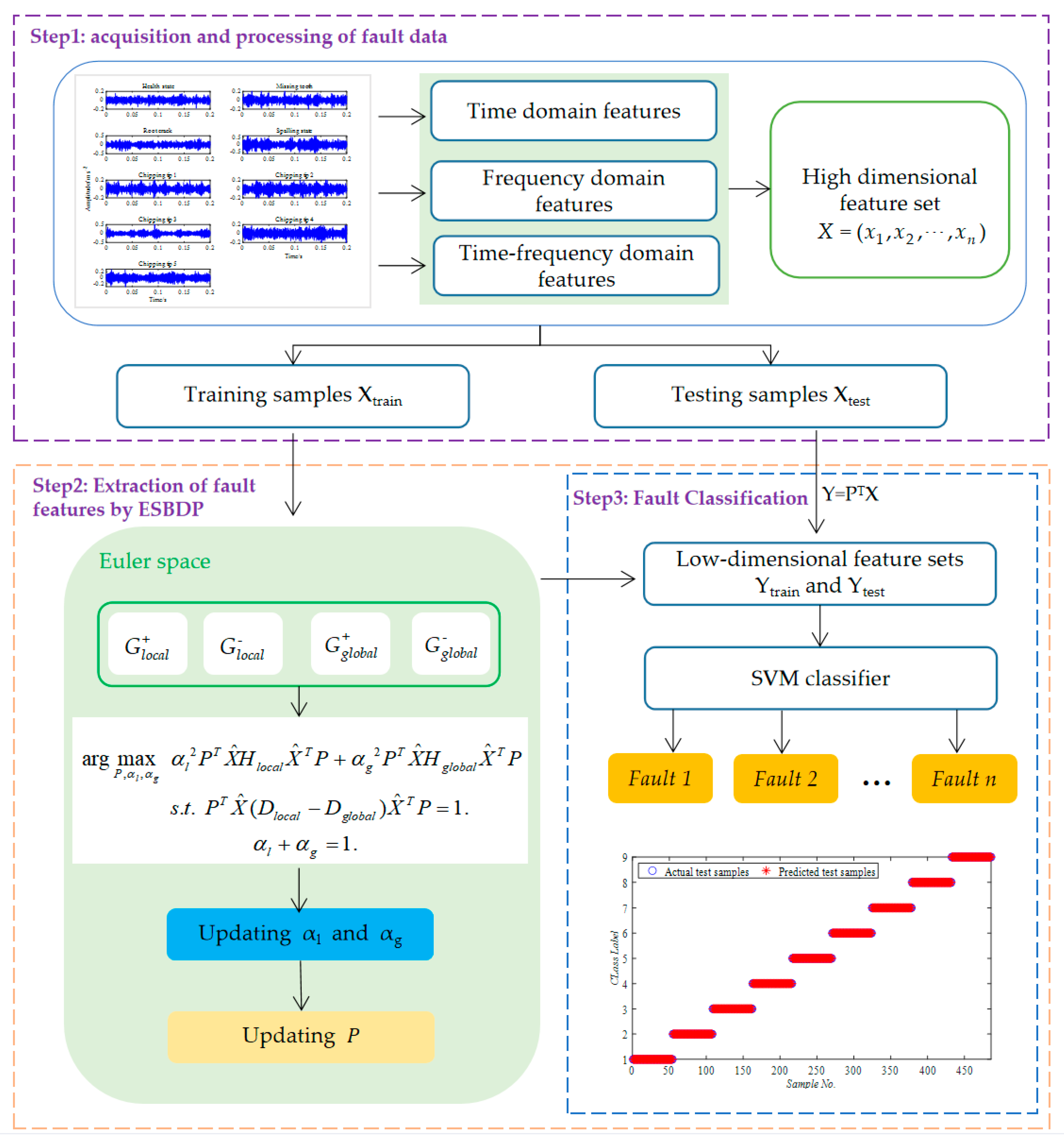
4. Fault Diagnosis Process Based on ESBDP Algorithm

In this section, the fault diagnosis process based on the ESBDP algorithm is described, and the diagnosis flowchart is provided in Figure 3, where n denotes the number of classes of fault data. The following is a specific description of the diagnosis steps:
Step 1. The vibration data of machinery equipment during operation are collected, and the original data are transformed into time–frequency domain features to construct a high-dimensional fault feature set. The high-dimensional feature set can reduce the influence of the noise and the nonlinear features in the original data [43]. The relevant characteristic parameters are provided in Table 2, where v ( i ) denotes the time series of the signal and s ( k ) is the frequency spectrum of v ( i ) . In Table 3, p1~p17 are the time domain features, which are mean value, square root amplitude, peak value, absolute mean, maximum value, root mean square value, variance, minimum value, standard deviation, impulse factor, kurtosis, skewness, waveform factor, peak factor, peak-to-peak value, margin factor and gap factor. p18~p21 are the frequency domain features of the signal, which are the mean frequency, center of gravity frequency, root mean square frequency, and standard deviation of frequency. p22~p29 are the time–frequency domain features of the signal. More specific definitions of the feature parameters can be referred to [9,10,28,44]. Then, the feature set is divided into a training set X t r a i n and a testing set X t e s t in a certain proportion by means of a random selection.
Step 2. The training set X t r a i n is mapped to the Euler space, and the ESBDP optimization model based on four objectives is constructed in this space. Solving this model, we can obtain the projection matrix P. Then, the low-dimensional representation features Y t r a i n and Y t e s t are obtained by projecting X t r a i n and X t e s t into the subspace using P .
Step 3. The low-dimensional training sample Y t r a i n is input to the SVM classifier for learning, and finally, the fault type of the test sample is predicted based on the completed training classifier.

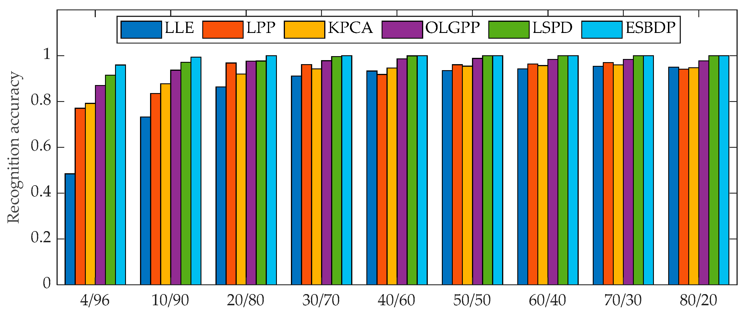
5. Experimental Results and Analysis

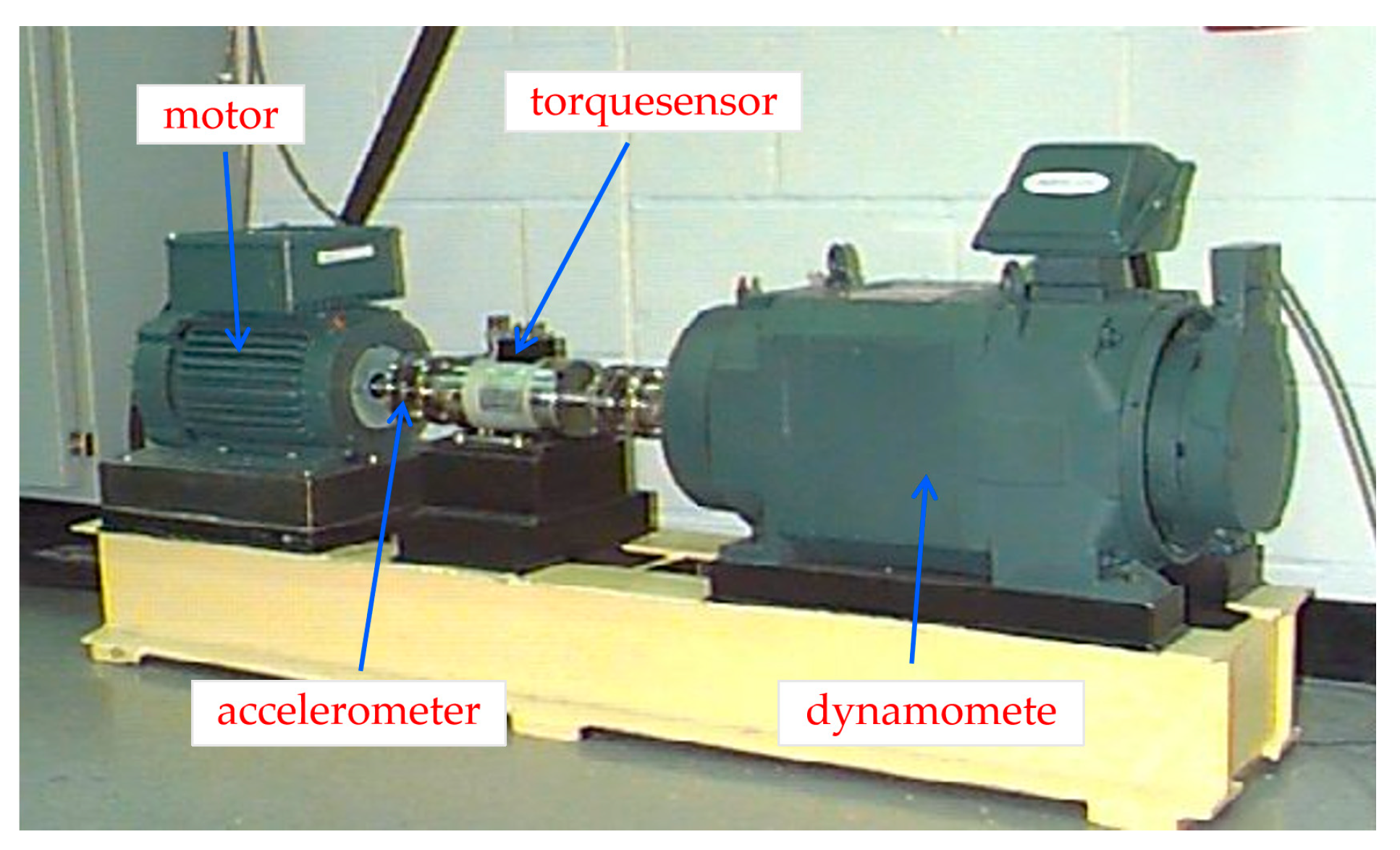
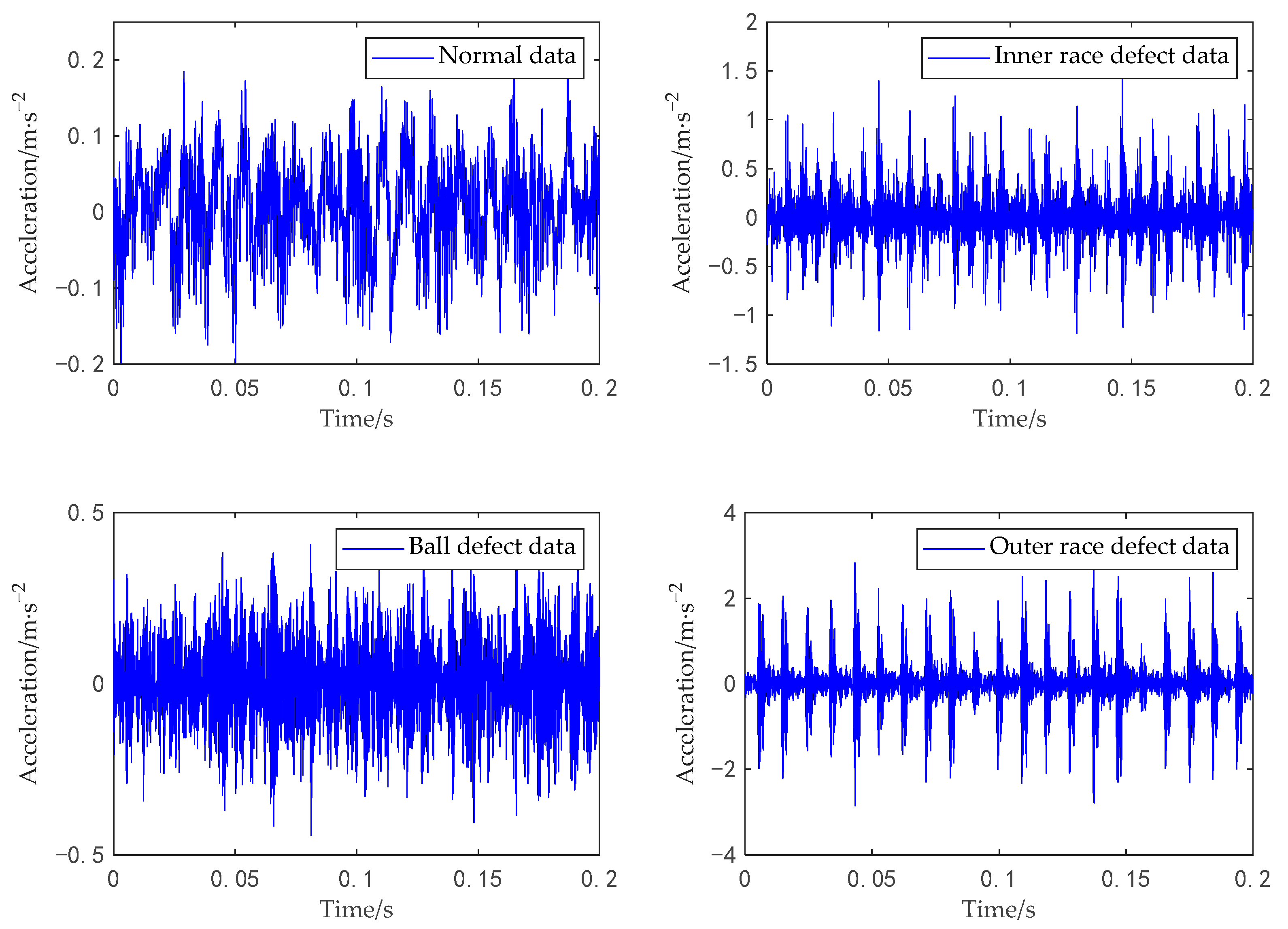
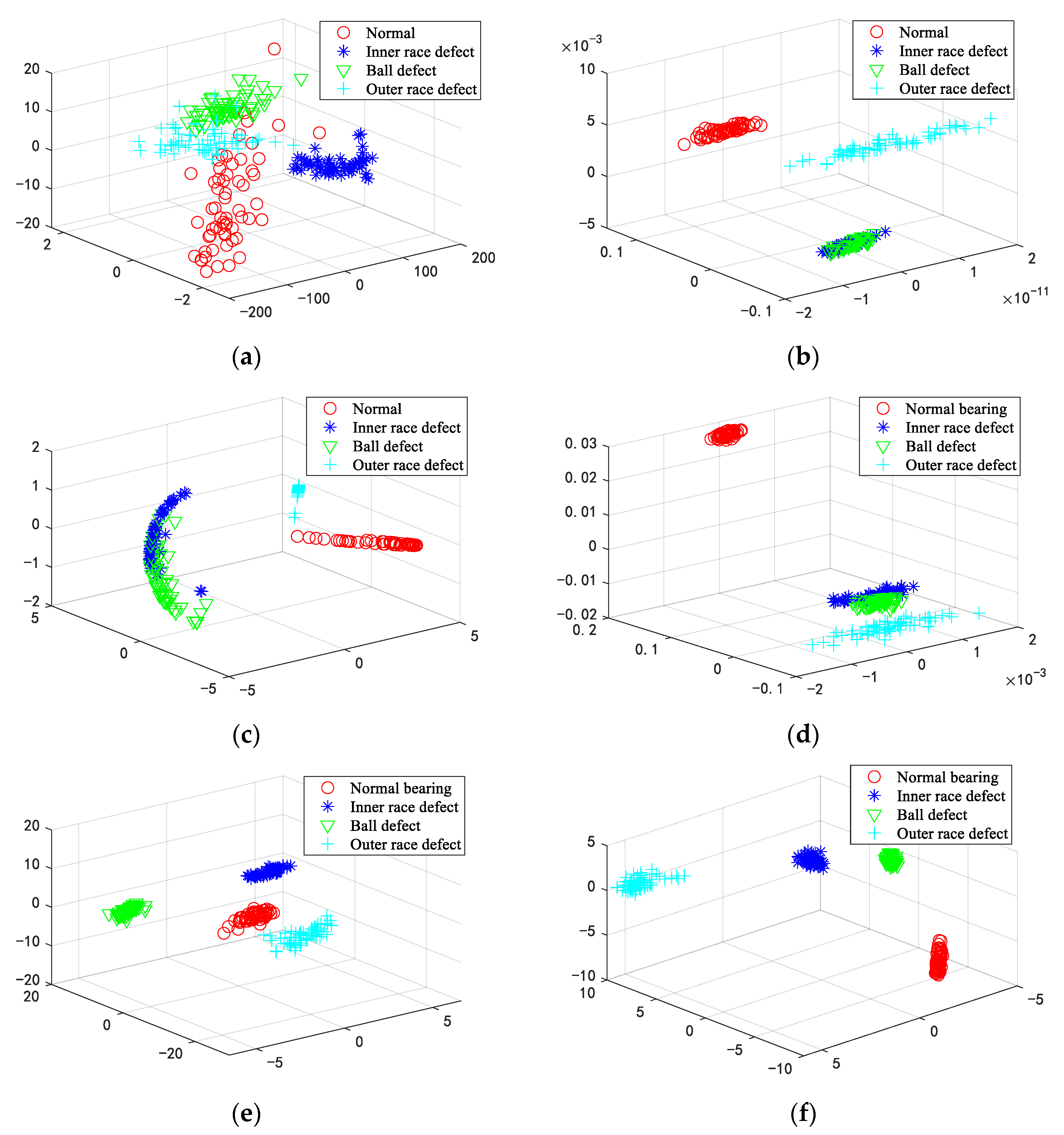
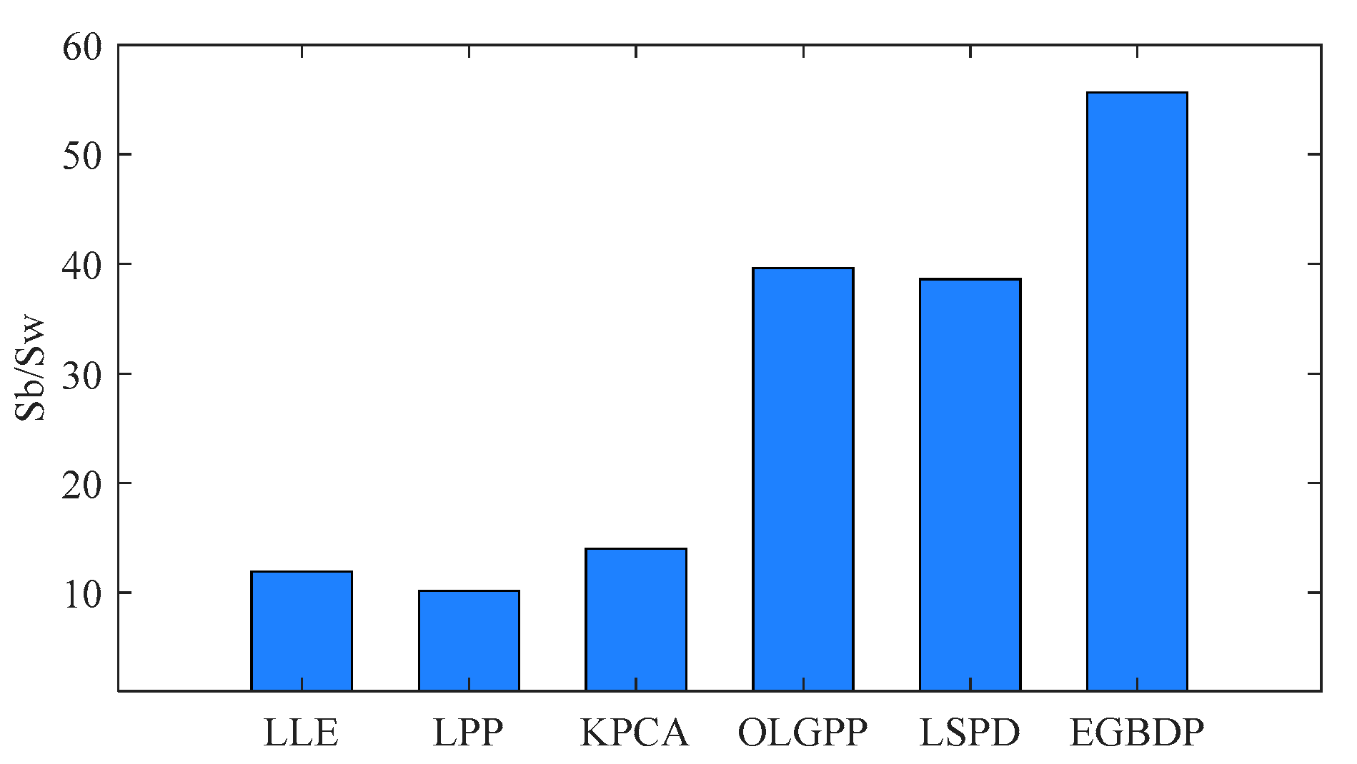
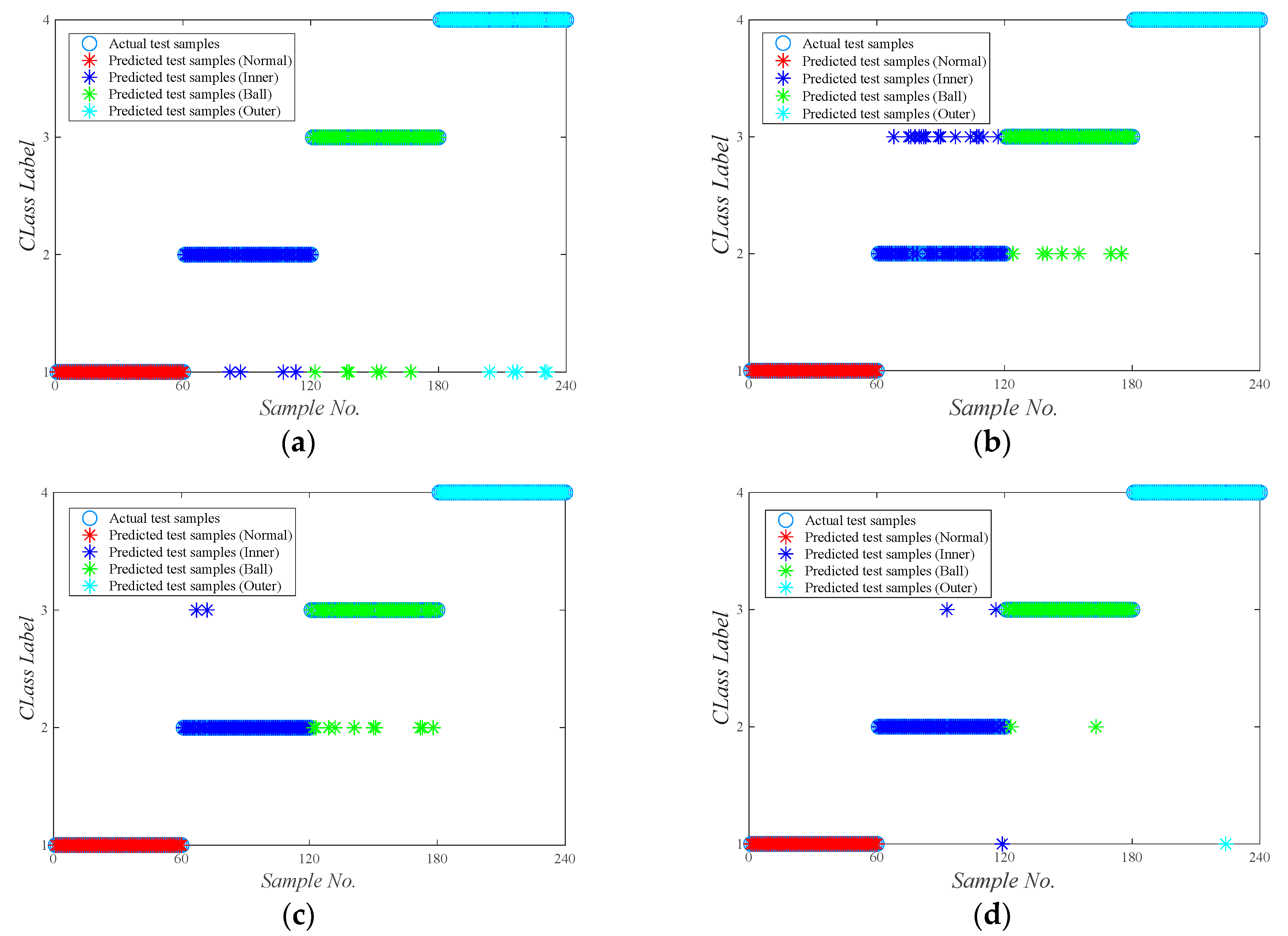
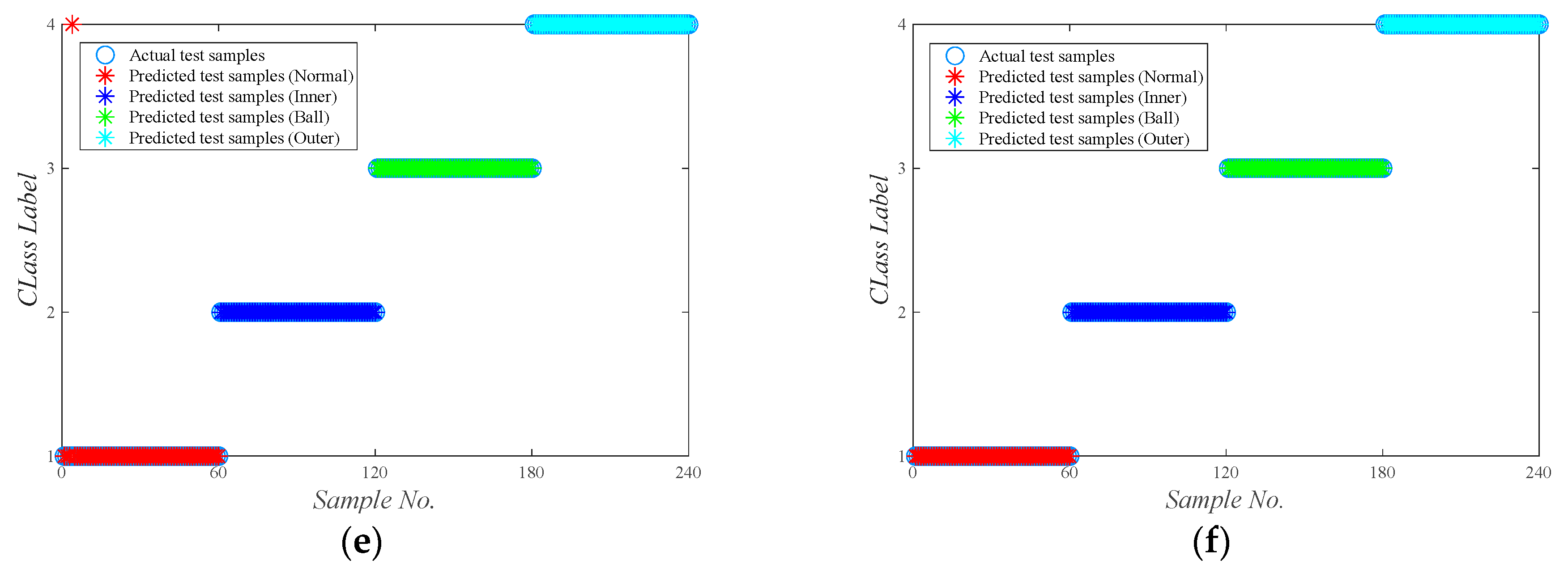
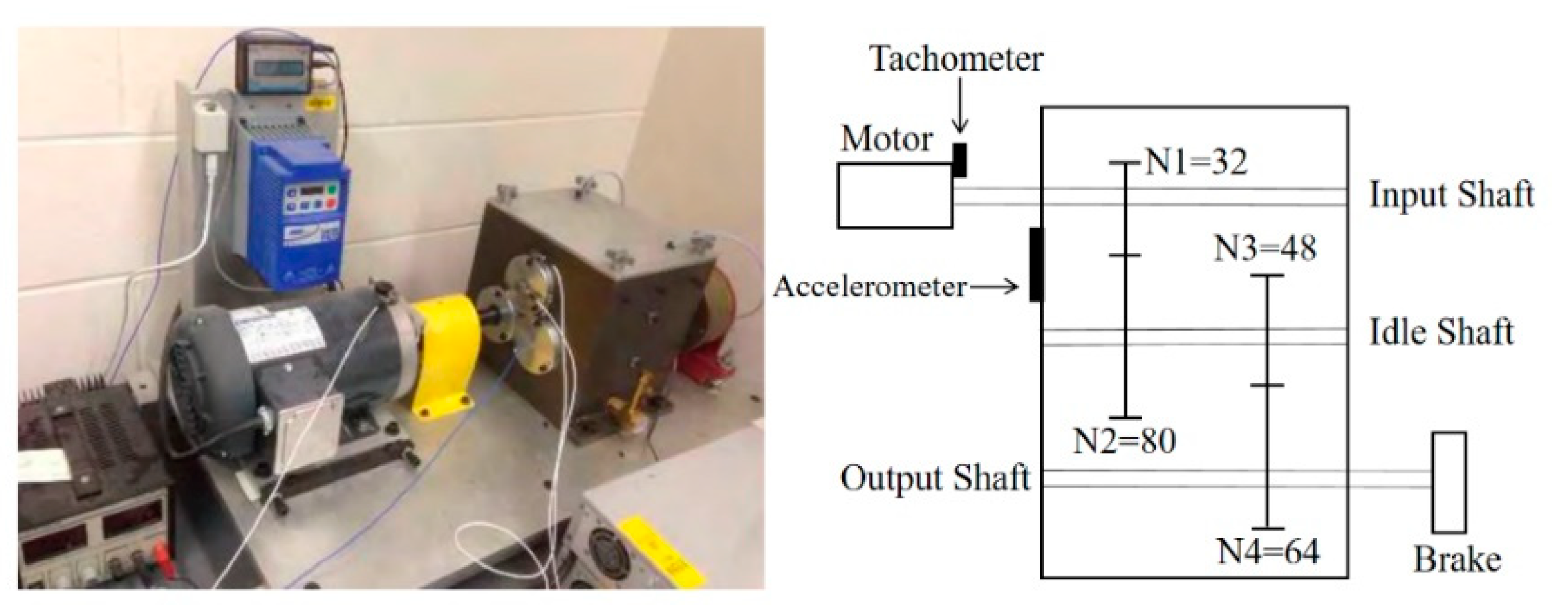
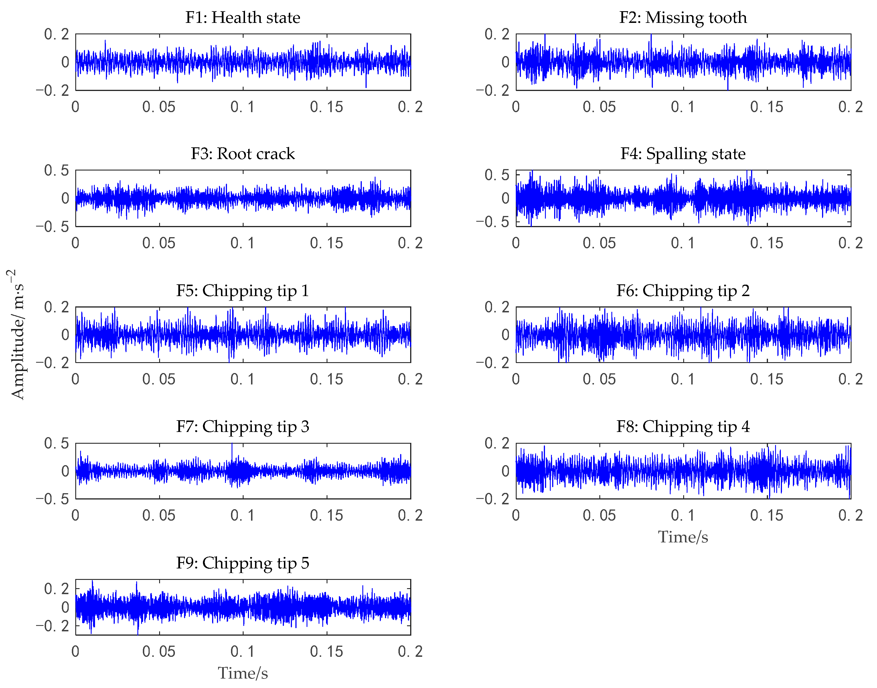
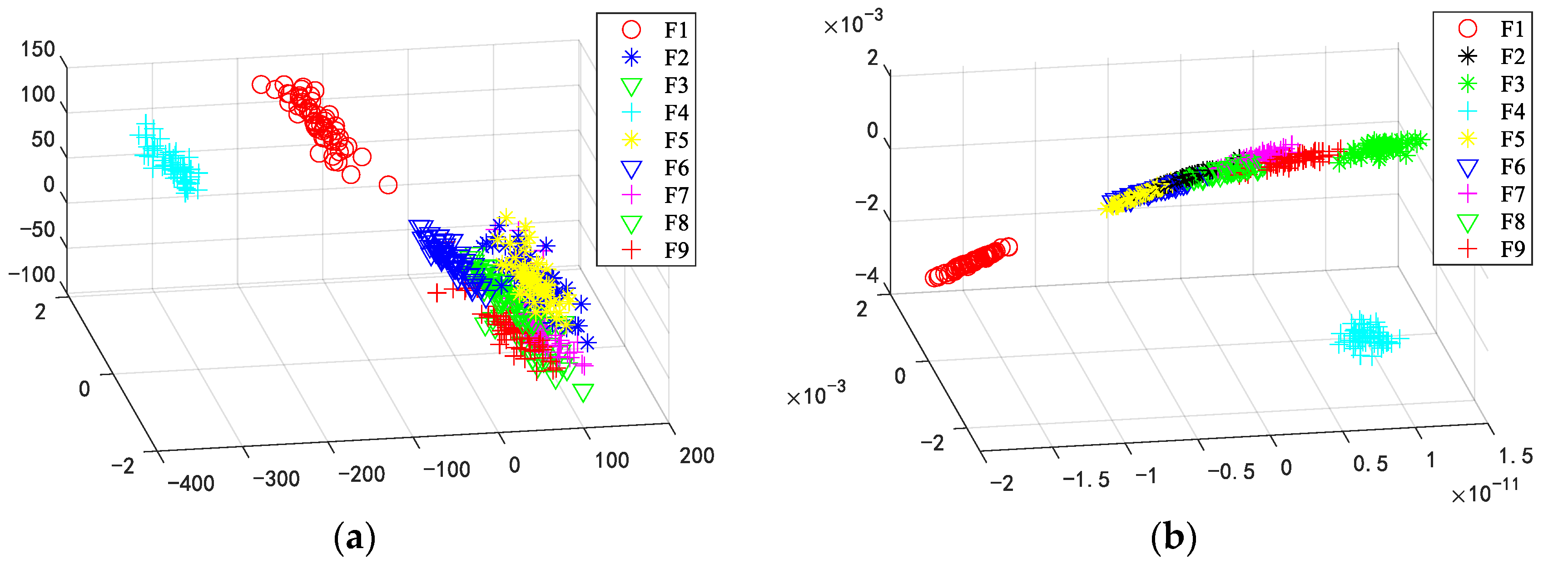
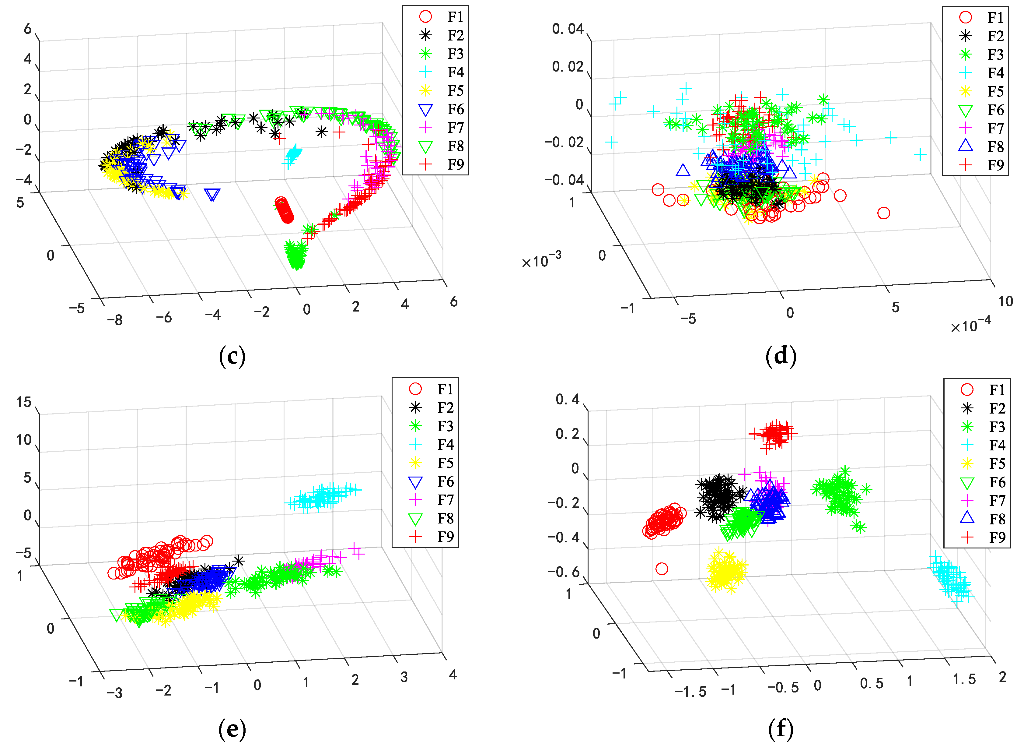
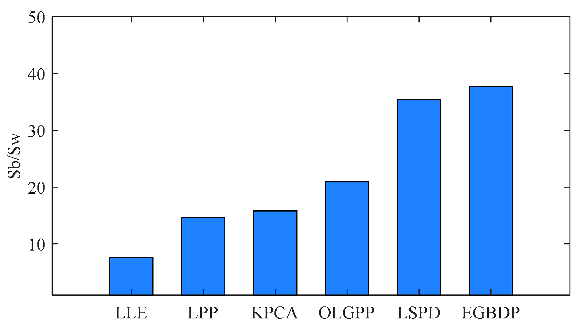
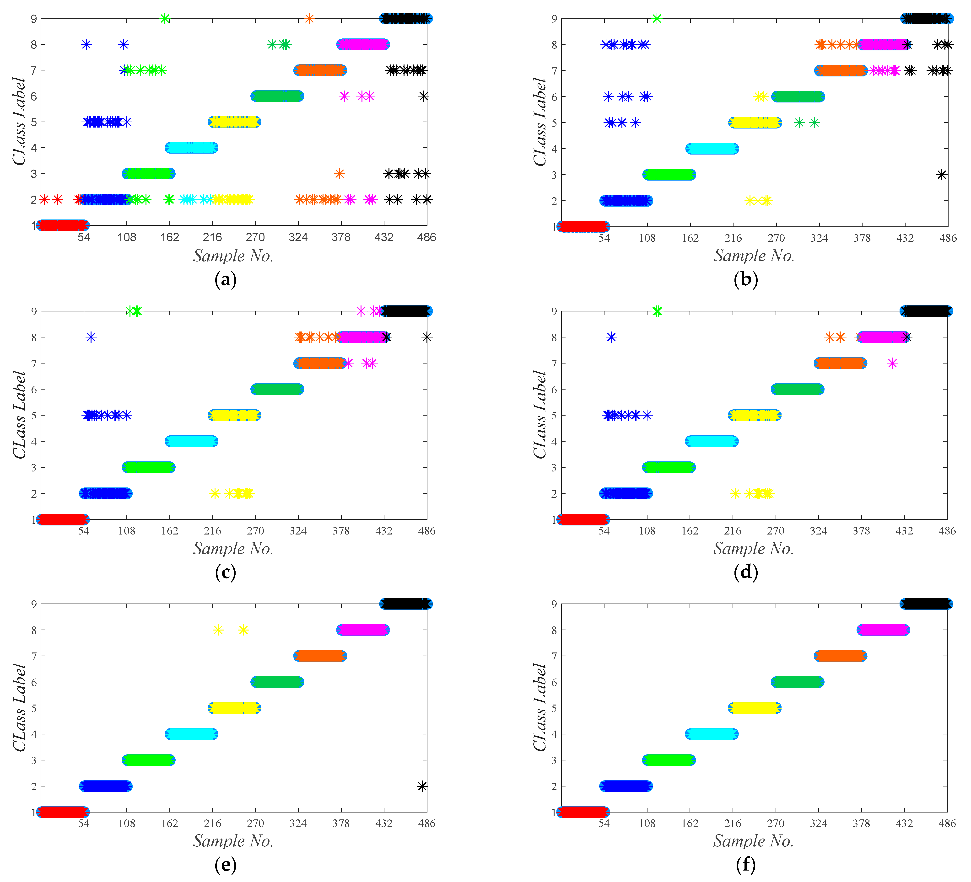
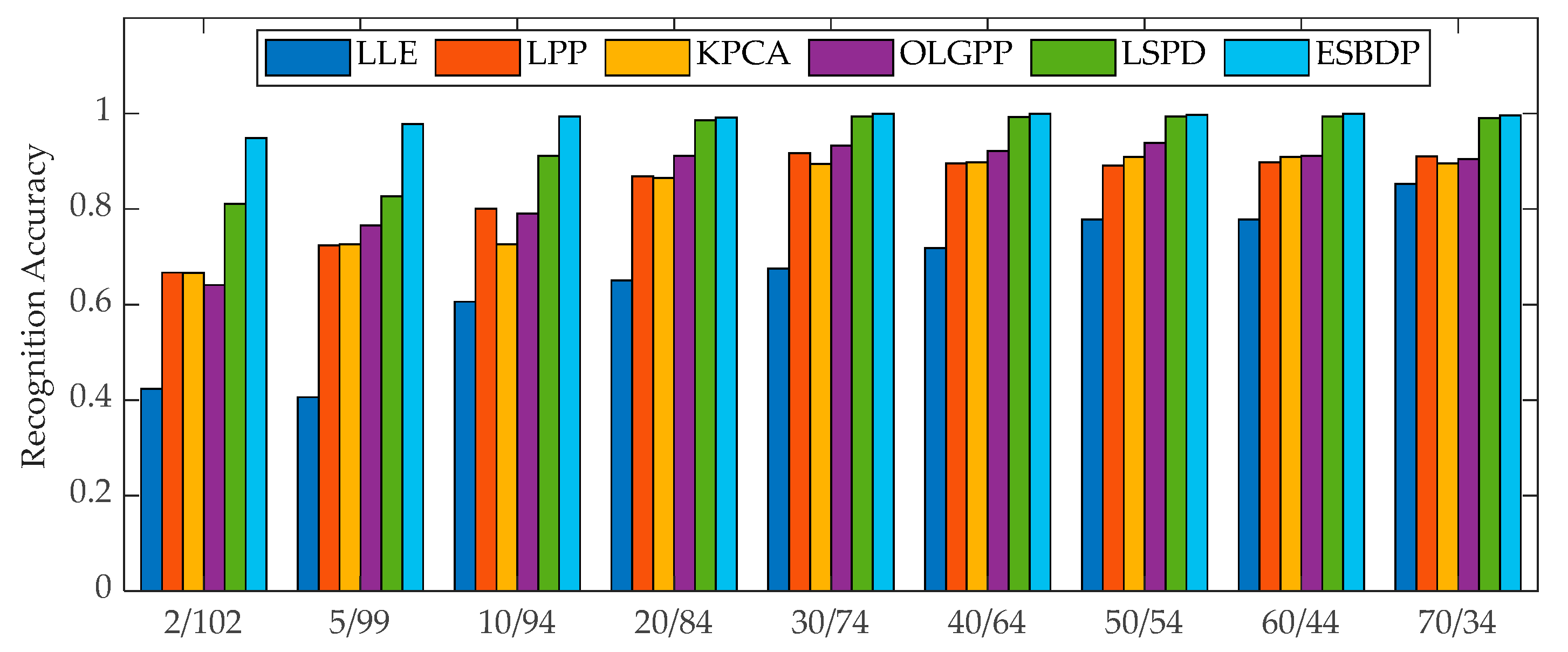
5.1. Experiments on the Bearing Dataset

In this experiment, the bearing data were used from the Case Western Reserve University (CWRU) rolling bearing dataset. As shown in Figure 4, the data acquisition platform is divided into three main parts, from left to right, the motor, the torque sensor, and the dynamometer. The drive-end bearing vibration data at 12 kHz sampling frequency and 1772 rpm were used in our diagnosis experiment, containing four different types of data, namely normal data, inner race defect data, outer race defect data and ball defect data. Figure 5 shows the one-dimensional signals of the four states. With a sampling length of 1024, 100 samples were obtained for each type of signal data. Then, the high-dimensional feature set is obtained by extracting the time–domain, frequency–domain and time–frequency features of the original fault samples according to the process described in Section 4. The training set is composed of 40 samples randomly selected from each class, and the rest are used as test samples. To avoid the chance of experimental results, the random experiment was repeated ten times by us. Finally, the fault recognition accuracy was taken as the average of the ten-time results.
To obtain the appropriate parameters for the ESBDP algorithm, we conducted several experiments using the grid search method, and through comparison, we finally set the neighborhood parameter value k = 9 , the adjustment parameter γ = 1 , and the kernel parameter t = 0.01 . In addition, for comparison with our algorithm, five related algorithms, KPCA, LPP, LLE, OLGPP, and LSPD were used for the same experiments, and the parameters of each algorithm were selected using the grid search method. Among them, the kernel parameter of the global nonlinear algorithm KPCA is t k p c a = 2 . The neighborhood parameters of the LPP, LLE, OLGPP, and LSPD [45] algorithms are set to k l p p = 12 , k l l e = 7 , k olgpp = 17 , and k lspd = 10 , respectively. The kernel parameters of LPP, KPCA and OLGPP are set to t l p p = 1 and t olgpp = 0.1 , respectively.
To visualize the classification performance of ESBDP, we show the distribution of the sample features in the three-dimensional space after projection in Figure 6 and compare it with the LLE, LPP, KPCA, OLGPP and LSPD algorithms, where the horizontal axis denotes the first dimension of Y t e s t , the vertical axis denotes the second dimension of Y t e s t , and the other axis denotes the third dimension of Y t e s t . It can be seen that the visualization distribution results of LLE, LPP and KPCA are relatively poor, showing that the same kind of features are scattered and there is a serious overlap between different types of data without a clear demarcation. The reason for this situation is that all three algorithms only singularly consider the neighborhood information or global structure of the fault data and extract incomplete information; in addition, the supervision information is not used by these algorithms. Compared with the above three algorithms, the visualization results of OLGPP and LSPD are relatively good, but there are some cases of scattered data within the class and the heterogeneous samples are relatively close to each other. The visualization of the three-dimensional feature distribution based on the ESBDP method is optimal, with high aggregation between the same class of samples, high separation between the heterogeneous samples, and obvious demarcation between classes, which provides a favorable basis for the subsequent fault classification.
To further explain the low-dimensional feature separability of ESBDP, we adopted the ratio of inter-class distance and intra-class distance as the separability index. The inter-class distance S b is used to reflect the separability between classes, while the intraclass distance S w reflects the aggregation of samples within classes, and they can be calculated by Equations (32) and (33), where c denotes the number of classes of samples, y ¯ i = i = 1 n y i / n denotes the class center, and y j i denotes the i th sample of the j th class. For low-dimensional features, the larger the separability parameter metric, the better its relative separability. Figure 7 provides the divisibility metrics based on the six algorithms, and it can be seen that the divisibility parameters of EGBDP are higher than those of the other algorithms. Combining Figure 6 and Figure 7, we can conclude that ESBDP has better dimensionality reduction performance and can provide a favorable basis for subsequent fault classification.
S b = 1 c ( c 1 ) i , j c y ¯ i y ¯ j ,
S w = 1 c j = 1 c 1 n i n y j i y ¯ j
Table 3 provides the average fault recognition accuracy and its standard deviation and processing time for ten random experiments based on the six methods of LLE, LPP, KPCA, OLGPP, LSPD and ESBDP. The standard deviation is used to reflect the fluctuation of the recognition rate such as the smaller standard deviation indicating the smoother performance of the algorithm. From Table 3, it can be observed that the recognition results of the three algorithms, LLE, LPP and KPCA, which only consider the global or local structure, are lower for nonlinear unstable machinery fault data. Among them, LPP has a recognition rate of 91.79% by discovering the local discriminative features on the sample manifold, and the large standard deviation indicates its poor stability. LLE is a nonlinear algorithm in the manifold algorithm that can respond to the sample globally with local linearity, and its low-dimensional samples can keep the original topology, and the fault diagnosis accuracy of this algorithm is 93.29%. With the kernel function, KPCA can capture the nonlinear global structure information of the fault data, and the recognition rate is 94.63%. Since OLGPP captures both global and local information of the data, its diagnosis accuracy is higher than the above three methods, but OLGPP does not utilize the supervised information of the fault data, so it is difficult to achieve the correct classification of all the data. While using supervised information, LSPD measures and preserves the similarity between fault samples by constructing a similarity function, which improves the accuracy to some extent, but the algorithm focuses more on the local structure of the samples and the global information is not effectively used.
ESBDP achieves the highest recognition accuracy because the algorithm maps the fault data into the Euler space through the cosine metric and integrates the structural relationships of local intra-class, local inter-class, global intra-class and global inter-class samples in this space. On the basis of expanding the differences between heterogeneous fault samples, the inter-class separation and intra-class aggregation between samples are effectively improved. In addition, ESBDP achieves an adaptive balance between global and local features, which further enhances the discriminative power of the extracted fault features. Remarkably, our method has the smallest standard deviation and the processing time is only 0.34 s, which means that the ESBDP algorithm has a low computational burden and is more stable.
The specific classification results are provided in Figure 8. It can be observed that the classification errors exist in all algorithms except our algorithm. Among them, in the prediction results of the LPP and KPCA algorithms, the classification errors are mainly concentrated on the second and third fault types of data. Classification errors are detected in LLE and OLGPP for all other three types of faults except normal data. The classification results of the LSPD algorithm are better, but there is also a normal sample that is misclassified. Our method can accurately identify samples of each fault type, which shows the superiority of ESBDP in clustering and classification of all types of fault data.
To further verify the ability of the ESBDP algorithm to capture fault information, we used different numbers of samples to train each algorithm and then observed the change in fault diagnosis results. Figure 9 shows the corresponding experimental results. Overall, as the number of training samples increases, the recognition rate of all six algorithms increases, because the training samples contain the discriminative information required for fault classification, and the more training samples, the more discriminative features can be learned. Among them, LLE, LPP and KPCA algorithms have lower recognition rates. In addition, the accuracy of LPP, LLE and KPCA can hardly be improved even if the training samples are increased due to the performance of the algorithms. ESBDP outperforms the other five algorithms in terms of recognition rate and stability. It is worth noting that ESBDP can achieve a 100% fault recognition rate at 20 training samples per class, which means that our algorithm has a strong ability to capture fault discriminative information and can better perform fault diagnosis tasks.
To further investigate the performance of the ESBDP algorithm, we experimented with bearing fault data for four operating conditions at 1797 r/min, 1772 r/min, 1750 r/min, and 1730 r/min, respectively. Following the process in Chapter 3, the identification results of the six algorithms are shown in Figure 10. It can be concluded that for the bearing data under different working conditions, the recognition rates of the first three algorithms are generally low and unstable, and the accuracy rates of OLGPP and LSPD are relatively good, but they cannot classify the four data correctly at the same time. The ESBDP algorithm is the most stable and achieves the highest accuracy rate for the diagnosis of all four data. Experiments show that compared with other methods, ESBDP has stronger adaptability and can also mine effective fault discrimination features for data under different working conditions to achieve accurate classification.

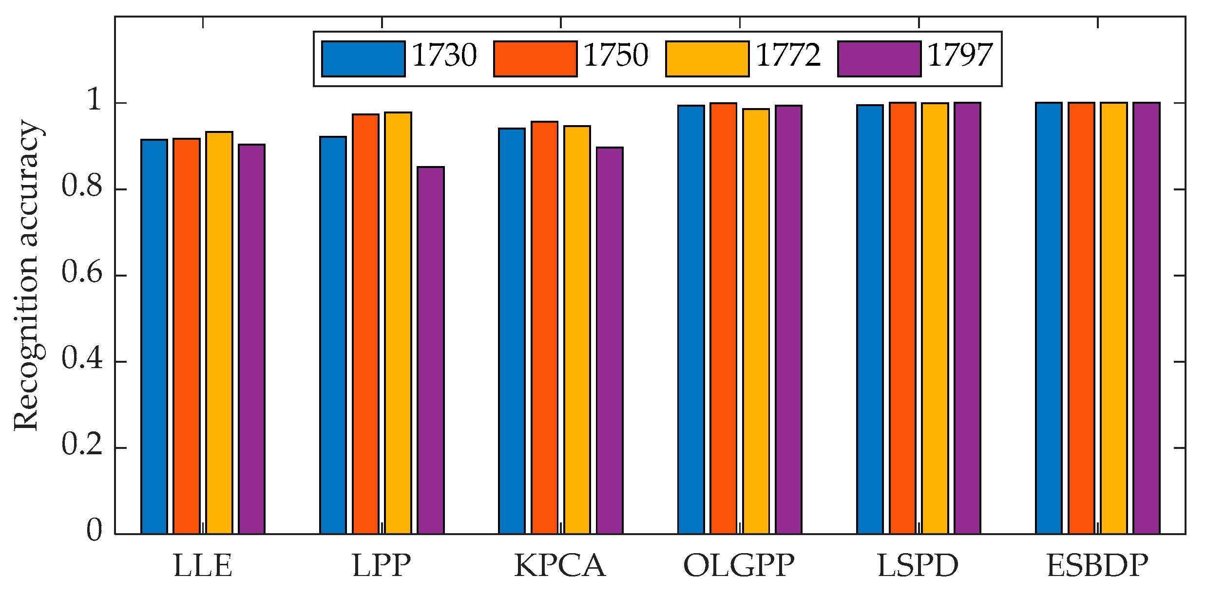
5.2. Experiments on the Gear Dataset

The experimental data were obtained from a gear fault dataset published by the University of Connecticut, and the data collection platform is shown in Figure 11. It is a two-stage gearbox containing a motor for controlling the gear speed, a tachometer for measuring the speed, an electromagnetic brake for providing torque, and two-stage input shaft equipped with gears. The gear operation data are obtained from the pinion of the first stage via an accelerometer with a sampling frequency of 20 KHZ and contain nine types of gear states for spalling, root crack, missing tooth, five different severity levels of chipping tip, and health state. To facilitate the description, we denote these nine types of data by {F1, F2, F3, F4, F5, F6, F7, F8, F9}. The vibration signals of the nine gear states are provided in Figure 12. A total of 104 samples were collected for each type of data, totaling 936 samples with a dimension of 3600. Following the procedure in Section 4, the statistical features in the time–frequency domain were computed for each sample to obtain the high-dimensional feature set. In this experiment, we randomly chose 50 samples from each of the nine data types as training samples and the rest of the samples as prediction samples. In addition, the parameters of each algorithm in the gear experiment are the same as those of the bearing diagnosis experiment.
Figure 13 and Figure 14 show the three-dimensional distribution and separability indexes of the low-dimensional features after projection based on the six algorithms, respectively. Due to the increase in categories, the distribution of features is more complex. Among them, the separable indexes of LLE, LPP and KPCA are relatively low and the visualization effect is relatively poor. There is a serious overlap between multi-category features without clear demarcation, which makes it difficult to identify effectively. The main reason is that these three methods only consider the neighborhood structure or global information of the fault data. OLGPP is also more confounded between classes because it does not utilize the label information between samples. The comparison shows that for multi-class gear fault data, the ESBDP method has the highest separability index and its three-dimensional feature distribution visualization is also optimal, where homogeneous features are aggregated with each other and heterogeneous features have relatively obvious boundaries, which shows that our algorithm can effectively improve the aggregation between samples of the same class and the separability between heterogeneous samples.
The gear diagnosis accuracy is provided in Table 4, and its corresponding classification details are provided in Figure 15. For gear data with multiple classes, the recognition accuracy of LLE, LPP and KPCA algorithms, which fail to combine both local and global discriminative features of fault data, decreases more. The accuracy of the OLGPP algorithm also decreases because the supervised information is not utilized by the algorithm, which makes it not advantageous in the diagnosis of multi-category fault data. In addition, there are more parameters in the OLGPP algorithm, which makes it hard to effectively diagnose different fault data without changing the parameters. It is worth noting that our algorithm achieves accurate classification for all types of gear data. On the basis of expanding the differences between heterogeneous samples, ESBDP combines label information to fully consider the geometric structure relationship of fault data to achieve the acquisition and balance of local and global features, which enables effective fault discriminative features to be extracted. The results of gear diagnosis further demonstrate the effectiveness of our algorithm.
To further verify the ability of ESBDP to capture fault features, the number of samples used for training and the number of samples used for prediction were set to 2/102, 5/99, 10/94, 20/84, 30/74, 40/64, 50/54, 60/44, and 70/34 in the gear diagnosis experiments, respectively, to observe the variation of the accuracy rate of each algorithm. The results are provided in Figure 16. For different numbers of training samples, the fault diagnosis accuracy of ESBDP is consistently higher than that of the other five algorithms. Notably, the recognition accuracy of ESBDP reaches 99.53% at 10 training samples per class, which indicates that the algorithm has a great ability to capture the discriminative features hidden in the fault data.

6. Conclusions

To address the problem of fault diagnosis methods sensitive to outliers and the difficulty to obtain and balance global and local discriminative information simultaneously, this paper proposes the ESBDP algorithm for rotating machinery fault diagnosis.
(1) The algorithm maps the high-dimensional fault features to the Euler representation space through the cosine metric, and the Euler representation approximates an ideal robust kernel that can suppress the influence of outliers in fault data. Meanwhile, the comparative analysis of Euler distance and Euclidean distance concludes that the heterogeneous fault samples have greater differences in the Euler space, which improves the inter-class separability to a certain extent.
(2) Through the adaptive balance strategy, the algorithm fully considers the geometric structure relationship of the fault data and constructs an optimization model based on four objective functions with different structure and class information in the Euler space, which can balance the local and global structures of the fault data and further im-prove the local intra-class aggregation and global inter-class separability of the low-dimensional discriminant features.
(3) In two rotating machinery fault experiments of bearings and gearboxes, the effectiveness and stability of the algorithm are analyzed from the perspectives of three-dimensional feature distribution of test samples, confusion matrix and fault recognition rate under multiple working conditions. The experimental results show that the algorithm proposed in this paper can effectively improve the accuracy of fault classification and has superior fault diagnosis performance.
Although ESBDP has many advantages, there are still some potential problems. For example, some parameter tuning is needed in the ESBDP algorithm, as well as a way to select parameter values adaptively. The selection of time and frequency domain feature parameters also affects the results of fault diagnosis and ways to obtain the optimal combination of time and frequency statistical features. All these issues will be further investigated in the future.

Author Contributions

Conceptualization, M.Z.; methodology, M.Z.; software, M.Z.; validation, M.Z., S.S. and Y.Z.; formal analysis, S.S.; investigation, T.W.; resources, S.S.; data curation, T.W.; writing—original draft preparation, M.Z.; writing—review and editing, S.S.; visualization, M.Z.; supervision, S.S.; project administration, M.Z. and S.S.; funding acquisition, M.Z., S.S. and X.F. All authors have read and agreed to the published version of the manuscript.

Funding

This research was funded by the Graduate innovation fund project of Anhui University of science and technology (Grant No. 2021CX2104), the Natural Science Research Project of Colleges and Universities in Anhui Province (Grant No. 2022AH040113), the University Synergy Innovation Program of Anhui Province (Grant No. GXXT-2021-006), the Postdoctoral Science Foundation of China (Grant No. 2019M660149), and the National Natural Science Foundation of China (Grant No. 61806006).

Institutional Review Board Statement

Not applicable.

Informed Consent Statement

Not applicable.

Data Availability Statement

Data presented in this study are available in this article.

Acknowledgments

We would like to thank the Case Western Reserve University (CWRU) Bearings Data Center and Jiong Tang’s team at the University of Connecticut for providing the dataset.

Conflicts of Interest

The authors declare no conflict of interest.

Abbreviations

PCAprincipal components analysis
KPCAkernel principal components analysis
LLElocal linear embedding
MFAmarginal fisher analysis
NPEneighborhood preserving embedding
LPPlocality preserving projection
NLSPPnonlocal and local structure preserving projection
FDGLPPFisher discriminative global local preserving projection
GLMDPPglobal–local marginal discriminative preserving projection
GLMFAglobal–local margin Fisher analysis
OLGPPorthogonal locality and globality preserving projection
LGBODPlocal–global balanced orthogonal discriminant projection
ESBDPEuler representation-based structural balance discriminant projection
CWRUCase Western Reserve University
LSPDlocal similarity preserving discriminant
SVM support vector machine

References

  1. Liu, Y.; Hu, Z.; Zhang, Y. Symmetric positive definite manifold learning and its application in fault diagnosis. Neural Netw. 2022, 147, 163–174. [Google Scholar] [CrossRef] [PubMed]
  2. Qi, R.; Zhang, J.; Spencer, K. A Review on Data-Driven Condition Monitoring of Industrial Equipment. Algorithms 2022, 16, 9. [Google Scholar] [CrossRef]
  3. Zhang, Z.; Huang, W.; Liao, Y.; Song, Z.; Shi, J.; Jiang, X.; Shen, C.; Zhu, Z. Bearing fault diagnosis via generalized logarithm sparse regularization. Mech. Syst. Signal Process. 2022, 167, 108576. [Google Scholar] [CrossRef]
  4. Fekih, A.; Habibi, H.; Simani, S. Fault Diagnosis and Fault Tolerant Control of Wind Turbines: An Overview. Energies 2022, 15, 7186. [Google Scholar] [CrossRef]
  5. Wang, W.; Yuan, F.; Liu, Z. Sparsity discriminant preserving projection for machinery fault diagnosis. Measurement 2021, 173, 108488. [Google Scholar] [CrossRef]
  6. Su, Z.; Tang, B.; Liu, Z.; Qin, Y. Multi-fault diagnosis for rotating machinery based on orthogonal supervised linear local tangent space alignment and least square support vector machine. Neurocomputing 2015, 157, 208–222. [Google Scholar] [CrossRef]
  7. Peng, B.; Bi, Y.; Xue, B.; Zhang, M.; Wan, S. A Survey on Fault Diagnosis of Rolling Bearings. Algorithms 2022, 15, 347. [Google Scholar] [CrossRef]
  8. Brusa, E.; Cibrario, L.; Delprete, C.; Maggio, L.G.D. Explainable AI for Machine Fault Diagnosis: Understanding Features’ Contribution in Machine Learning Models for Industrial Condition Monitoring. Appl. Sci. 2023, 13, 2038. [Google Scholar] [CrossRef]
  9. Tiboni, M.; Remino, C.; Bussola, R.; Amici, C. A review on vibration-based condition monitoring of rotating machinery. Appl. Sci. 2022, 12, 972. [Google Scholar] [CrossRef]
  10. Cen, J.; Yang, Z.; Liu, X.; Xiong, J.; Chen, H. A review of data-driven machinery fault diagnosis using machine learning algorithms. J. Vib. Eng. Technol. 2022, 10, 2481–2507. [Google Scholar] [CrossRef]
  11. Reddy, G.T.; Reddy, M.P.K.; Lakshmanna, K.; Kaluri, R.; Rajput, D.S.; Srivastava, G.; Baker, T. Analysis of dimensionality reduction techniques on big data. IEEE Access 2020, 8, 54776–54788. [Google Scholar] [CrossRef]
  12. Jia, W.; Sun, M.; Lian, J.; Hou, S. Feature dimensionality reduction: A review. Complex Intell. Syst. 2022, 8, 2663–2693. [Google Scholar] [CrossRef]
  13. Wang, H.; Ni, G.; Chen, J. Research on rolling bearing state health monitoring and life prediction based on PCA and internet of things with multi-sensor. Measurement 2020, 157, 107657. [Google Scholar] [CrossRef]
  14. Wang, H.; Huang, H.; Yu, S.; Gu, W. Size and Location Diagnosis of Rolling Bearing Faults: An Approach of Kernel Principal Component Analysis and Deep Belief Network. Int. J. Comput. Intell. Syst. 2021, 14, 1672–1686. [Google Scholar] [CrossRef]
  15. Zhong, K.; Han, M.; Qiu, T.; Han, B. Fault diagnosis of complex processes using sparse kernel local Fisher discriminant analysis. IEEE Trans. Neural Netw. Learn. Syst. 2020, 31, 1581–1591. [Google Scholar] [CrossRef]
  16. Tian, J.; Zhang, Y.; Zhang, F.; Ai, X.; Wang, Z. A novel intelligent method for inter-shaft bearing-fault diagnosis based on hierarchical permutation entropy and LLE-RF. J. Vib. Control 2022, 1, 10775463221134166. [Google Scholar] [CrossRef]
  17. Jiang, L.; Xuan, J.; Shi, T. Feature extraction based on semi-supervised kernel Marginal Fisher analysis and its application in bearing fault diagnosis. Mech. Syst. Signal Process. 2013, 1, 113–126. [Google Scholar] [CrossRef]
  18. Wang, W.; Aggarwal, V.; Aeron, S. Tensor train neighborhood preserving embedding. IEEE Trans. Signal Process. 2018, 66, 2724–2732. [Google Scholar] [CrossRef] [Green Version]
  19. Ran, R.; Ren, Y.; Zhang, S.; Fang, B. A novel discriminant locality preserving projections method. J. Math. Imaging Vis. 2021, 63, 541–554. [Google Scholar] [CrossRef]
  20. He, Y.L.; Zhao, Y.; Hu, X.; Yan, X.N.; Zhu, Q.X.; Xu, Y. Fault diagnosis using novel AdaBoost based discriminant locality preserving projection with resamples. Eng. Appl. Artif. Intell. 2020, 91, 103631. [Google Scholar] [CrossRef]
  21. Yang, C.; Ma, S.; Han, Q. Unified discriminant manifold learning for rotating machinery fault diagnosis. J. Intell. Manuf. 2022, 91, 1–12. [Google Scholar] [CrossRef]
  22. Zheng, H.; Wang, R.; Yin, J.; Li, Y.; Lu, H.; Xu, M. A new intelligent fault identification method based on transfer locality preserving projection for actual diagnosis scenario of rotating machinery. Mech. Syst. Signal Process. 2020, 135, 106344. [Google Scholar] [CrossRef]
  23. Li, Y.; Lekamalage, C.K.L.; Liu, T.; Chen, P.A.; Huang, G.B. Learning representations with local and global geometries preserved for machine fault diagnosis. IEEE Trans. Ind. Electron. 2019, 67, 2360–2370. [Google Scholar] [CrossRef]
  24. Fu, Y. Local coordinates and global structure preservation for fault detection and diagnosis. Meas. Sci. Technol. 2021, 32, 115111. [Google Scholar] [CrossRef]
  25. Luo, L.; Bao, S.; Mao, J.; Tang, D. Nonlocal and local structure preserving projection and its application to fault detection. Chemom. Intell. Lab. Syst. 2016, 157, 177–188. [Google Scholar] [CrossRef]
  26. Tang, Q.; Chai, Y.; Qu, J.; Fang, X. Industrial process monitoring based on Fisher discriminant global-local preserving projection. J. Process Control 2019, 81, 76–86. [Google Scholar] [CrossRef]
  27. Li, Y.; Ma, F.; Ji, C.; Wang, J.; Sun, W. Fault Detection Method Based on Global-Local Marginal Discriminant Preserving Projection for Chemical Process. Processes 2022, 10, 122. [Google Scholar] [CrossRef]
  28. Huang, Z.; Zhu, H.; Zhou, J.T.; Peng, X. Multiple marginal fisher analysis. IEEE Trans. Ind. Electron. 2018, 66, 9798–9807. [Google Scholar] [CrossRef]
  29. Zhao, X.; Jia, M. Fault diagnosis of rolling bearing based on feature reduction with global-local margin Fisher analysis. Neurocomputing 2018, 315, 447–464. [Google Scholar] [CrossRef]
  30. Su, S.; Zhu, G.; Zhu, Y. An orthogonal locality and globality dimensionality reduction method based on twin eigen decomposition. IEEE Access 2021, 9, 55714–55725. [Google Scholar] [CrossRef]
  31. Zhang, S.; Lei, Y.; Zhang, C.; Hu, Y. Semi-supervised orthogonal discriminant projection for plant leaf classification. Pattern Anal. Appl. 2016, 19, 953–961. [Google Scholar] [CrossRef]
  32. Shi, M.; Zhao, R.; Wu, Y.; He, T. Fault diagnosis of rotor based on local-global balanced orthogonal discriminant projection. Measurement 2021, 168, 108320. [Google Scholar] [CrossRef]
  33. Chou, J.; Zhao, S.; Chen, Y.; Jing, L. Unsupervised double weighted graphs via good neighbours for dimension reduction of hyperspectral image. Int. J. Remote Sens. 2022, 43, 6152–6175. [Google Scholar] [CrossRef]
  34. Yan, T.; Shen, S.L.; Zhou, A.; Chen, X. Prediction of geological characteristics from shield operational parameters by integrating grid search and K-fold cross validation into stacking classification algorithm. J. Rock Mech. Geotech. Eng. 2022, 14, 1292–1303. [Google Scholar] [CrossRef]
  35. Liu, Y.; Gao, Q.; Han, J.; Wang, S. Euler sparse representation for image classification. Proc. AAAI Conf. Artif. Intell. 2018, 32, 3691–3697. [Google Scholar] [CrossRef]
  36. Zhang, X.; Xiao, H.; Gao, R.; Zhang, H.; Wang, Y. K-nearest neighbors rule combining prototype selection and local feature weighting for classification. Knowl. Based Syst. 2022, 243, 108451. [Google Scholar] [CrossRef]
  37. Su, W.; Wang, Y. Estimating the Gerber-Shiu function in Lévy insurance risk model by Fourier-cosine series expansion. Mathematics 2021, 9, 1402. [Google Scholar] [CrossRef]
  38. Mekonen, B.D.; Salilew, G.A. Geometric Series on Fourier Cosine-Sine Transform. J. Adv. Math. Comput. Sci. 2018, 28, 1–4. [Google Scholar] [CrossRef]
  39. Fitch, A.; Kadyrov, A.; Christmas, W.; Kittler, J. Fast robust correlation. IEEE Trans. Image Process. 2005, 70, 1063–1073. [Google Scholar] [CrossRef]
  40. Peng, L.; Yao, Q. Least absolute deviations estimation for ARCH and GARCH Models. Biometrika 2003, 90, 967–975. [Google Scholar] [CrossRef]
  41. Zhong, H.; Lv, Y.; Yuan, R.; Yang, D. Bearing fault diagnosis using transfer learning and self-attention ensemble lightweight convolutional neural network. Neurocomputing 2022, 501, 765–777. [Google Scholar] [CrossRef]
  42. Yang, X.; Shao, H.; Zhong, X.; Cheng, J. Symplectic weighted sparse support matrix machine for gear fault diagnosis. Measurement 2021, 168, 108392. [Google Scholar] [CrossRef]
  43. Liu, Y.; Hu, Z.; Zhang, Y. Bearing feature extraction using multi-structure locally linear embedding. Neurocomputing 2021, 428, 280–290. [Google Scholar] [CrossRef]
  44. Altaf, M.; Akram, T.; Khan, M.A.; Iqbal, M.; Ch, M.M.I.; Hsu, C.H. A new statistical features based approach for bearing fault diagnosis using vibration signals. Sensors 2022, 22, 2012. [Google Scholar] [CrossRef] [PubMed]
  45. Wang, S.; Ding, C.; Hsu, C.H.; Yang, F. Dimensionality reduction via preserving local information. Future Generat. Comput. Syst. 2020, 108, 967–975. [Google Scholar] [CrossRef]
Figure 1. Example of local graph construction, where k = 5 and different shapes represent different classes of samples.
Machines 11 00307 g001
Figure 2. Example of global graph construction.
Machines 11 00307 g002
Figure 3. Procedure of fault diagnosis based on ESBDP.
Machines 11 00307 g003
Figure 4. Bearing test platform.
Machines 11 00307 g004
Figure 5. Raw vibration signals of four bearing data.
Machines 11 00307 g005
Figure 6. Three-dimensional distribution of test bearing samples: (a) LLE; (b) LPP; (c) KPCA; (d) OLGPP; (e) LSPD; (f) ESBDP.
Machines 11 00307 g006
Figure 7. Low-dimensional feature separability index based on different algorithms.
Machines 11 00307 g007
Figure 8. The classification results of the bearing data: (a) LLE; (b) LPP; (c) KPCA; (d) OLGPP; (e) LSPD; (f) ESBDP.
Machines 11 00307 g008aMachines 11 00307 g008b
Figure 9. Recognition accuracy under sample variation.
Machines 11 00307 g009
Figure 10. Recognition accuracy at different speeds.
Machines 11 00307 g010
Figure 11. Gearbox experimental platform.
Machines 11 00307 g011
Figure 12. Raw vibration signals of nine gear data.
Machines 11 00307 g012
Figure 13. Three-dimensional distribution of test gear samples: (a) LLE; (b) LPP; (c) KPCA; (d) OLGPP; (e) LSPD; (f) ESBDP.
Machines 11 00307 g013aMachines 11 00307 g013b
Figure 14. Low-dimensional feature separability index based on different algorithms.
Machines 11 00307 g014
Figure 15. Three-dimensional distribution of test gear samples, where the different colors indicate different classes of samples. (a) LLE; (b) LPP; (c) KPCA; (d) OLGPP; (e) LSPD; (f) ESBDP.
Machines 11 00307 g015
Figure 16. Recognition accuracy under sample variation.
Machines 11 00307 g016
Table 1. Comparison of different distance metrics.
Metric MethodBearing DatasetGear Dataset
SameDifferentSameDifferent
Euclidean distance0.142.061.112.28
Euler distance1.9929.6311.9231.68
Table 2. Time–frequency characteristic parameters.
No.ParametersNo.ParametersNo.Parameters
1 p 1 = i = 1 n v ( i ) / n 9 p 9 = i = 1 n ( v ( i ) p 4 ) 2 / ( n 1 ) 17 p 17 = p 3 / p 6 2
2 p 2 = ( i = 1 n v ( i ) / n ) 2 10 p 10 = p 3 / p 4 18 p 18 = k = 1 k f k s ( k ) / k = 1 k s ( k )
3 p 3 = max | v ( i ) | 11 p 11 = i = 1 n ( v ( i ) p 1 ) 4 / ( n 1 ) p 9 4 19 p 19 = k = 1 k s ( k ) / k
4 p 4 = i = 1 n v ( i ) / n 12 p 12 = i = 1 n ( v ( i ) p 1 ) 2 / ( n 1 ) p 9 3 20 p 20 = k = 1 k f k 2 s ( k ) / k = 1 k s ( k )
5 p 5 = max ( v ( i ) ) 13 p 13 = p 2 / p 4 21 p 21 = k = 1 k ( f k T 18 ) 2 s ( k ) / k = 1 k s ( k )
6 p 6 = i = 1 n ( v ( i ) ) 2 / n 14 p 14 = p 3 / p 6 22~29Three-layer wavelet packet decomposition band energy characteristic.
7 p 7 = i = 1 n ( v ( i ) p 4 ) 2 / n 15 p 15 = p 5 p 8
8 p 8 = min ( v ( i ) ) 16 p 16 = p 3 / p 2
Table 3. Fault recognition rate of bearing dataset processed by different method.
Fault TypeRecognition Accuracy (%)
LLELPPKPCAOLGPPLSPDESBDP
Normal10010010010099.83100
Inner race93.3383.6796.1798.17100100
Ball88.8383.8382.3396.67100100
Outer race91.099.6710096.67100100
Average recognition rate93.2991.7994.6398.6399.96100
Standard deviation0.956.550.720.940.130.00
Processing time (s)0.800.320.330.710.500.34
Table 4. Fault recognition accuracy of gear dataset processed by different method.
Fault TypeRecognition Accuracy (%)
LLELPPKPCAOLGPPLSPDESBDP
Health state92.59100100100100100
Missing tooth57.4166.6774.0777.78100100
Root crack74.0798.1594.4496.30100100
Spalling88.89100100100100100
Chipping tip 164.8188.8981.4881.4896.30100
Chipping tip 292.5996.30100100100100
Chipping tip 379.6387.0483.3392.59100100
Chipping tip 487.0487.0488.8998.15100100
Chipping tip 562.9677.7896.3010098.15100
Average recognition accuracy77.7889.0990.9593.8399.38100
Processing time (s)0.570.390.240.510.330.40
Disclaimer/Publisher’s Note: The statements, opinions and data contained in all publications are solely those of the individual author(s) and contributor(s) and not of MDPI and/or the editor(s). MDPI and/or the editor(s) disclaim responsibility for any injury to people or property resulting from any ideas, methods, instructions or products referred to in the content.

