Robust and Secure Quality Monitoring for Welding through Platform-as-a-Service: A Resistance and Submerged Arc Welding Study

Abstract

For smart manufacturing systems, quality monitoring of welding has already started to shift from empirical modeling to knowledge integration directly from the captured data by utilizing one of the most promising Industry 4.0’s key enabling technologies, artificial intelligence (AI)/machine learning (ML). However, beyond the advantages that they bring, AI/ML introduces new types of security threats, which are related to their very nature and eventually, they will pose real threats to the production cost and quality of products. These types of security threats, such as adversarial attacks, are causing the targeted AI system to produce incorrect or malicious outputs. This may undermine the performance (and the efficiency) of the quality monitoring systems. Herein, a software platform servicing quality monitoring for welding is presented in the context of resistance and submerged arc welding. The hosted ML classification models that are trained to perform quality monitoring are subjected to two different types of untargeted, black-box, adversarial attacks. The first one is based on a purely statistical approach and the second one is based on process knowledge for crafting these adversarial inputs that can compromise the models’ accuracy. Finally, the mechanisms upon which these adversarial attacks are inflicting damage are discussed to identify which process features or defects are replicated. This way, a roadmap is sketched toward testing the vulnerability and robustness of an AI-based quality monitoring system.

1. Introduction

The American Welding Society (AWS) defines Quality Assurance (QA) as all the actions that provide adequate confidence that a weld will perform according to its design requirements or intended use. Quality Control (QC) is the partial or complete implementation of a QA program, in which the examination of the physical characteristics of the weld and their comparison with predetermined requirements from applicable codes, specifications, standards, and drawings is made [1]. QC includes among many practices, process control and inspection, which are having a great impact on the final product’s quality. Inspection in particular, was and in the majority of industries still is performed according to well-established procedures (standards) offline, before or after the process according to specific sampling plans (e.g., MIL STD 105D), which are ensuring the statistical significance of the measured results and the minimum interference between inspection and production [2].

Inspection methods/techniques can be either destructive, aiming at defining the chemical, mechanical, and metallurgical features of a joint by directly measuring them, or non-destructive, as defined in ISO 9712, whereby they are aiming to correlate changes in the signal generated by the interaction of a physical quantity with an imperfection or a weld feature. While for many applications offline inspections can be considered adequate especially if the designed product includes a single or a few welds, for products where the number of welds is high, the effects of process variability [3] are amplified (e.g., body in white, battery assembly for electric vehicles [4]). This raises the aspect of security for both the use phase [5] and manufacturing [6].

At the same time, with the digital twins and cloud manufacturing emerging, security is becoming of high importance. For instance, ransomware alone has been quite important in 2021 [7], while other types are related to IPR, theft, social engineering, and employee misuse of IT systems [8]. Constituents of these attacks can even be communication-related [9], blockchain issues [10], or could pertain to machine learning, such as attacks toward efficiency [11] and transfer learning [12].

Herein, the robustness of machine learning addressing quality monitoring with respect to specific attacks is considered. Different attacks in two different cases are considered, studying the effectiveness and the mechanism of a potential threat interfering with the decision making procedure. Regarding the taxonomy of the attacks considered, the focus of the current work will be indiscriminate exploratory attacks on the integrity of the ML system [13,14]. The goal is to test the corresponding aspect of the robustness of a quality monitoring system for welding, with the attacks being independent of the implementation of the cyber-physical system, since attacks can occur either on local quality monitoring systems [15] or on cloud-based ones [16].

An ML threat in general can be characterized through the attack surface, i.e., the combination of the domain it takes place in and the system it refers to [17]. There are different types of attacks depending on the type of input. Since the current applications concern images and videos, this is what the focus will be on. To begin with, it seems that regarding images, one-pixel attacks can be used to adversely affect the output of deep neural networks [18]. In addition, patch-wise attacks can also be used; in this case, patterns are located at the specific [19]. More sophisticated attacks would include ML-based attacks [20], while at the same time, attacks have even been studied under the context of steganographic universality [21].

Regarding videos, it seems that an initial classification of attacks can be conducted into spatial and temporal [22]. It is possible, also, to have different partitions and perturbations of the frames [23]. It is worth noting that even the transferability of the attacks for both images and video has been investigated [24]. An additional study utilizes geometric transformation, achieving image to video attacks [25]. However, the simplest attack, regardless of its spatiotemporal distribution and how it was generated, appears to be the so-called “false data injection” [26].

Due to spatiotemporal relations among pixels in videos, besides single-pixels, patterns, and spatial or temporal attacks, it seems that wavelets can be used to the same end as well [27,28], offering some extra degrees of freedom. On the other hand, the robustness of machine learning systems has been studied, and defense systems against such attacks have been considered [29].

The current work attempts to address this in a multifold way. Firstly, it introduces a quality monitoring schema for welding applications, describing the architecture of the corresponding system at a software and hardware level. Following that, through introducing a framework of black-box, untargeted adversarial attacks, the study exploits the vulnerabilities of an infrared-based monitoring system that utilizes AI. Finally, the mechanisms through which these adversarial attacks cause harm are analyzed to determine which process features or defects are replicated. This enables the creation of a roadmap for evaluating the vulnerability and robustness of an AI-based quality monitoring system.

The current work is a study of these attacks; to this end, in the next section, the platform is described, followed by the presentation of the attacks. In the following section, the results of the attacks are presented, while some discussion follows.

2. Materials and Methods

2.1. The Platform

The quality monitoring platform consists of two physical modules, an edge system, and a remote server. The edge system consists of an edge device that drives an IR camera (NIT TACHYON 1024 micro-CAMERA [30]) and streams, using the WebSocket protocol, the captured data based on digital-level triggering signal coming from the welding machinery (start/stop recording). Additionally, the edge system, except for having a data-streaming client, handles the calibration of the IR camera and the preprocessing of the data by performing noise reduction and sensor thermal drifting correction [3].

On the remote server side, a WebSocket server receives the frames and transmits them to a web application. The web application in turn has two clients, which are responsible for archiving and transmitting the data to the database and the web server. A Java package generated from MATLAB is utilized by the web application for classifying the incoming data.

The user interface includes a data visualization widget (30–60 Hz framerate) and the corresponding quality indicators depending on the welding application, while it also offers descriptive data analytics on historical data that can be retrieved from the database. The architecture of the platform is depicted in the following figure (Figure 1). This platform can serve as a product–service system, specifically under the concept of platform-as-a-service.

2.2. Manufacturing Processes as Case Studies

2.2.1. Case Study 1: Resistance Spot Welding (RSW)

The first case study concerns the assessment of material expulsion by utilizing IR imaging for monitoring an RSW process. These metal sheets of SAE 304 stainless steel with dimensions 1 × 25 × 200 mm are welded in pairs in an overlapping configuration using a custom jig to hold them together (Figure 2). During welding, an IR camera captures process data and streams them to a remote system. The remote system engages a data-driven model to decide if expulsion occurred in each welding.

The data-driven model is comprised of a feature extraction block and a trainable classifier. For this particular case, the feature extraction block performs a matrix multiplication with the input vector (flattened video) for extracting a set of principal components arranged in descending order with the first one related to the input vector dimension with the highest variability [3]. Following that, the selection of the first 5 principal components configures a feature vector, which in turn, is propagated forward through successive matrix multiplications with the corresponding weights of the neural network’s layers, to end up with a SoftMax function that converts its input into a probability distribution of 2 possible outcomes: “Expulsion” and “No-Expulsion”.

The training of the neural network, which has a single hidden layer of 3 neurons and 1 bias, has been performed using the default settings of the neural net pattern recognition application in MATLAB [31], meaning hyperbolic tangent sigmoid transfer function, a cross-entropy loss function and a scaled conjugate gradient backpropagation algorithm for updating the network’s weights and biases. The model architecture and training parameters are summarized in

Table 1. Neural network architecture and training parameters.

Fully Connected Neural Network Architecture
Layers	Number of Neurons	Activation Functions
Input layer	5 neurons	tangent sigmoid
Hidden layer	3 neurons, 1 bias	tangent sigmoid
Output layer	1 neuron, 1 bias	SoftMax (2 classes)
Training parameters
Loss function	Cross-entropy
Optimization function	Scaled conjugate gradient backpropagation
Learning rate	0.01
Early stopping criteria	Maximum number of validation increases (6 epochs), maximum number of epochs (1000 epochs), and minimum gradient value (${10}^{-6}$)
Training–validation–testing ration	60-5-35% (randomly sampled)

. The dataset used for the training and testing was the one utilized in another work [3], with 198 entries in total and a 30% ratio of expulsion and a 60-5-35% ratio of training, validation, and testing entries. The resulting accuracy on the test set was 95%, due to the misclassification of the expulsion target class.

2.2.2. Case Study 2: Submerged Arc Welding (SAW)

The second case study concerns the assessment of a fillet joint based on 4 quality classes in the context of SAW (Figure 3). Once again using the same hardware and software infrastructure, an IR camera targets a small area covered in flux right after the wire electrode feeder captures images, and streams them to the remote system, which handles the actual decision-making on the quality.

The decision-making herein is made by utilizing a Convolutional Neural Network (CNN) directly on each frame. The architecture of the model (Figure 4,

Table 2. CNN architecture and training parameters.

CNN Architecture
Residual blocks	Description
Initial (Init)	This block is located at the start of the first stage and it is using bottleneck components as the “Down” block; however, this block is using a single stride for the first convolutional layer of its main block.
Standard (Std)	After the “Init” or “Down” block, this block appears multiple times across the different stages while it preserves the activation sizes.
Downsampling (Down)	This block appears at the start of each stage (except the first) and only appears once in each stack. The first convolutional unit in the downsampling block downsamples the spatial dimensions by a factor of two.
Training Parameters
Loss function	Cross-entropy
Optimization function	Stochastic gradient descent with momentum
Learning rate	0.01 times the number of GPUs (4)
Early stopping criteria	Maximum number of validation increases (5 epochs) and maximum number of epochs (80 epochs)
Training–test ratio	70-30%

) is a downsized variant of the ResNet18 as can be found in [32], and is adapted for grayscale images. For the training of the CNN, data augmentation was performed by employing random rotational and scale transformations applied on the images for each epoch, while for updating the network’s weights and biases and minimizing the cross-entropy loss function, the stochastic gradient descent with momentum was used on mini-batches of the training dataset (more details can be found in Table 2). The model achieved 98% accuracy on a test set of images corresponding to a recording duration of 153 s with an uneven class distribution. For the 4 classes, namely, no weld (NW), good weld (GW), porosity (EP), and undercut/overlap (PP), the recall and precision values did not drop below 96%.

2.3. Adversarial Attacks

Built upon the same quality monitoring platform, the previous case studies are sharing most of their functions and components, except of course, the models concerning decision-making. The generic schema of having endpoints streaming data to remote systems is not new, and depending on its peculiarities, scale, and application, the corresponding systems can be found under a general IIoT framework. Even though it exceeds the purpose of this study, it is noted that attacks can be potentially made on different links of a smart’s manufacturing system network. This means all over from enterprise connections, connections through other networks at the control network layer, and/or connections at the field device level [33].

In this study, a black box non-targeted adversarial attack [34] framework is presented where the adversary has access to the actual model but not to its architecture. With the term ‘model’, in this section, the machine learning model is implied, namely, the neural network in the RSW case and the CNN in the SAW case. As depicted in the following figure (Figure 5), the proposed framework is designed to guide the adversary in manipulating the inputs of a given model in such a way that will be classified into a class different than the true one. The framework proposes two types of attacks, which require an initial set of data upon which they are crafted. The first one is named herein “Blind-attack”, and it means that it does not consider the context of the input data, while the second one is named “Domain-Informed Attack”, and it means that it considers the nature of the input data, and it is crafted upon assumptions on the decision-making mechanisms of the model. The attacks are implemented upon datasets new to each model (original dataset is not used during training) and their severity is assessed based on the resulting accuracy. The accuracy of each model is calculated by considering the models’ predictions to be the ground truth.

2.3.1. Blind-Attacks

As the name implies, “Blind-Attacks” are crafted taking only into consideration the data specification. This means that adversary knows only the following: the video dimensions (frame height, frame width, and frame number), the pixel value range, and the input dimensions of the model. For this attack, type two methods were selected, the first one is realized upon the general idea of the “one-pixel” attack as mentioned in the literature [18], while the second one is simply based on the addition of white Gaussian noise (AWGN). In more detail, the first method is called herein “Heaviside-Attack” (HEAVI), as it is perceived as a pulse-like change that can be applied on a single pixel or to a pixel location for a given amount of timesteps. The following table (

Table 3. Blind-attacks map.

Model	Input Dimensions	HEAVI	AWGN
RSW	32 × 32 × 5283 pixel, pixel value ranging from 0 to 1 (10-bit pixel depth)	Search: - Pixel location on the frame. - Perturbation duration. - Pixel value (0 or 1).	Search: SNR on flattened video vector.
SAW	32 × 32 pixel, same pixel value range	Search: - Pixel location on the frame. - Pixel value (0 or 1).	Search: SNR on a single frame.

) describes for each case study how the framework’s “Blind-Attacks” are applied, as regards the different applications of the HEAVI and AWGN methods.

2.3.2. Domain-Informed Attacks

As mentioned at the beginning of the section, for this type of attack the adversary has knowledge of how the data were captured as well as a rough understanding of the way each model made predictions. For both cases, the main assumption is based on the fact that the maximum temperature is related to the appearance of defects. During RSW, the maximum temperature reached as stated in [3] will probably cause high radiant exitance within the mid-wave infrared spectrum and consequently, within the spectral range of the sensor. For the IR camera, this will result in a high pixel value. In addition, expulsion is mainly caused by the use of high welding currents, which eventually lead to high temperatures within and around the weld-zone area.

In the same vein as can be derived from the IR images, the defective areas that appeared across the seam’s length seemed to be correlated with the intensity of the received IR radiation. With that in mind, amplifying the value of the pixels that are forming the characteristic signature of each process could potentially harm the decision-making mechanisms of the model. For both cases, this was made by convolving a 2 × 2 kernel of the same value with each image, either this means for an entire video in the case of RSW or a single frame in the case of SAW. A search was conducted to find how severe the attack was based on changing the filter’s gain value.

2.3.3. Sequence of Attacks

In total, herein, five different attacks are utilized, as indicated in Figure 6. They are all based on the two aforementioned types and their impact will be described in the next section. These attacks are as follows:

• Single frame (Figure 6a);
• Single pixel (Figure 6b);
• Localized spatiotemporal window (Heaviside) (Figure 6c);
• Random noise all over the frames (Figure 6d);
• Concealed noise utilizing physics information (Figure 6e).

It is noted that in order to find the positioning of the noise in space–time, genetic algorithms have been utilized. Thus, the maximum impact on the classification is achieved. For the last case, convolution is used to mask the noise as per the spatiotemporal pattern of the thermal image.

3. Results

In this section, the results of applying the different types of attacks as described in the previous section are presented. The methods have been applied to data that has not been used for the training of the models. In the RSW case, a single data entry implies a video with 5283 grayscale frames of 32 × 32 pixels, while for the SAW, a single data entry refers to a single 32 × 32 pixel grayscale image. The pixel value for both cases ranges between zero and one having a 10-bit depth. The accuracy of the RSW and SAW models were 95% and 98%, respectively, on the test datasets, and their predictions were considered the ground truth for calculating the accuracy of the models on the modified data for each attack.

To this end, and in line with the previous section, the models subject to the adversarial attacks for the RSW and SAW have been developed in previous studies and were selected herein as they are representing two different quality assessment cases in welding. For the case of RSW, the assessment of the joint is made based on the captured video, or equivalently, on the spatiotemporal evolution of the surface of the heat-affected zone surrounding the workpiece–electrode interface area. On the other hand, for the case of SAW, the assessment of the joint is made across its length based on the captured images, which depict a unique part of the seam at a specific point in time after welding. These facts, along with the different amount of available data for training (which is significantly less in the case of RSW), the different types and number of defects of the two processes, as well as the requirements for automating the training process, were the main considerations for selecting the different machine learning methods (models) for the RSW and SAW cases.

Moreover, regarding the different methods for adversarial attacks, their selection was made to investigate three main factors. The preparation time and the computational resources required for crafting the attacks given a black-box model, the domain knowledge for crafting or tuning these attacks, and finally, the impact that they have on the different types of ML methods. Additionally, the different types of attacks were selected to identify common data features, which are strongly linked to the decision-making mechanism of both models.

3.1. Blind-Attacks—HEAVI

Starting with the Blind-Attacks for the RSW case, they included steps for identifying the location, duration and value of the perturbations within the 3D space defined by the video dimensions. These steps were performed in the context of optimization strategies which were more efficient than a simple Grid- Search.

The first step is all about finding which frame from the 5283 in total has to be changed to a frame with all its pixels equal to 0 s or 1 s for the accuracy of the model to be compromised the most. The number of total iterations is quite large, as for each one the accuracy is calculated over the entire test set (133 instances). This, along with the fact that there is no hardware acceleration for the given software model, meaning the feature extraction and feed-forward run the model, resulted in the overall execution time being prolonged. This non-linear integer programming problem was solved by incorporating an implementation of the genetic algorithm (GA), as described in previous works [35]. The selection of the GA was also made to reduce the total number of iterations needed for finding a minimum and to also indicate other potential candidates that could inflict performance loss on the targeted model. The GA was implemented herein by setting a population of 20 frame–color individuals and was “converged” after 90 generations, reducing significantly the total number of iterations that would be needed in a simple grid search by an order of magnitude. The “color” herein refers to the pixel value. The final population and the optimization progress are depicted in the following figure (Figure 7). Herein, a single frame of 1 s at position 25 can cause a 4% reduction in the accuracy compared to the original inputs.

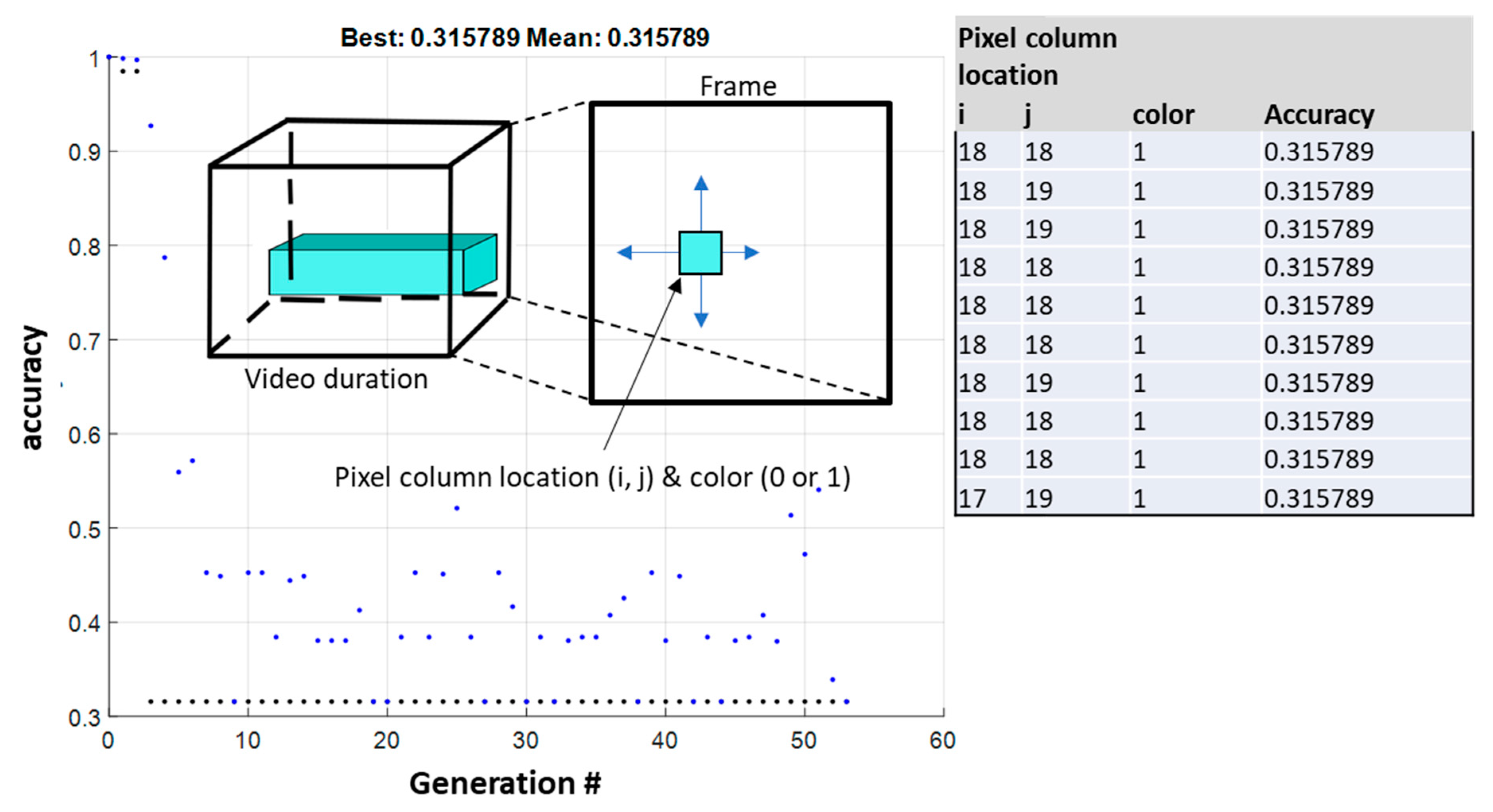
The second step included a similar procedure for locating, which are the coordinates of the “pixel column” on the frame plane and its color (zero or one), in order the achieve the maximum accuracy drop. The implementation included minor changes to the GAs parameters, such as its population size, which was reduced to 10 coordinate–color pairs. After 50 generations, the algorithm stopped, as no significant changes in the value of the objective function were observed. The results indicated a “pixel column” with coordinates (18,18) and a value of one, causing a significant drop in the model’s accuracy, which was 32% compared to the model prediction on the unmodified inputs (Figure 8), again using an order of magnitude of fewer iterations compared to a simple grid search.

With the above-mentioned steps completed, the logical continuation for constraining the perturbation into a single pixel was to combine the previous approach and change the pixel (18,18) at the frame position 25 to the value one. This did not, however, result in any changes in the accuracy. Thus, a third step was added in order to find the smallest pixel column possible, which can cause the same accuracy to drop as achieved in the previous step. The optimization problem in this case was to identify the length and location of this pixel column, which will cause the biggest accuracy drop. The position and length of the column were constrained between 1 and 200 pixels as during a preliminary hand-crafted search, these were indicated as the most promising candidates. Once again, a GA was implemented with a population of 10 individuals of position–length individuals. The results indicate that a column with a length of 194 pixels with a value of one staring at frame position 11 can have the same accuracy drop as step 2. In the following figure, the progress of the GA is depicted along with the final population (Figure 9). Note that the score does not correspond to the accuracy as another term was added to the objective function, ensuring that the length will be kept as small as possible.

Moving on, the corresponding HEAVI attacks for the case of SAW were straightforward to implement. In this case, as the hardware acceleration was available for the given CNN, a simple grid search was implemented for finding how much each pixel location and value (one or zero) could compromise the accuracy of the model. The accuracy results are depicted in the following figure (Figure 10) for a class-balanced set of 800 images sampled from a bigger one of 150,000 frames, which is not balanced (EP-13%, GW-58%, NW-6%, and PP-23%). For both color values, the accuracy was increasing radially, away from ground zero (pixel location for which the lowest accuracy value was observed). The calculation of the accuracy is made herein considering the predictions of the model on the unmodified samples as the ground truth. With the following pixel coordinates identified, the best candidates were used on the actual test set of 150,000 images. The accuracy result on this set for the pixel coordinates 19 and 20 and pixel value equal to 0, was 97%, while for the pixel coordinates 20 and 18 and pixel value equal to 1, the accuracy result was 44%.

3.2. Blind-Attacks—AWGN

AWGN attacks were performed frame-wise for both the RSW and SAW case, using the corresponding build-in function of MATLAB. The “intensity” of the noise is controlled by adjusting the SNR value, which ranges between 10 and 60 dB. For the case of RSW, the noise is applied on the flattened video vectors as depicted in the following figure (Figure 11). The result was a sharp decrease in accuracy, which as with the previous HEAVI attacks on the RSW, bottomed out at 32% for an SNR value of 27 dB.

For the SAW case as with the HEAVI attack, the noise was added to a sample of 800 images for calculating the effect on the accuracy. The noise levels varied as previously between 10 and 60 dBs and the accuracy had a sudden drop between 30 and 35 dB and finally reached its smallest value of 27% percent after a small flat spot, which is very close to the actual distribution of a single class (25%). The figure below (Figure 12) depicts the previously mentioned results. With the accuracy being calculated on the 800-image sample, it was also calculated on the test set of images for 40, 30, 20, and 10 dB, to validate that it follows more or less the same trend. Thus, the resulting accuracy scores were 98, 85, 62, and 17%, respectively, qualitatively validating the same behaviors.

3.3. Domain-Informed Attacks

For the domain-informed attacks, as already mentioned, an identical approach followed for both the RSW and SAW cases. The 2 × 2 kernel was multiplied element-wise with a gain factor ranging from 0.01 to 1 and the accuracy was calculated for the two cases using the datasets that have been used in the previous attacks. The operation of convolution keeps only the central part, which means that the resulting matrix has the same size as the original image. Furthermore, white Gaussian noise (SNR: 50 dB) was added to each convoluted frame as calculated on the original to compensate for the blur effect that this kind of box-like filter causes. The following figure (Figure 13) depicts the accuracy changes vs. the kernel gain for the RSW case.

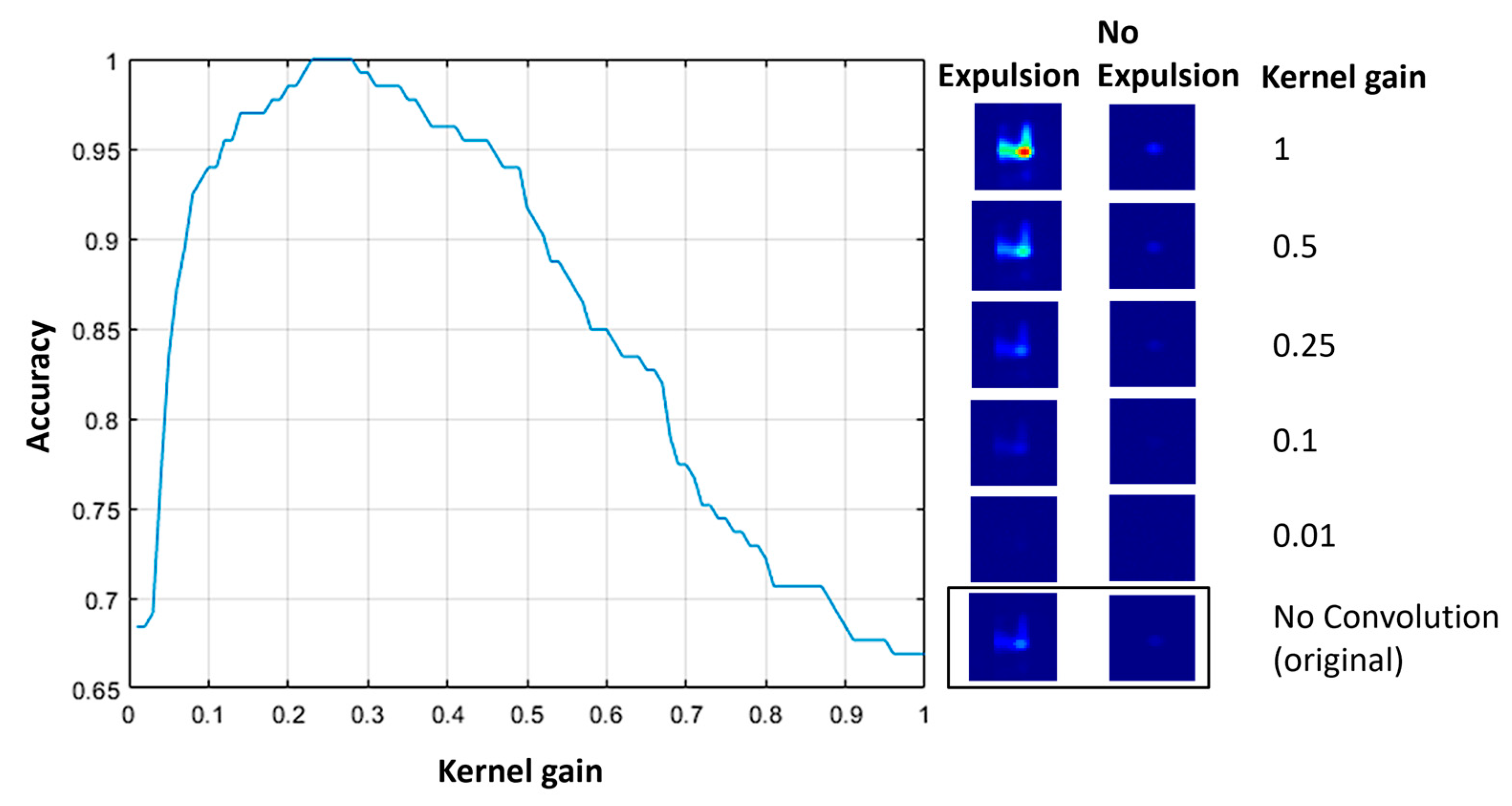
For the SAW case, the accuracy was calculated the same as previously on a small sample (800 images), as depicted in the following figure (Figure 14). The accuracy on the test set, as defined in previous paragraphs (150,000 frames), was calculated for the gain values of 0.01, 0.1, 0.25, 0.3, and 0.4, and resulted in 58%, 9%, 96%, 54%, and 16%. In addition, the accuracy is changing linearly and it is quantized for different values of the gain.

4. Discussion

4.1. Result Analysis

Regarding the attacks described in the previous section, the HEAVI attack on the RSW model was capable of compromising its performance completely. This is due to the fact that a 32% accuracy means that the attack entirely shifted the predictions of the majority class, which was the “No Expulsion” class. Beyond the raw metrics concerning the performance of the attack, its structure is important to be analyzed as it reveals insights into the feature extraction mechanisms and the decision-making of the corresponding model. Thus, in this case, the value, position, and length of the injected pixel column indicate that the dimensions that the PCA algorithm identifies as the ones having the highest variance are located temporary-wise at the start of the video and spatial-wise, approximately, at the middle of the frame. This is typically where the process thermal signature appears in each frame and when its maximum temperature is achieved during welding, as already analyzed in [3]. Regarding decision-making, as hypothesized in the corresponding “Domain-Informed Attacks”, it is indeed dependent on the pixel value for the previously mentioned dimensions (pixel coordinates where the thermal signature appears), meaning that the higher the pixel value, the more probable it is in the corresponding video to be placed in the “Expulsion” class.

Looking at SAWs HEAVI attack results, the first thing that is obvious is that both for the zero and one pixel-value injections, the area for which these are having the most significant effect on the model’s accuracy is pretty much the same, with the area corresponding to the zero pixel-value injections, to be slightly smaller and having a milder effect (Figure 10). Furthermore, the area that is affected by the injections seems to be located within the spatial margins of the process thermal signature and more specifically, toward the welding electrode or otherwise the upper right corner of the image. This could mean that the CNNs filters are configured for extracting features concerning this area in particular, which is good on one hand, as the model indeed considers the area of the image where the seam’s cooldown is more profound, but bad at the same time, as the model can be easily modified by utilizing a small perturbation. Same as with the RSW case, the pixel intensity, which depends on the temperature, seems to be strongly correlated with defects, as already implicitly hypothesized in [32]. Finally, another artifact is that the severity of the accuracy drop for both pixel values fades away with moving further away from the point with the greatest impact.

Moving on with the AWGN attacks, it cannot be left undiscussed the fact that both models are quite robust to SNR levels as low as 40 dBs. While for the case of SAW, making assumptions on how this is achieved is not trivial, and for the RSW case, this can be justified to some extent by looking at the flattened video vectors and the temporal profile of the pixels that are located within the area where the thermal signature of the process typically appears (Figure 14). So, as already hypothesized in the case of the HEAVI attacks, the classification is based on the values of certain pixels that are compared to a threshold. That is, the actual noise is added on the video ‘vector’ and not specifically on these video vector dimensions where the thermal signature of the process is registered. Thus, it requires quite low SNR values to increase the chances of inflicting “damage”, as most of the dimensions are corresponding to background pixels, which represent random noises by default. Thus, the addition of noise everywhere just amplifies the background noise for high SNR values. Another finding in the context of this AWGN attack for the RSW case, is that the spatio-temporal dimensions that the feature extraction algorithm weights the most, and the pixel threshold values upon which the model base its decisions, could be defined with relative ease using simple handcrafted rules. Thus, it could be stated with caution that adding noise specifically to an area of an imaginary box located at the middle of the frame and stretching it in the temporal dimension for a duration similar to the length of the HEAVI’s attack “pixel-column” could inflict the same “damage” to the RSW model. With that in mind, an exploratory attempt of adding a 5 × 5 × 197 pixel “noise” rectangular box of 20 dB around the pixel (18,18) resulted in an accuracy of 90%, while for a 15 dBs SNR, the accuracy eventually dropped to 32%. Increasing this box’s cross-section also resulted in an accuracy drop, but the same did not happen when increasing its length. Finally, in the same vein, creating a “noise-pixel-column” with the same specification as the one in the corresponding HEAVI attack did not have any effect, even for quite low SNR values.

Coming back to the SAW case, the AGWN attack had a similar effect. Increasing the amount of noise resulted in general in a decrease in the accuracy; however, this occurred in a non-linear fashion. Similarly to the RSW case, the capture frames are including pixels in the background that are following a white noise pattern. Thus, again a lot of noise is required to be added in order to inflict significant damage to the model’s accuracy as specific areas/pixels, as already identified in the HEAVI attack, are weighted more than others for the decision-making. To justify this hypothesis to a certain extent, as with the RSW case above, a similar experimentation of adding a 5 × 5 noise pad around the pixel (20,18), as identified in the HEAVI attack, was implemented. The resulting accuracy for an SNR level of 20 dBs was slightly higher (73%) compared to the corresponding one on the full-frame AWGN attack on the test set, which further justifies the claims made in the context of the HEAVI attack.

With the results of the “Blind-Attacks” analyzed, it cannot be ignored the fact that for both the RSW and SAW cases, either by adding noise or simply by forcing a pixel or a number of pixels to have the maximum value possible for specific spatiotemporal dimensions is what “fools” the model of thinking that high temperatures above certain thresholds are depicted in the image. This is the essence of the “Domain-Informed Attacks”, which in simple words are amplifying the image features and simultaneously adding a blur, which aids in smoothening the transitions between image features with low and high values. Analyzing the “Domain-Informed Attacks” for the RSW case, in Figure 13 the accuracy starts from 68% and reaches 100% for a gain value of 0.25. Both numbers are not random, with 68% accuracy to represent a complete shift of the minority class (expulsion) as the kernel heavily reduces the intensity of the thermal signatures, and 100% accuracy to validate that the blurring made by the box kernel does not cause any changes. For high gain values even greater compared to the ones investigated, the accuracy did not drop as much as to indicate a complete shift of the majority class (no-expulsion).

For the SAW case, having in mind that the data sample was balanced class-wise, it was easy to identify which gain value caused one or more classes to be misclassified. A total misclassification was achieved for a low gain value (0.1), so low in fact that it decreased the image intensity significantly compared to the original (Figure 14). Based on the previous hypothesis, that the pixel intensity mainly determines the classification output, each of images belonging to the GW, PP, and EP classes were kind of demoted into the class with the next lower intensity “threshold” for a kernel gain of 0.1. However, if that is the case, it cannot be explained for how the NW was classified.

Table 4. Macroscopic overview of attacks impact.

Attack Type	Process	Space Span	Time Span	Perturbation Value	Impact
HEAVI	RSW	One pixel	Throughout welding (~200 ms)	Max pixel value	Model predicts randomly
HEAVI	SAW	One pixel	-	Max pixel value	The model can guess right two out of four trials
AWGN	RSW	Entire frame	Throughout monitoring duration	Random noise of 27 dB	Model predicts randomly
AWGN	SAW	Entire frame	-	Random noise of 29 dB	Model’s prediction same as a random guess
Domain-informed attacks	RSW	Entire frame	-	2 × 2 kernel of 0.01 (soften image features	Model predicts randomly
Domain-informed attacks	SAW	Entire frame	-	2 × 2 kernel of 1 (amplify image features)	Model predicts randomly

summarizes all the macroscopic results.

4.2. Performing the Attacks and Identify and Correcting Adversarial Inputs

In a real-world scenario, crafting black-box attacks can be performed in two ways [36]. The first one requires as a first step to “eavesdrop” for collecting several input–output pairs for training a substitute model and testing it. Then, this substitute model is utilized in the context of a white-box attack in order to craft the adversarial inputs. The second one is based simply on a query feedback mechanism, where the attacker continuously creates adversary inputs and queries the model. Consequently, looking at the proposed framework in Section 2, the attacks could be applied using the last strategy following a number of modifications. These strategies are related to optimization procedures that are used for developing the adversary input. As such, for the ones utilizing a simple grid-search, a more efficient algorithm could be used for minimizing the overall number of queries, such as GA or handcrafted ones. However, even if a very low number of queries is eventually needed, another problem arises from the very nature of applications for defect detection and quality assessment in general. As such, in case that the model is deployed in an industrial production environment, where the frequency of a defect or an out-of-spec part is not the norm, the creation of data batches using equally distributed to all the quality classes would be difficult. This in turn can lead to prolonged queries, increasing the chances for the malicious software to be detected. Finally, the most convenient scenario for implementing these attacks is what has already been mentioned in Section 2, which is where the attacker has access to the actual service that hosts the model. This not only does not require the attacker to minimize its queries but also limits the active interaction of the attacker with the system, as it only requires eavesdropping and thus minimizes the chances of being discovered before the optimal adversarial input has been crafted.

Identifying and correcting an adversarial input created using the previously mentioned attacks is quite obvious for some of the cases, while other additional information is needed apart from the input data. HEAVI attacks could be detected for example by performing simple image thresholding, given the fact that the upper and lower limits are known for a given application and that pixel saturation has a very low probability of happening. Another out-of-the-box method could be searching for the maximum or minimum value of pixels. Of course, data visualization could be utilized by an expert for identifying adversary inputs and marking them for rejection, but this would be impractical and it is not always feasible, given the fact that the HEAVI attacks on the RSW process just inject a single-pixel perturbation for about 200 ms. On the other hand, AWGN attacks cannot be identified as easily because knowledge about the added noise is typically needed and even then, removing the added noise is not trivial by any means. Of course, again low SNR values could be identified visually but not removed. Last but not least the “Domain-Informed Attacks” are the hardest to detect both visually and “algorithmically”. This is because they are appearing as visually similar to an image corresponding to the defective class, at least for the gain values that are not resulting in unnatural IR process signatures. In addition, the fact that the entire perturbation is applied to the entire image does not leave any part of it unchanged that could be used as a reference point for any identification and correction attempts. The only case where their identification could be possible is when the potential adversarial inputs are compared to the input process parameters. However, this will require the creation of auxiliary models for assessing if an input corresponds to the given input parameters. Finally, as regards all the previously mentioned attacks, metrics such as the L2 norm for measuring the similarity of the input vector with a given class distribution could be utilized for identifying an adversarial input as long as the norm of the adversarial input does not result in a norm that falls within a class distribution. This was not, however, the case for the adversarial inputs that appeared to be visually similar to the original ones (e.g., AWGN and domain-informed attacks) and even for the HEAVI attacks, at least for the RSW case.

5. Conclusions

In this study, two machine learning models purposed for two quality monitoring tasks in the context of two welding applications (RSW and SAW) and under the same software and hardware framework were used for crafting three different adversarial attack methods. Most of the attacks were able to compromise the accuracy of the corresponding models down to the point where the prediction ability of the models was no better than a random guess, even for the case of a deep learning model, which has been trained upon hundreds of thousands of examples.

More specifically, the temperature value and its temporal profile during welding, or otherwise the pixel intensity for these quality-monitoring cases, has been identified as a major factor upon which the decision-making is performed from both models.

In the context of the adversarial attacks for RSW, this means that the model’s accuracy is affected if the intensity of the pixels, at the image area where the thermal signature of the process appears, is changed for as long as the welding system provides energy to the spot and not during the cooldown. To this end, localized attacks, such as single-pixel/maximum pixel-value attacks, are causing significant drops in the targeted model’s accuracy and can be easily detected with threshold-based rules. On the other hand, mild perturbations in the form of localized noise or the selective amplification of image features are able to inflict moderate damage, which not only could be hardly detectable, but also, could be hardly correctable.

Similar conclusions can be drawn for the SAW case. Herein, amplifying and not just changing the pixels’ intensity around a specific area in a frame could cause the model to misclassify the input.

Regarding the attacks from an implementation perspective, single-pixel attacks and in general localized ones are the most difficult to tune and would require as much data as possible. On the contrary, domain knowledge attacks that are targeting on amplifying in general the intensity of specific image features can be applied with nearly no tunning at all, and they would most probably achieve a measurable drop in the performance of the targeted model.

The results of this study do not define a general rule that could limit the accuracy of a quality monitoring system based on infrared images for welding, but they can help toward creating a framework through which adversarial attacks’ tuning can be avoided.

However, the span of the manufacturing processes themselves is currently limited to SAW (seams) and RSW (spots). Additionally, despite the fact that this is a study on how the attacks affecting each model have been conducted, the means for detecting and defending them were only mentioned. Thus, future work is expected, aiming at developing a framework that is able to quantitatively distinguish potential adversarial inputs without utilizing user-defined thresholds and providing solutions during the training of a model for making it invulnerable to the majority of perturbations. The actual injection of the attacks having access to the model will have to be discussed as well.

References

1. The American Welding Society Inc. AWS WI: 2015 Welding Inspector Handbook; American Welding Society: Miami, FL, USA, 2015. [Google Scholar]
2. Montgomery, D.C. Introduction to Statistical Quality Control; John Wiley & Sons: Hoboken, NJ, USA, 2007. [Google Scholar]
3. Stavropoulos, P.; Sabatakakis, K.; Papacharalampopoulos, A.; Mourtzis, D. Infrared (IR) quality assessment of robotized resistance spot welding based on machine learning. Int. J. Adv. Manuf. Technol. 2022, 119, 1785–1806. [Google Scholar] [CrossRef]
4. Stavropoulos, P.; Bikas, H.; Sabatakakis, K.; Theoharatos, C.; Grossi, S. Quality assurance of battery laser welding: A data-driven approach. Procedia CIRP 2022, 111, 784–789. [Google Scholar] [CrossRef]
5. Kloukiniotis, A.; Papandreou, A.; Lalos, A.; Kapsalas, P.; Nguyen, D.V.; Moustakas, K. Countering adversarial attacks on autonomous vehicles using denoising techniques: A Review. IEEE Open J. Intell. Transp. Syst. 2022, 3, 61–80. [Google Scholar] [CrossRef]
6. Anastasiou, T.; Karagiorgou, S.; Petrou, P.; Papamartzivanos, D.; Giannetsos, T.; Tsirigotaki, G.; Keizer, J. Towards Robustifying Image Classifiers against the Perils of Adversarial Attacks on Artificial Intelligence Systems. Sensors 2022, 22, 6905. [Google Scholar] [CrossRef] [PubMed]
7. Statista Site. Available online: https://www.statista.com/chart/26148/number-of-publicized-ransomware-attacks-worldwide-by-sector/ (accessed on 10 December 2022).
8. Huelsman, T.; Peasley, S.; Powers, E.; Robinson, R. Cyber risk in advanced manufacturing. Deloitte MAPI 2016, 53. [Google Scholar]
9. Abuhasel, K.A.; Khan, M.A. A secure industrial Internet of Things (IIoT) framework for resource management in smart manufacturing. IEEE Access 2020, 8, 117354–117364. [Google Scholar] [CrossRef]
10. Shahbazi, Z.; Byun, Y.C. Integration of Blockchain, IoT and machine learning for multistage quality control and enhancing security in smart manufacturing. Sensors 2021, 21, 1467. [Google Scholar] [CrossRef] [PubMed]
11. Zhang, B.; Magaña, J.C.; Davoodi, A. Analysis of security of split manufacturing using machine learning. In Proceedings of the 55th Annual Design Automation Conference, San Francisco, CA, USA, 24–29 June 2018; pp. 1–6. [Google Scholar]
12. Zellinger, W.; Wieser, V.; Kumar, M.; Brunner, D.; Shepeleva, N.; Gálvez, R.; Langer, J.; Fischer, L.; Moser, B. Beyond federated learning: On confidentiality-critical machine learning applications in industry. Procedia Comput. Sci. 2021, 180, 734–743. [Google Scholar] [CrossRef]
13. Barreno, M.; Nelson, B.; Joseph, A.D.; Tygar, J.D. The security of machine learning. Mach. Learn. 2010, 81, 121–148. [Google Scholar] [CrossRef] [Green Version]
14. Qayyum, A.; Qadir, J.; Bilal, M.; Al-Fuqaha, A. Secure and robust machine learning for healthcare: A survey. IEEE Rev. Biomed. Eng. 2020, 14, 156–180. [Google Scholar] [CrossRef]
15. Farahmandi, F.; Huang, Y.; Mishra, P. System-on-Chip Security; Springer: Berlin/Heidelberg, Germany, 2020; pp. 173–188. [Google Scholar]
16. Kumar, S.; Sahoo, S.; Mahapatra, A.; Swain, A.K.; Mahapatra, K.K. Security enhancements to system on chip devices for IoT perception layer. IEEE Int. Symp. Nanoelectron. Inf. Syst. 2017, 151–156. [Google Scholar]
17. Papernot, N.; McDaniel, P.; Sinha, A.; Wellman, M. Towards the science of security and privacy in machine learning. arXiv 2016, arXiv:1611.03814. [Google Scholar]
18. Su, J.; Vargas, D.V.; Sakurai, K. One pixel attack for fooling deep neural networks. IEEE Trans. Evol. Comput. 2019, 23, 828–841. [Google Scholar] [CrossRef] [Green Version]
19. Gao, L.; Zhang, Q.; Song, J.; Liu, X.; Shen, H.T. Patch-wise attack for fooling deep neural network. In European Conference on Computer Vision; Springer: Cham, Switzerland, 2020; pp. 307–322. [Google Scholar]
20. Papernot, N.; McDaniel, P.; Goodfellow, I.; Jha, S.; Celik, Z.B.; Swami, A. Practical black-box attacks against machine learning. In Proceedings of the ACM on Asia Conference on Computer and Communications Security, Abu Dhabi, United Arab Emirates, 2–6 April 2017; pp. 506–519. [Google Scholar]
21. Din, S.U.; Akhtar, N.; Younis, S.; Shafait, F.; Mansoor, A.; Shafique, M. Steganographic universal adversarial perturbations. Pattern Recognit. Lett. 2020, 135, 146–152. [Google Scholar] [CrossRef]
22. Wei, Z.; Chen, J.; Wei, X.; Jiang, L.; Chua, T.S.; Zhou, F.; Jiang, Y.G. Heuristic black-box adversarial attacks on video recognition models. Proc. AAAI Conf. Artif. Intell. 2020, 34, 12338–12345. [Google Scholar] [CrossRef]
23. Jiang, L.; Ma, X.; Chen, S.; Bailey, J.; Jiang, Y.G. Black-box adversarial attacks on video recognition models. In Proceedings of the 27th ACM International Conference on Multimedia, Nice, France, 21–25 October 2019; pp. 864–872. [Google Scholar]
24. Wei, X.; Liang, S.; Chen, N.; Cao, X. Transferable adversarial attacks for image and video object detection. arXiv 2018, arXiv:1811.12641. [Google Scholar]
25. Li, S.; Aich, A.; Zhu, S.; Asif, S.; Song, C.; Roy-Chowdhury, A.; Krishnamurthy, S. Adversarial attacks on black box video classifiers: Leveraging the power of geometric transformations. Adv. Neural Inf. Process. Syst. 2021, 34, 2085–2096. [Google Scholar]
26. James, J.Q.; Hou, Y.; Li, V.O. Online false data injection attack detection with wavelet transform and deep neural networks. IEEE Trans. Ind. Inform. 2018, 14, 3271–3280. [Google Scholar]
27. Meenakshi, K.; Maragatham, G. A self supervised defending mechanism against adversarial iris attacks based on wavelet transform. Int. J. Adv. Comput. Sci. Appl. 2021, 12. [Google Scholar] [CrossRef]
28. Sarvar, A.; Amirmazlaghani, M. Defense against adversarial examples based on wavelet domain analysis. Appl. Intell. 2022, 1–17. [Google Scholar] [CrossRef]
29. Tamizhiniyan, S.R.; Ojha, A.; Meenakshi, K.; Maragatham, G. DeepIris: An ensemble approach to defending Iris recognition classifiers against Adversarial Attacks. In International Conference on Computer Communication and Informatics; IEEE: Coimbatore, India, 2021; pp. 1–8. [Google Scholar]
30. NIT Site. Available online: https://www.niteurope.com/tachyon-1024-ucamera/ (accessed on 10 December 2022).
31. MATLAB Deep Learning Toolbox Site. Available online: https://www.mathworks.com/help/pdf_doc/deeplearning/nnet_ref.pdf (accessed on 1 December 2022).
32. Stavropoulos, P.; Papacharalampopoulos, A.; Sabatakakis, K. Online Quality Inspection Approach for Submerged Arc Welding (SAW) by Utilizing IR-RGB Multimodal Monitoring and Deep Learning. In International Conference on Flexible Automation and Intelligent Manufacturing; Springer: Cham, Switzerland, 2023; pp. 160–169. [Google Scholar]
33. Tuptuk, N.; Hailes, S. Security of smart manufacturing systems. J. Manuf. Syst. 2018, 47, 93–106. [Google Scholar] [CrossRef]
34. Guo, C.; Gardner, J.; You, Y.; Wilson, A.G.; Weinberger, K. Simple black-box adversarial attacks. In International Conference on Machine Learning; PMLR: Long Beach, CA, USA, 2019; pp. 2484–2493. [Google Scholar]
35. Deep, K.; Singh, K.P.; Kansal, M.L.; Mohan, C. A real coded genetic algorithm for solving integer and mixed integer optimization problems. Appl. Math. Comput. 2009, 212, 505–518. [Google Scholar] [CrossRef]
36. Akhtar, N.; Mian, A.; Kardan, N.; Shah, M. Advances in adversarial attacks and defenses in computer vision: A survey. IEEE Access 2021, 9, 155161–155196. [Google Scholar] [CrossRef]
Figure 1. Quality monitoring platform architecture.
Machines 11 00298 g001
Figure 2. Monitoring setup for the RSW process.
Machines 11 00298 g002
Figure 3. Monitoring setup for the SAW process.
Machines 11 00298 g003
Figure 4. SAW residual CNN model high-level architecture diagram.
Machines 11 00298 g004
Figure 5. Adversarial attack framework. * The optimization module is not required in all attacks.
Machines 11 00298 g005
Figure 6. Types of attacks in monitoring: Single frame attack (a), Single pixel attack (b), localized attack (c), Random noise attack (d), Concealed physics–based noise (e).
Machines 11 00298 g006
Figure 7. Genetic algorithms converge progress—searching for the frame position and color that compromise the most of the RSW model’s accuracy (integrated table shows the best generation).
Machines 11 00298 g007
Figure 8. Genetic algorithms converge progress—searching for the pixel column location and pixel color on a 32 × 32 pixel grayscale frame that compromises the most the RSW model’s accuracy (integrated table shows the best generation).
Machines 11 00298 g008
Figure 9. Genetic algorithms converge progress—pixel column position and length search.
Machines 11 00298 g009
Figure 10. Classification accuracy depends on the location of a single pixel’s perturbation for the case of SAW—results are on the 800-image sample.
Machines 11 00298 g010
Figure 11. Classification accuracy of the NN model depending on the added noise levels for the case of RSW along with a random frame for which noise has been added for different SNR values.
Machines 11 00298 g011
Figure 12. Classification accuracy of the CNN model depending on the added noise levels for the case of SAW along with a random frame from the GW class for which noise has been added for different SNR values.
Machines 11 00298 g012
Figure 13. Classification accuracy of the NN model depending on the 2 × 2 kernel gain factor for the RSW case along with two random frames from the two classes (expulsion and no expulsion) that have been convolved with kernels having different gain values.
Machines 11 00298 g013
Figure 14. Classification accuracy of the CNN depending on the 2 × 2 kernel gain for the SAW case along with a random frame from the GW class that has been convolved with kernels having different gain values.
Machines 11 00298 g014