Abstract
In order to improve the accuracy of tool wear prediction, an attention-based composite neural network, referred to as the ConvLSTM-Att model (1DCNN-LSTM-Attention), is proposed. Firstly, local multidimensional feature vectors are extracted with the help of a one-dimensional convolutional neural network (1D-CNN), which avoids the loss of wear features caused by manual feature extraction. Then the temporal relationship learning between multidimensional feature vectors is performed by introducing a long short-term memory (LSTM) network to make up for the lack of long-short distance dependence of the captured sequence of the CNN network. Finally, an attention mechanism is applied to strengthen the ability to extract key information from tool-wearing temporal features. The proposed ConvLSTM-Att model is trained with the measured tool wear data and then performs as a tool wear predictor. The model is compared with several state-of-the-art models on the PHM tool wear data sets. It significantly outperforms the other models in terms of prediction accuracy, but with similar computational complexity.
1. Introduction
As a result of China’s vigorous promotion of the Manufacturing Industry 2025, the machinery manufacturing industry has increasingly higher requirements for intelligence [1,2]. As an important part of machinery production and processing, the degree of wear and tear on tools severely affects the accuracy of workpieces and the manufacturing costs of enterprises. Most of the traditional tool changing methods are based on experience, determining the timing of tool stopping and tool changing. Changing a tool too early will cause wastage of the tool [3], whereas changing a tool too late will reduce the quality of a workpiece and lead to scrapping. During the machining process, timely and accurate prediction of tool wear is beneficial to both improving the machining accuracy of products and reducing the manufacturing and labor costs of enterprises. Therefore, intelligent and accurate prediction of tool wear has become an important topic.
Direct and indirect measurements are the two main approaches to tool wear prediction [4]. The direct measurement approach requires off-line measurement of the tool between machining intervals, which greatly affects the coherence of machining and is difficult to apply in production practice. The indirect measurement method is primarily used to predict tool wear by mining and analyzing the relationship between the data taken during machining and the tool wear data. However, the data acquired during machining is subject to noise in the industrial environment, which reduces the validity of the data [5].
Traditional machine learning approaches, such as artificial neural networks [6], fuzzy logic [7], the hidden Markov model and support vector machine, as well as metaheuristic approaches [8,9], can be implemented for tool wear prediction, but the prediction accuracy is generally low [10]. It is difficult for traditional machine learning approaches to predict the true data directly from the measured data [11]. Therefore, some preprocessing methods such as time-frequency domain analysis [12], principal component analysis (PCA) [13], and empirical modal decomposition (EMD) [14] are usually required for the data. However, extracted features are easy to underweight in the data that reflect tool wear, and the tool wear data are essentially time series, so the above approaches cannot tap the time-series features between different data samples.
In recent years, deep learning [6], with its excellent ability to automatically learn features, has provided a new idea for dealing with large-scale mechanical data [15]. It is widely used in the fields of computer vision [16], speech recognition [17], natural language processing [18], and mechanical fault diagnosis [19]. The tool wear prediction model based on deep learning has significantly improved the accuracy of tool wear prediction by virtue of its powerful data processing as well as feature extraction capability [19].
Convolutional neural networks (CNN) have excellent performance in processing data, text, and image recognition. They can analyze the original data and extract high-dimensional hidden features, effectively circumventing the problems that arise from handcrafted feature extraction. Kothuru et al. [20] established a CNN-based tool condition prediction model for tool wear prediction by analyzing the spectral characteristics of the acoustic signals during machining. Xu et al. [21] used CNN to extract features from the collected vibration data during machining and designed an extended convolutional residual block and fully connected layer to achieve effective prediction of tool wear. The long short-term memory (LSTM) network is a type of recurrent neural network that effectively avoids the vanishing gradient problem in the recurrent neural network and better mines the temporal features between different temporal data sets [22]. In order to capture the long-term dependence of tool wear data, Zhao et al. [23] presented a deep LSTM model to predict tool wear by regression, confirming that LSTM has certain advantages compared with conventional recurrent neural networks in processing temporal data. Cai et al. [24] proposed a hybrid model based on LSTM to extract the temporal features from the raw sequence data through a designed stacked LSTM and finally in a nonlinear regression model to obtain the predicted tool wear. Chan et al. [25] combined CNN and LSTM and proposed an LSTM-CNN model. It uses CNN to extract tool wear features, and then mines the temporal features of tool wear by LSTM, to achieve effective prediction of tool wear. Schwendemann et al. [26] propose a deep learning method based on transfer learning. This method uses the windowed envelope, de-noising, and normalization processing of low-frequency sensor data to form the intermediate domain image and uses CNN and LSTM to perform the estimation of remaining useful life and realize effective transfer learning between different bearing types. Qiao et al. [27] collected vibration and current signals as well as tool wear as input to construct a training data set and input the features extracted by the multi-scale convolutional LSTM model to a bidirectional LSTM model to predict tool wear. It meets the requirements of high accuracy and low latency. Attention is a weight assignment mechanism that improves learning accuracy by learning to continuously update the attention weights corresponding to different features and to ignore unimportant signals [28]. Huang et al. [29] combined CNN with attention and proposed a multiscale CNN based on attention fusion, which will improve the accuracy of tool wear prediction by extracting tool wear data through multi-layer convolution as input and passing them to a multilayer attention mechanism.
The above methods consider, to some extent, the feature extraction of tool wear data in spatial and temporal dimensions and the contribution of different data to tool wear in the spatial dimension, respectively. However, they do not consider the different specifics of different data features fused with spatial and temporal dimensions for tool wear prediction. In order to enhance the extraction of key information while fusing different dimensional features of the measured data, we propose a composite neural network model based on an attention mechanism. The model uses a 1D-CNN neural network to extract multidimensional feature data. Then, in order to fuse the features in the temporal dimension, an LSTM network is introduced to extract sequential features by learning the temporal relationship between multidimensional features through an LSTM layer. Finally, the ability of the model to obtain key wear data features is improved with the help of the attention mechanism, resulting in an efficient and accurate prediction of tool wear.
2. Composition of the Prediction Model
2.1. One-Dimensional Convolutional Neural Network (1D-CNN)
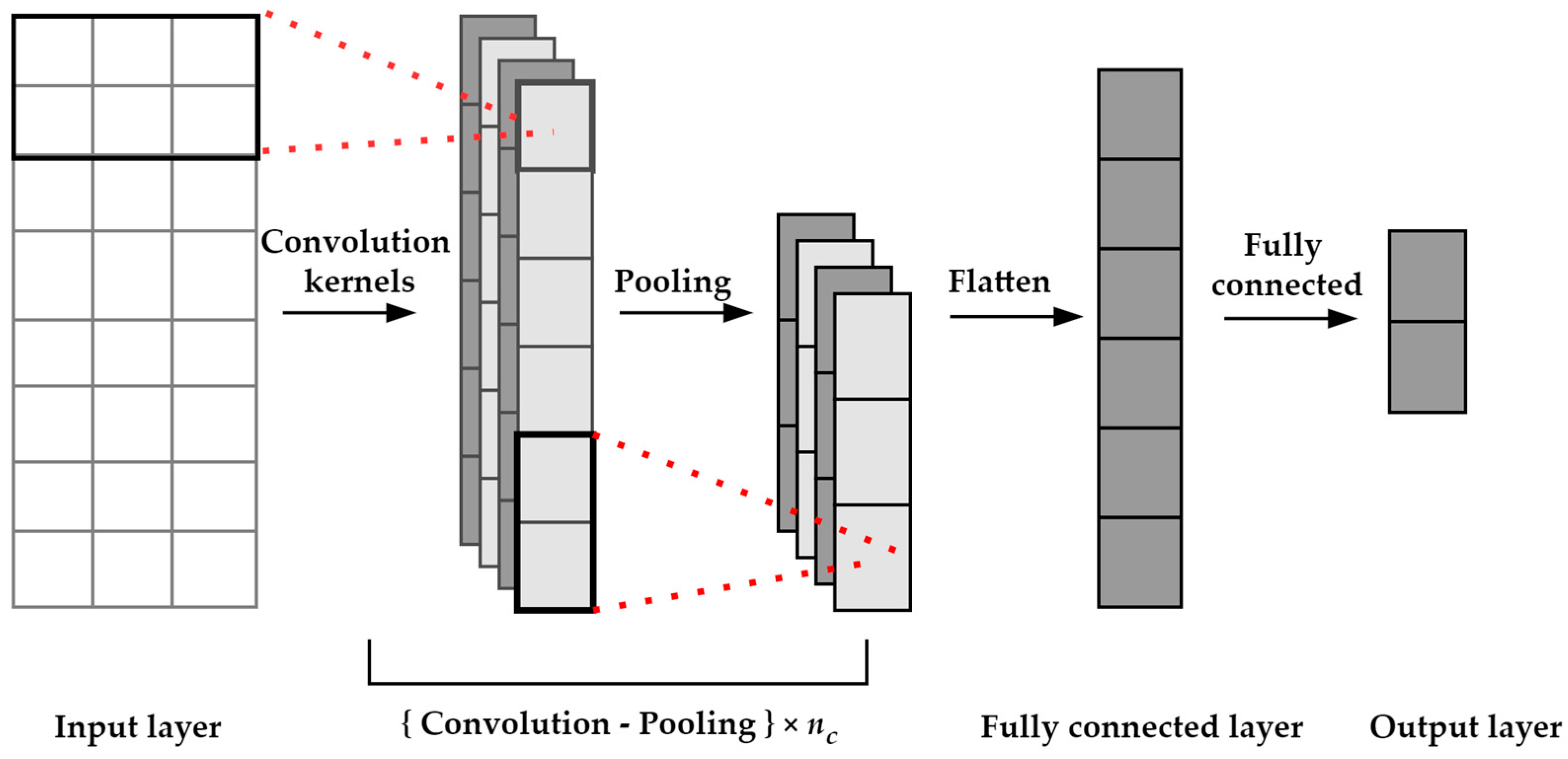
The CNNs are feedforward neural networks with special structures that excel at image and speech recognition. Among them, the one-dimensional convolutional neural network (1D-CNN) has excellent performance in processing text data [30]. The 1D-CNN structure is shown in Figure 1, which is composed of three major layers, namely, the convolutional layer, the pooling layer, and the fully connected layer [31]. The convolutional layer slides with the elements in the perceptual field at a prespecified step and makes a nonlinear mapping through the activation function to extract the feature vectors. It is the core layer of the whole network. The pooling layer reduces the dimensions of the feature vectors outputted from the convolutional layer and keeps the most significant ones locally to reduce operations. The fully connected layer is a fully connected neural network, which does a nonlinear transformation of the feature vectors to generate the specified dimensions and passes them on to generate the classification result [32].
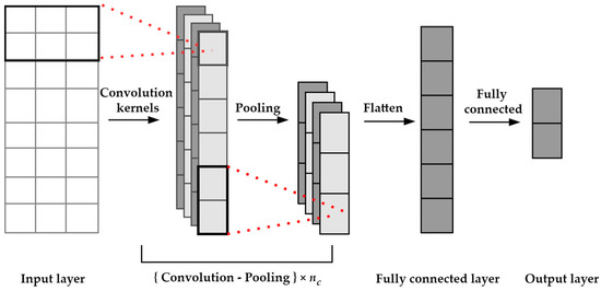
Figure 1.
Network structure of the 1D-CNN. is the number of the convolution-pooling layers.
2.2. Long Short-Term Memory (LSTM) Network
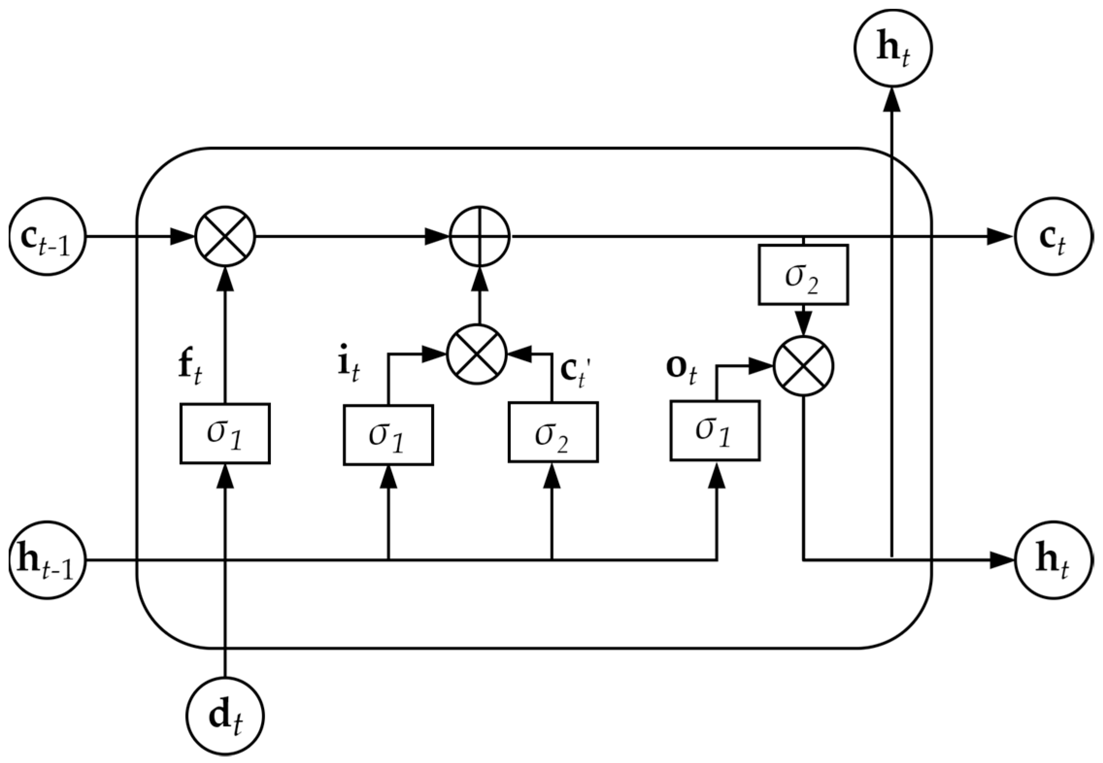
The LSTM is a recurrent neural network with long-term and short-term memories between feature vectors, and the memories can be dynamically adjusted with the input, which greatly solves problems such as memory degradation caused by too long sequences [33]. At the same time, LSTM can also solve the problem of vanishing gradients that exists in conventional recurrent neural networks and can better exploit the temporal relationship between tool and feature vectors. The core idea of LSTM is to introduce input gates, forgetting gates, and output gates for each memory unit [34]. The structure of LSTM is shown in Figure 2.

Figure 2.
LSTM network structure.
The forget gate decides what is deleted from the memory cell according to the previous hidden layer state , is the LSTM number of hidden layer neurons, with the current input , being the number of convolution kernels, by the sigmoid function. The input gate decides what to save from the previous hidden statewith the current input according to the sigmoid function and gets a candidate parameter according to the tanh function. Combining the forget gate with the input gate, the current state of the memory cell is updated. The output gate uses the sigmoid function to determine what is output from and . The outputs of the output gate are combined with which is processed by the tanh function to selectively output the hidden layer state at the current time. The LSTM model is given by
where is the forget gate output at the time , is the input gate output at time , is the state of the memory cell at the time , is the output gate output at the time , is the sigmoid function, is usually selected as the tanh function, is the hidden layer state at time , is the input at time , , , and are the weight matrices of , , , and are the weight matrices of , , , , are the bias vectors, and is point-wise multiplication of two vectors.
2.3. Attention Mechanism
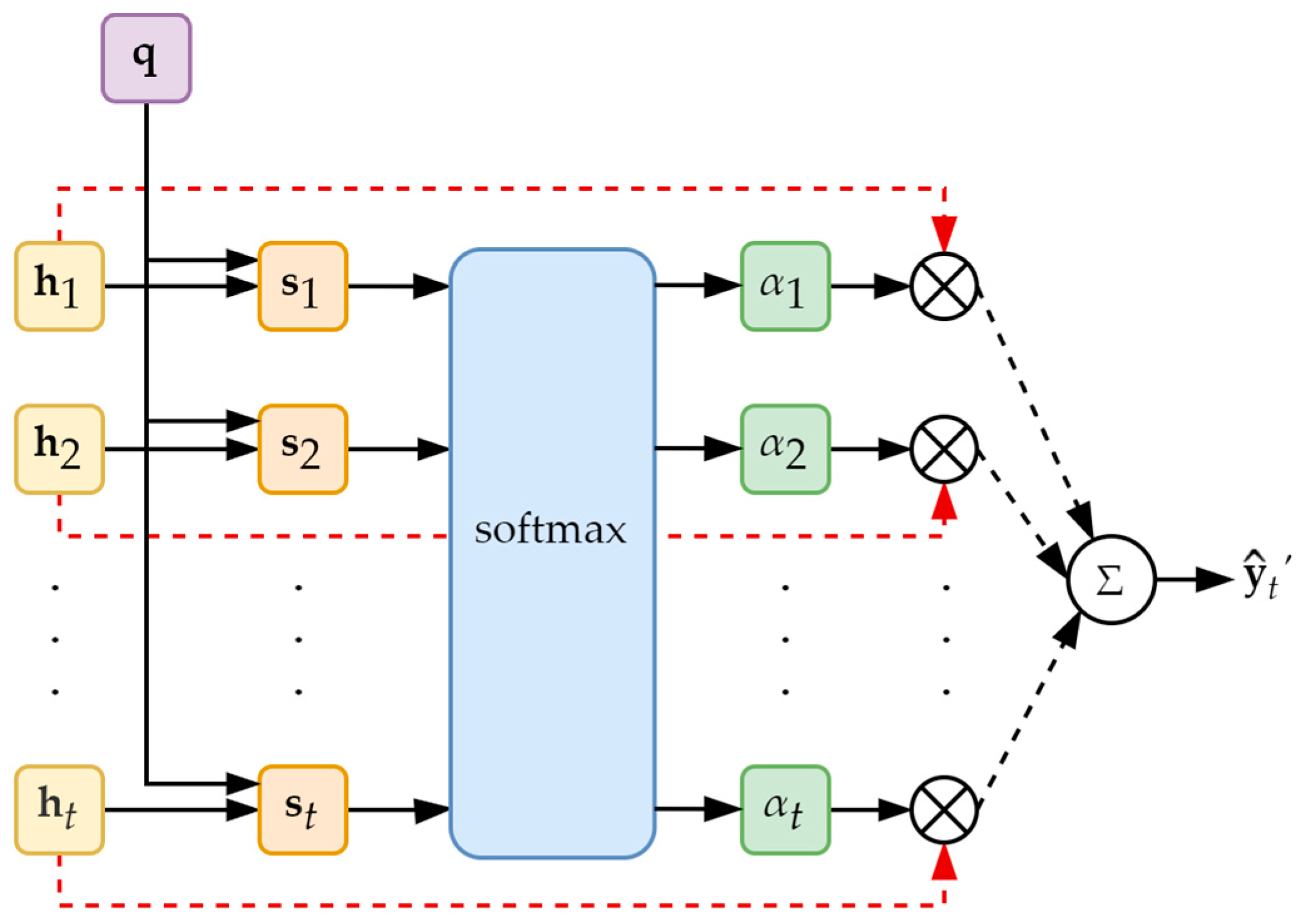
The attention mechanism is a bionic mechanism in deep learning, whose essence is to give more weight to the parts that need to be focused on [35]. The essential idea of the attention mechanism is shown in Figure 3.
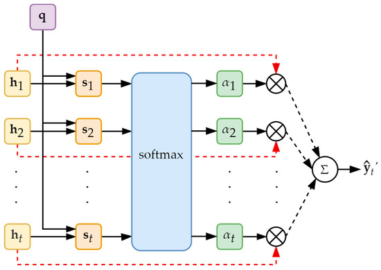
Figure 3.
The attention mechanism.
The calculation of the attention mechanism can be divided into two steps. First, the degree of correlation between the state output of the hidden layer of the LSTM layer and the query vector is calculated using the attention score function , and the corresponding attention weight is obtained using the softmax function. Second, the output of the attention layer is obtained by weighted summation based on the attention weights. The steps are given by
where is the number of time steps.
Then, input into the regression layer to get the predicted tool wear at the current time.
3. Predicting Model
3.1. ConvLSTM-Att Model Construction
According to Zhou et al. [36], the most frequently used sensors in the study of milling process sensor configurations are force, vibration, and acoustic sensors. Therefore, in this paper, the cutting force and vibration along the -, -, and -axes, and the acoustic emission at time , , being the tap index, are selected as the inputs of the model for training the ConvLSTM-Att model, , .
A one-dimensional CNN is first used to extract the high-dimensional features in the measured time-domain data through multiple convolutional layers. The weights of the CNN are updated by backpropagating the error calculated by the loss function. As the number of network layers increases, the problem of the vanishing gradient becomes increasingly obvious. To reduce the impact of vanishing gradients, each convolutional layer is followed by a connection layer, which includes batch normalization, ReLU, and max-pooling layers. The structure is shown in Figure 4.

Figure 4.
A connection layer following each convolutional layer.
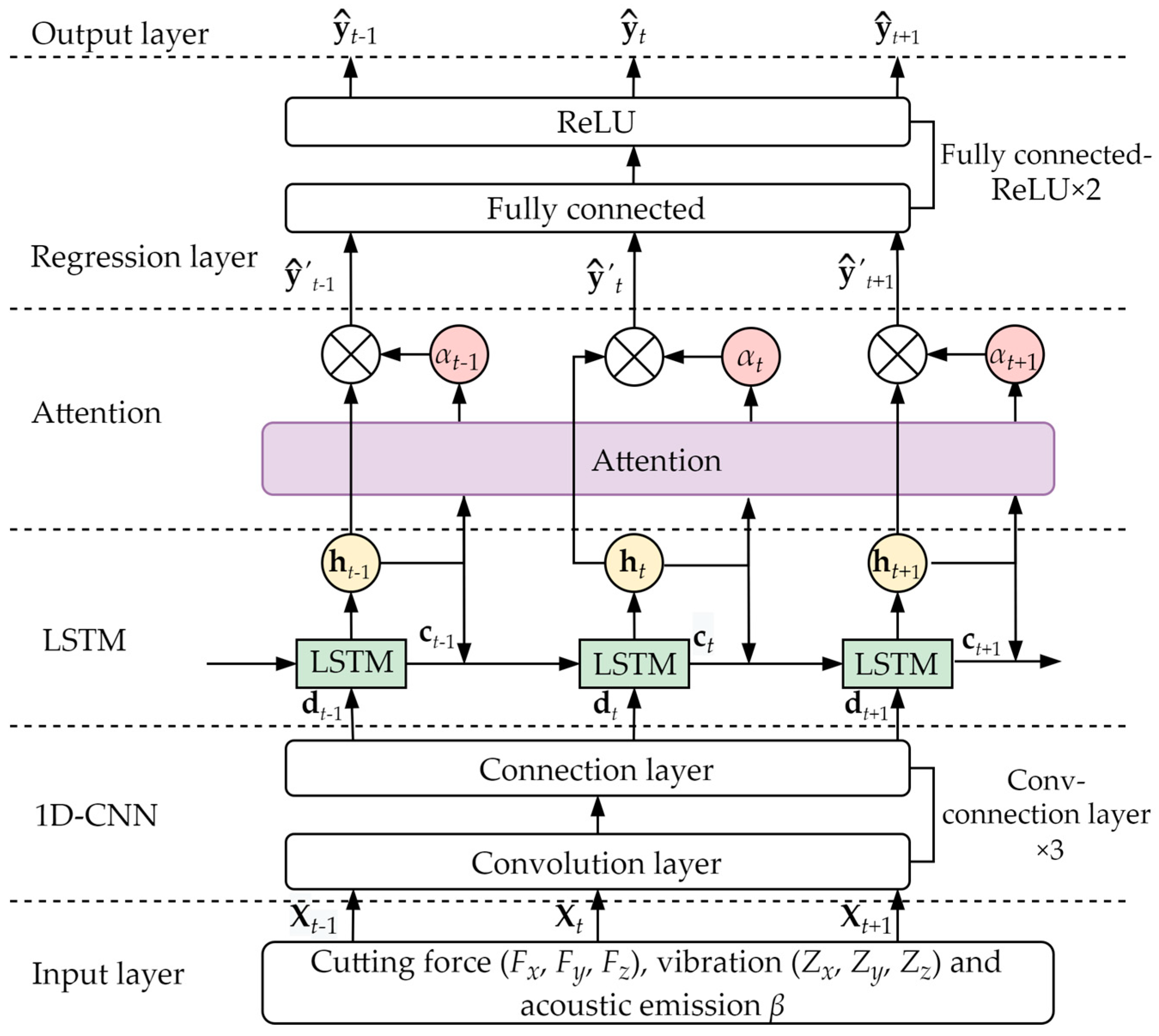
As shown in Figure 5, the ConvLSTM-Att model first automatically mines the features in the tool wear data through the 1D-CNN layer and uses them as the input of the LSTM layer. Then, through the LSTM layer, it learns the temporal relationship between the multidimensional vectors and gets the corresponding hidden layer state vector . Finally, through the attention layer, the attention weight of each input is calculated, and the predicted tool wear is obtained through the nonlinear regression layer.
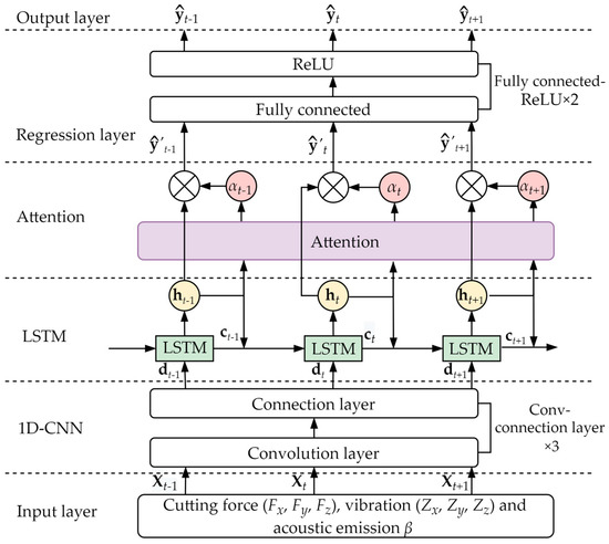
Figure 5.
ConvLSTM-Att model.
3.2. The ConvLSTM-Att Model for Predicting the Tool Wear Process
All data are first normalized and processed, and then divided into different data sets. Train the ConvLSTM-Att model using the training set data. The accuracy of the model is improved by adjusting the model parameters and structure according to the validation results from the validation set. Apply the optimal ConvLSTM-Att model to the test set and output the predicted wear to evaluate the model’s performance. The specific operations are given in Algorithm 1.
| Algorithm 1. Training of the ConvLSTM-Att model |
| Input: Tool wear data set , learning rate , epoch , LSTM neuron number , maximum error . 1. All data are processed by max-min normalization. 2. Divide into the training set , validation set and test set . 3. Perform training with : do Adjust , , , . Train ConvLSTM-Att model with . Validate the currently trained model using . while ( does not converges && ) return the current training model. End 4. Applying the optimal model to . |
| Output: for |
The loss function of the model is the mean square error (MSE) function,
where is the predicted wear and is the measured wear.
The accuracy indices are the mean absolute error (MAE), root mean square error (RMSE) and coefficient of determination R2, given by
where is the average of all measured wear.
4. Experimental Study and Results
4.1. Experimental Setting
The proposed method was validated using the tool wear data set published by the PHM Association in 2010 [37]. The experimental parameters are shown in Table 1.

Table 1.
Experimental parameters.
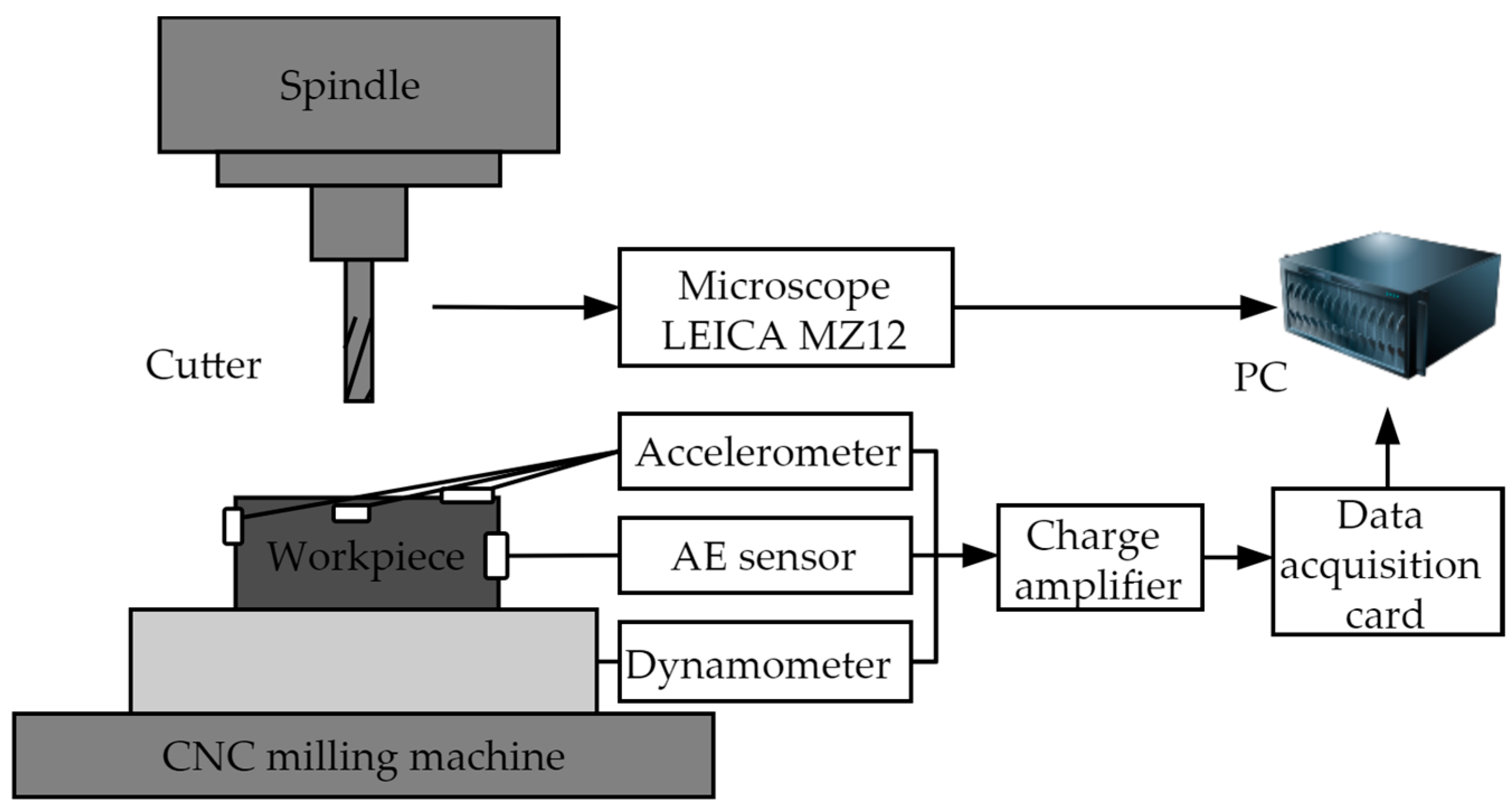
The tool used for the experiments was a three-tooth end mill, and the material machined was HRC52 stainless steel. The experiments were conducted at room temperature with dry cutting—that is, no cutting fluid was used. The force and vibration data in the -, - and -axes during each machining process and the acoustic emission data during the tool move process were collected using a Kistler force gauge, an acceleration sensor, and an acoustic emission sensor, respectively. During each machining process, the tool cut in the x-direction had a length of 108 mm. After each tool move, the wear of the rear face of each tool cutter flute was measured with a LEICA MZ12 microscope to get the wear of each tool move. The sensor setup is shown in Figure 6.

Figure 6.
Experimental setup.
A total of three tools (C1, C4, and C6) were used to collect data for the experiments, each acquiring 315 samples for a total of 945 samples. Each sample contains seven components: cutting force , vibration , acoustic emission as input, and the wear of three cutter flutes as output. According to the recommendations of ISO 8688-2 (1989), the average of the wears of the three cutter flutes was taken as the measured wear of that sample, which was used as the output in the data set. Take the tool C1 as an example, as shown in Figure 7. According to the trend of tool wear, 0~50 tool moves (wear < 90 μm) were classified as the initial wear stage, 51~190 tool moves (wear < 120 μm) as the normal wear stage, and 191~315 tool moves (wear < 173 μm) as the severe wear stage.
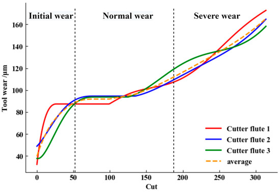
Figure 7.
Division of tool wear stages.
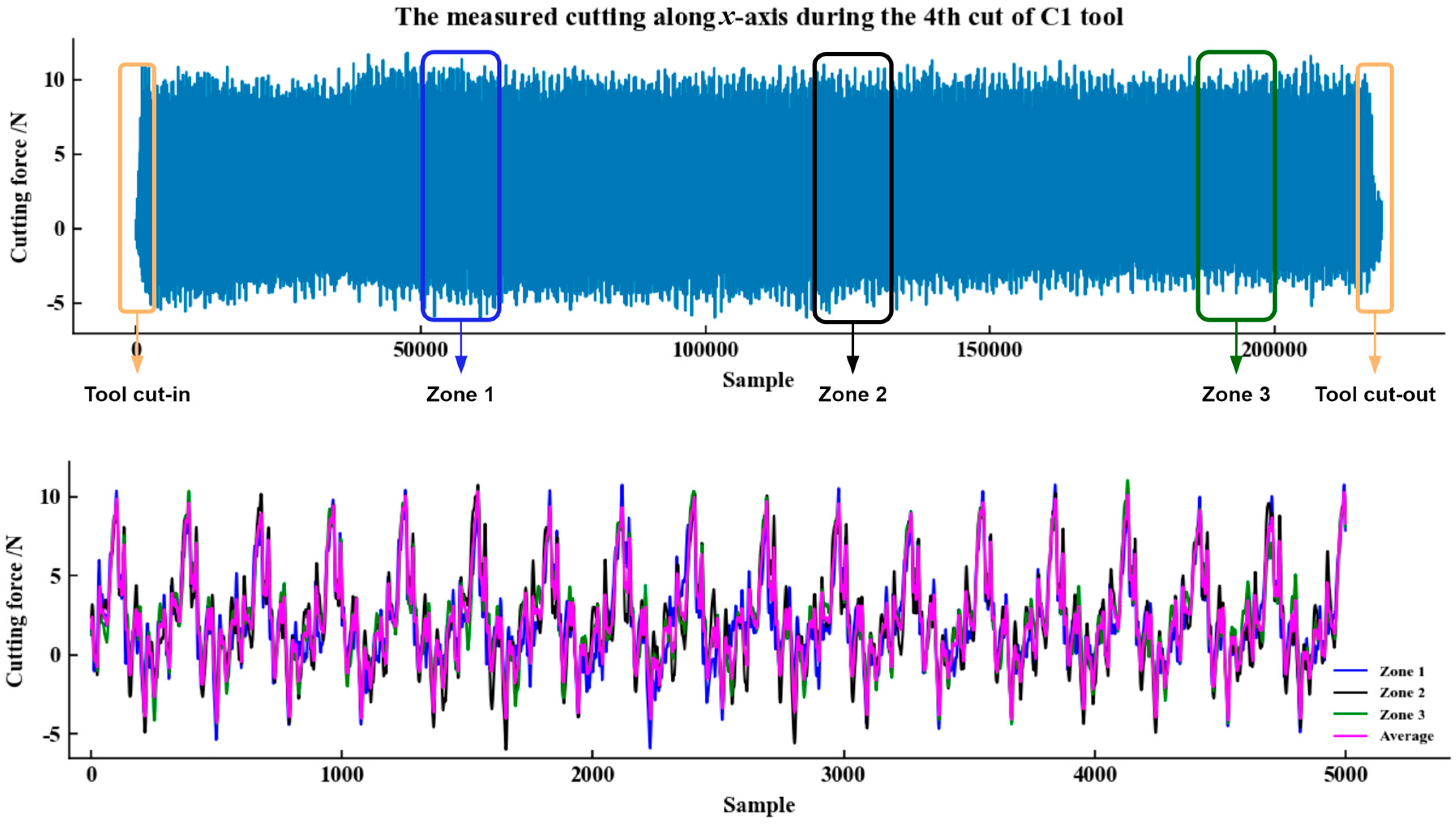
The experiments were conducted at a sampling frequency of 50 kHz, resulting in up to 200,000 data points per sample. In order to exclude the interference of the incoming and outgoing cutters and simplify the computation, three segments of 5000 data-points were selected, as shown in Figure 8. It can be seen from Figure 8 that the maximum and minimum values of the data in each segment are similar. In order to retain the data characteristics of each segment, the average value of the three segments was taken as the model input for training, so that each wear corresponded to tool wear data with a size of 5000 × 7. In order to obtain a reliable and stable model, cross validation was used, and data sets were divided. Among the C1, C4, and C6 data sets, two of the data sets are divided into a training set and a validation set for model training and model parameter adjustment. The ratio of the training set to the verification set is 8:2. The third data set was used as a test set for model evaluation.
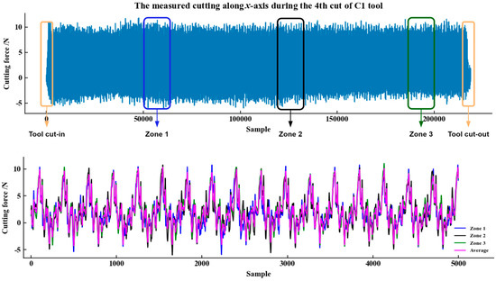
Figure 8.
A close-up of the measured data.
The model is built with the PyTorch deep learning library. It is coded in python and runs on Python 3.7, CUDA 11.4, and Windows with an Intel Core i7 CPU and an NVIDIA GeForce Mx350 GPU.
4.2. Experimental Design and Parameter Setting
In order to verify the accuracy as well as the effectiveness of the tool wear prediction based on the proposed ConvLSTM-Att model, experiments were conducted using the same CNN, CNN-LSTM, and ConvLSTM-Att data set.
In the convolutional model, a small convolutional kernel can reduce the complexity of the model computation, and a small convolutional step size can improve the accuracy of the feature extraction results. Therefore, the size of the convolution kernel is set to (3, 7), the step length is set to 2, and the boundary fill is 1. To avoid losing too many features in the downscaling process, the pooling layer is selected as max-pooling, and the pooling size is set (4, 4). The number of epochs is 500, the initial parameter of the learning rate is 0.001, which decays as the epoch increases, and the optimizer is Adam. To improve the robustness and generalization ability of the model, a dropout layer is added to the regression layer, and the retention rate is set to 0.5. The number of LSTM hidden layer neurons is 128. The maximum error is 6.3.
4.3. Comparison and Analysis of Experimental Results
The models are trained on the training set, the trained model parameters are adjusted on the validation set, and the models are evaluated on the test set. For each model, RMSE, MAE, and R2 are calculated on each test set separately. If the error is large, it means that the model is not properly fitted, and we need to readjust the parameters or train the model structure. The smaller the error, the higher the accuracy of the model. The prediction errors of tool wear for different models on different test sets are shown in Table 2. The calculation times of the 1D-CNN, CNN-LSTM, and ConvLSTM-Att models are shown in Table 3. The performance results of different models for tool wear prediction on different test sets are shown in Figure 9, Figure 10 and Figure 11.

Table 2.
Error performance of different models on different test sets.

Table 3.
The calculation time of the 1D-CNN, CNN-LSTM and ConvL-Att models.

Figure 9.
Predicted results of 1D-CNN model on the C1, C4 and C6 test sets.

Figure 10.
Predicted results of CNN-LSTM model on the C1, C4 and C6 test sets.

Figure 11.
Predicted results of ConvLSTM-Att model on the C1, C4 and C6 test sets.
It can be seen that the 1D-CNN model has the worst overall performance, which is shown in Figure 9. The model-fitting results are poor, and the predicted results of this model at the initial and severe wear stages of the tool have a large gap with the measured wear, which leads to model errors that are generally large. Then, as shown in Figure 10, the accuracy of the CNN-LSTM model is substantially improved compared with that of the 1D-CNN model, and the predicted wear of the model basically fits the measured wear. Due to the fact that the measured time-domain data of tool wear are essentially sequential data, adding the learning of temporal features to the 1D-CNN can improve the accuracy of the model’s prediction. However, there is still a large error in predicting the wear at the initial and severe wear stages of the tool, especially at the severe wear stage for tool C6. From Figure 11, the tool wear predicted using the ConvLSTM-Att model is closer to the measured one. The model improves the ability to extract the key features of tool wear and thus has achieved a higher level of accuracy in predicting the normal and severe wear stages of the tool. Although the prediction of the initial tool wear phase still has some errors, it has been improved compared to the CNN-LSTM model.
From Table 3, the CNN-LSTM model has a complexity that is slightly higher than 1D-CNN and CNN-LSTM due to the extra structural components in the model. Its complexity is higher than 1D-CNN and CNN-LSTM by 91.6% and 14.8%, respectively. RNN and 1D-CNN models have similar complexity, but the 1D-CNN model has better prediction accuracy. The CNN-LSTM and TDconvLSTM models have similar complexity and prediction accuracy. Compared with the CNN-LSTM model, the ConvLSTM-Att model has similar complexity but better prediction accuracy.
On the three different test sets, the ConvLSTM-Att model reduced the RMSE by 60.8%, 67.4%, and 63.7%, and the MAE by 61.7%, 71.3%, and 68.8%, respectively, compared with the 1D-CNN model. When compared with the CNN-LSTM model, the RMSE was reduced by 34.4%, 37.1%, and 46.3%, respectively, and the MAE decreased by 39.6%, 37.6%, and 47.7%, respectively. The results of the ConvLSTM-Att model are also compared with several state-of-the-art models using the same data sets, as shown in Table 2. Compared with these models, the ConvLSTM-Att model has the smallest RMSE and MAE in predicting tool wear, which further confirms the effectiveness and superiority of the ConvLSTM-Att model.
5. Conclusions
In this paper, a tool wear prediction model based on an attentional composite neural network is proposed. Based on a large amount of tool wear data, the original time-domain data in the tool machining state is used as input, and the wear features are mined by 1D-CNN. Using LSTM and attention mechanisms to learn the important tool wear features, the measured wear is approximated by regression. By comparing the predicted tool wear and the measured tool wear, it is confirmed that the ConvLSTM-Att model can well reflect the trend of aggravating tool wear during machining. Under the same test set, the error rate in the tool wear prediction using the ConvLSTM-Att model has decreased significantly compared with other state-of-the-art models. For different test sets, the prediction curves derived from the ConvLSTM-Att model can accurately approximate the measured wear. In sum, the ConvLSTM-Att model provides higher prediction accuracy and better generalization ability compared with the existing models.
Author Contributions
Conceptualization, R.L. and X.Y.; methodology, R.L., X.Y. and K.-L.D.; software, X.Y. and F.Y.; validation, X.Y. and F.Y.; formal analysis, X.Y.; investigation, X.Y.; resources, R.L. and X.Y.; data curation, X.Y. and F.Y.; writing—original draft preparation, X.Y.; writing—review and editing, R.L. and K.-L.D.; visualization, X.Y. and F.Y.; supervision, R.L. and K.-L.D.; project administration, R.L.; funding acquisition, R.L. and K.-L.D. All authors have read and agreed to the published version of the manuscript.
Funding
This work was funded in part by the Zhejiang Provincial 2023 Annual Leading Research and Development Program under Grant no. 2022C01SA111123 and in part by the National Natural Science Foundation of China under Grant no. 51475434.
Institutional Review Board Statement
Not applicable.
Informed Consent Statement
Not applicable.
Data Availability Statement
PHM Society: 2010 PHM Society Conference Data Challenge. Available online: https://www.phmsociety.org/competition/phm/10.
Conflicts of Interest
The authors declare no conflict of interest.
References
- Salierno, G.; Leonardi, L.; Cabri, G. The Future of Factories: Different Trends. Appl. Sci. 2021, 11, 9980. [Google Scholar] [CrossRef]
- Lu, J.; Chen, R.; Liang, H.; Yan, Q. The Influence of Concentration of Hydroxyl Radical on the Chemical Mechanical Polishing of SiC Wafer Based on the Fenton Reaction. Precis. Eng. 2018, 52, 221–226. [Google Scholar] [CrossRef]
- Chen, N.; Hao, B.; Guo, Y.; Li, L.; Khan, M.A.; He, N. Research on Tool Wear Monitoring in Drilling Process Based on APSO-LS-SVM Approach. Int. J. Adv. Manuf. Technol. 2020, 108, 2091–2101. [Google Scholar] [CrossRef]
- Yang, X.; Yuan, R.; Lv, Y.; Li, L.; Song, H. A Novel Multivariate Cutting Force-Based Tool Wear Monitoring Method Using One-Dimensional Convolutional Neural Network. Sensors 2022, 22, 8343. [Google Scholar] [CrossRef]
- García-Ordás, M.T.; Alegre-Gutiérrez, E.; Alaiz-Rodríguez, R.; González-Castro, V. Tool Wear Monitoring Using an Online, Automatic and Low Cost System Based on Local Texture. Mech. Syst. Signal Process. 2018, 112, 98–112. [Google Scholar] [CrossRef]
- Du, K.-L.; Swamy, M.N.S. Neural Networks and Statistical Learning; Springer London: London, UK, 2019; ISBN 978-1-4471-7451-6. [Google Scholar]
- Du, K.-L.; Swamy, M.N.S. Neural Networks in a Softcomputing Framework; Springer-Verlag: London, UK, 2006; ISBN 978-1-84628-302-4. [Google Scholar]
- Du, K.-L.; Swamy, M.N.S. Search and Optimization by Metaheuristics; Springer International Publishing: Cham, Switzerland, 2016; ISBN 978-3-319-41191-0. [Google Scholar]
- Li, J.; Wang, Y.; Du, K.-L. Distribution Path Optimization by an Improved Genetic Algorithm Combined with a Divide-and-Conquer Strategy. Technologies 2022, 10, 81. [Google Scholar] [CrossRef]
- Kuntoğlu, M.; Aslan, A.; Pimenov, D.Y.; Usca, Ü.A.; Salur, E.; Gupta, M.K.; Mikolajczyk, T.; Giasin, K.; Kapłonek, W.; Sharma, S. A Review of Indirect Tool Condition Monitoring Systems and Decision-Making Methods in Turning: Critical Analysis and Trends. Sensors 2020, 21, 108. [Google Scholar] [CrossRef] [PubMed]
- Mao, W.; Feng, W.; Liu, Y.; Zhang, D.; Liang, X. A New Deep Auto-Encoder Method with Fusing Discriminant Information for Bearing Fault Diagnosis. Mech. Syst. Signal Process. 2021, 150, 107233. [Google Scholar] [CrossRef]
- Wang, J.; Xie, J.; Zhao, R.; Zhang, L.; Duan, L. Multisensory Fusion Based Virtual Tool Wear Sensing for Ubiquitous Manufacturing. Robot. Comput.-Integr. Manuf. 2017, 45, 47–58. [Google Scholar] [CrossRef]
- Qiu, J.; Wang, H.; Lu, J.; Zhang, B.; Du, K.-L. Neural Network Implementations for PCA and Its Extensions. ISRN Artif. Intell. 2012, 2012, 847305. [Google Scholar] [CrossRef]
- Feng, T.; Guo, L.; Gao, H.; Chen, T.; Yu, Y.; Li, C. A New Time–Space Attention Mechanism Driven Multi-Feature Fusion Method for Tool Wear Monitoring. Int. J. Adv. Manuf. Technol. 2022, 120, 5633–5648. [Google Scholar] [CrossRef]
- Zhao, R.; Yan, R.; Chen, Z.; Mao, K.; Wang, P.; Gao, R.X. Deep Learning and Its Applications to Machine Health Monitoring. Mech. Syst. Signal Process. 2019, 115, 213–237. [Google Scholar] [CrossRef]
- Voulodimos, A.; Doulamis, N.; Doulamis, A.; Protopapadakis, E. Deep Learning for Computer Vision: A Brief Review. Comput. Intell. Neurosci. 2018, 2018, 7068349. [Google Scholar] [CrossRef]
- Song, Z. English Speech Recognition Based on Deep Learning with Multiple Features. Computing 2020, 102, 663–682. [Google Scholar] [CrossRef]
- Otter, D.W.; Medina, J.R.; Kalita, J.K. A Survey of the Usages of Deep Learning for Natural Language Processing. IEEE Trans. Neural Netw. Learn. Syst. 2021, 32, 604–624. [Google Scholar] [CrossRef]
- Luo, B.; Wang, H.; Liu, H.; Li, B.; Peng, F. Early Fault Detection of Machine Tools Based on Deep Learning and Dynamic Identification. IEEE Trans. Ind. Electron. 2019, 66, 509–518. [Google Scholar] [CrossRef]
- Kothuru, A.; Nooka, S.P.; Liu, R. Application of Deep Visualization in CNN-Based Tool Condition Monitoring for End Milling. Procedia Manuf. 2019, 34, 995–1004. [Google Scholar] [CrossRef]
- Xu, X.; Wang, J.; Ming, W.; Chen, M.; An, Q. In-Process Tap Tool Wear Monitoring and Prediction Using a Novel Model Based on Deep Learning. Int. J. Adv. Manuf. Technol. 2021, 112, 453–466. [Google Scholar] [CrossRef]
- Chen, Q.; Xie, Q.; Yuan, Q.; Huang, H.; Li, Y. Research on a Real-Time Monitoring Method for the Wear State of a Tool Based on a Convolutional Bidirectional LSTM Model. Symmetry 2019, 11, 1233. [Google Scholar] [CrossRef]
- Zhao, R.; Wang, J.; Yan, R.; Mao, K. Machine Health Monitoring with LSTM Networks. In Proceedings of the 2016 10th International Conference on Sensing Technology (ICST), Nanjing, China, 11–13 November 2016; pp. 1–6. [Google Scholar]
- Cai, W.; Zhang, W.; Hu, X.; Liu, Y. A Hybrid Information Model Based on Long Short-Term Memory Network for Tool Condition Monitoring. J. Intell. Manuf. 2020, 31, 1497–1510. [Google Scholar] [CrossRef]
- Chan, Y.-W.; Kang, T.-C.; Yang, C.-T.; Chang, C.-H.; Huang, S.-M.; Tsai, Y.-T. Tool Wear Prediction Using Convolutional Bidirectional LSTM Networks. J. Supercomput. 2022, 78, 810–832. [Google Scholar] [CrossRef]
- Schwendemann, S.; Sikora, A. Transfer-Learning-Based Estimation of the Remaining Useful Life of Heterogeneous Bearing Types Using Low-Frequency Accelerometers. J. Imaging 2023, 9, 34. [Google Scholar] [CrossRef]
- Qiao, H.; Wang, T.; Wang, P. A Tool Wear Monitoring and Prediction System Based on Multiscale Deep Learning Models and Fog Computing. Int. J. Adv. Manuf. Technol. 2020, 108, 2367–2384. [Google Scholar] [CrossRef]
- Wang, G.; Zhang, F. A Sequence-to-Sequence Model With Attention and Monotonicity Loss for Tool Wear Monitoring and Prediction. IEEE Trans. Instrum. Meas. 2021, 70, 1–11. [Google Scholar] [CrossRef]
- Huang, Q.; Wu, D.; Huang, H.; Zhang, Y.; Han, Y. Tool Wear Prediction Based on a Multi-Scale Convolutional Neural Network with Attention Fusion. Information 2022, 13, 504. [Google Scholar] [CrossRef]
- Li, Z.; Liu, F.; Yang, W.; Peng, S.; Zhou, J. A Survey of Convolutional Neural Networks: Analysis, Applications, and Prospects. IEEE Trans. Neural Netw. Learn. Syst. 2022, 33, 6999–7019. [Google Scholar] [CrossRef]
- Huang, Z.; Zhu, J.; Lei, J.; Li, X.; Tian, F. Tool Wear Predicting Based on Multi-Domain Feature Fusion by Deep Convolutional Neural Network in Milling Operations. J. Intell. Manuf. 2020, 31, 953–966. [Google Scholar] [CrossRef]
- Kiranyaz, S.; Avci, O.; Abdeljaber, O.; Ince, T.; Gabbouj, M.; Inman, D.J. 1D Convolutional Neural Networks and Applications: A Survey. Mech. Syst. Signal Process. 2021, 151, 107398. [Google Scholar] [CrossRef]
- Van Houdt, G.; Mosquera, C.; Nápoles, G. A Review on the Long Short-Term Memory Model. Artif. Intell. Rev. 2020, 53, 5929–5955. [Google Scholar] [CrossRef]
- Sherstinsky, A. Fundamentals of Recurrent Neural Network (RNN) and Long Short-Term Memory (LSTM) Network. Phys. D Nonlinear Phenom. 2020, 404, 132306. [Google Scholar] [CrossRef]
- Niu, Z.; Zhong, G.; Yu, H. A Review on the Attention Mechanism of Deep Learning. Neurocomputing 2021, 452, 48–62. [Google Scholar] [CrossRef]
- Zhou, Y.; Xue, W. Review of Tool Condition Monitoring Methods in Milling Processes. Int. J. Adv. Manuf. Technol. 2018, 96, 2509–2523. [Google Scholar] [CrossRef]
- PHM Society: 2010 PHM Society Conference Data Challenge. Available online: https://www.phmsociety.org/competition/phm/10 (accessed on 13 January 2023).
- Qiao, H.; Wang, T.; Wang, P.; Qiao, S.; Zhang, L. A Time-Distributed Spatiotemporal Feature Learning Method for Machine Health Monitoring with Multi-Sensor Time Series. Sensors 2018, 18, 2932. [Google Scholar] [CrossRef]
Disclaimer/Publisher’s Note: The statements, opinions and data contained in all publications are solely those of the individual author(s) and contributor(s) and not of MDPI and/or the editor(s). MDPI and/or the editor(s) disclaim responsibility for any injury to people or property resulting from any ideas, methods, instructions or products referred to in the content. |
© 2023 by the authors. Licensee MDPI, Basel, Switzerland. This article is an open access article distributed under the terms and conditions of the Creative Commons Attribution (CC BY) license (https://creativecommons.org/licenses/by/4.0/).

