Abstract
Intelligent lower-limb prosthesis appears in the public view due to its attractive and potential functions, which can help amputees restore mobility and return to normal life. To realize the natural transition of locomotion modes, locomotion mode classification is the top priority. There are mainly five steady-state and periodic motions, including LW (level walking), SA (stair ascent), SD (stair descent), RA (ramp ascent), and RD (ramp descent), while ST (standing) can also be regarded as one locomotion mode (at the start or end of walking). This paper mainly proposes four novel features, including TPDS (thigh phase diagram shape), KAT (knee angle trajectory), CPO (center position offset) and GRFPV (ground reaction force peak value) and designs ST classifier and artificial neural network (ANN) classifier by using a user-dependent dataset to classify six locomotion modes. Gaussian distributions are applied in those features to simulate the uncertainty and change of human gaits. An angular velocity threshold and GRFPV feature are used in the ST classifier, and the artificial neural network (ANN) classifier explores the mapping relation between our features and the locomotion modes. The results show that the proposed method can reach a high accuracy of 99.16% ± 0.38%. The proposed method can provide accurate motion intent of amputees to the controller and greatly improve the safety performance of intelligent lower-limb prostheses. The simple structure of ANN applied in this paper makes adaptive online learning algorithms possible in the future.
1. Introduction
According to the statistics of the World Health Organization (WHO), about 15% (975 million) of the world’s population have physical disabilities to varying degrees [1]. Some of them suffer from lower-limb amputation (LLA). For people with LLA, lower limb prosthesis is an important tool to help them restore mobility and live a better life. However, at present, the majority of commercial prosthetic legs are passive, and walking with them will consume 20~30% more energy than healthy individuals [2]. Moreover, the obvious asymmetry between the sound side and the affected side will lead to secondary damage. When people with LLA are in a complex walking environment, even stability will become a luxury [3]. Research on intelligent lower-limb prostheses has been performed recently due to their adaptation in different terrains.
The common control framework of intelligent lower-limb prostheses is a hierarchical control system [4] shown in Figure 1. The high-level controller focuses on human intent recognition to distinguish locomotion modes in real time and obtain gait parameters and gait phase, which will be sent to the middle-level controller to compute desired joint angles and torques. The low-level controller aims at making the actuators output the desired torques. In this paper, we focus on locomotion mode classification, which belongs to the high-level controller of the prosthesis control system.
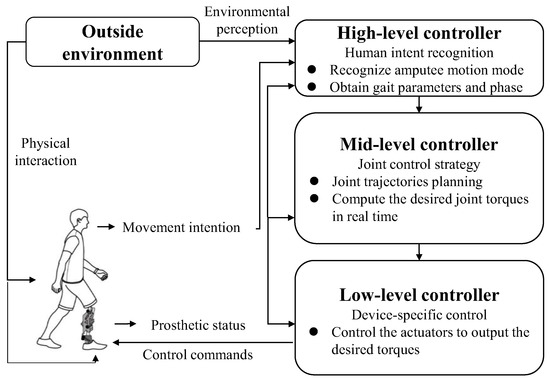
Figure 1.
The hierarchical control system [4] of intelligent powered low limb prosthesis based on the gait phase.
Pattern recognition (PR), machine learning (ML), and statistical methods have been widely applied to classify locomotion modes from surface electromyogram (sEMG) signals [5] to mechanical sensors. Ref. [6] collects sEMG signals to interpret motion modes. J A Spanias et al. developed an adaptive PR system to adapt to changes in the user’s neural information during ambulation and consistently identify the user’s intent over multiple days with a classification accuracy of 96.31% ± 0.91% [7]. Zhang et al. present a robust environmental feature recognition system (EFRS) to predict the locomotion modes of amputees and estimate environmental features with the depth camera [8]. Ref. [9] combines EMG and mechanical sensors, using linear discriminant analysis (LDA) to reach 86% accuracy. Quadratic discriminant analysis (QDA) in [10] gets a similar result with EMG only. Ref. [11] infers the user’s intent with the Gaussian mixture model (GMM). They combine foot force and EMG to distinguish intent to stand, sit and walk. Ref. [12] combines all sensors to recognize six locomotion modes and five mode transitions by support vector machine (SVM) and gets a high accuracy of 95%. Ref. [13] adopts dynamic Bayesian network (DBN) to recognize level walking (LW), stair ascent (SA), stair descent (SD), ramp ascent (RA) and ramp descent (RD) with a load cell and a six-axis inertial measurement unit (IMU). Ref. [14] depends only on ground reaction force (GRF) to distinguish LW and SD by an artificial neural network (ANN). Recently, [15] encodes data from IMUs into picture format and inputs this 2D image into a convolutional neural network (CNN). The CNN outputs the probability of five steady states and eight transition states. They successfully improve the accuracy to 95.8%. Similarly, Kang et al. developed a DL-based (deep learning-based) classifier for five steady states, which is user-independent and achieved an overall accuracy of 98.84% ± 0.47% [16]. Ref. [17] uses ML methods to compare the user-independent and dependent intent recognition systems for powered prostheses. The results show that the user-dependent method has better accuracy. The previous works have achieved good results in locomotion mode classification. However, the traditional extracted features are generally the average, maximum, minimum, median and variance of sensors’ data, which lack a physical explanation. The DL methods need big data collection, which is unfriendly to the amputees.
Based on 2 IMUs (Placed on the thigh and shank of amputees’ sound leg, respectively) and a GRF insole (Placed in the amputees’ sound leg’s shoe), shown in Figure 2, which are used to collect a user-dependent dataset, this paper extracts four novel features and design classifiers to recognize locomotion modes. The main contributions of this paper are as follows: (1) based on the processed sensor data, four novel features are extracted; (2) the fluctuation of gait data is expressed by Gaussian distributions to simulate the fluctuation of human motion trajectory; (3) The designed classifiers achieve a higher accuracy of 99.16% ± 0.38% compared with previous works.
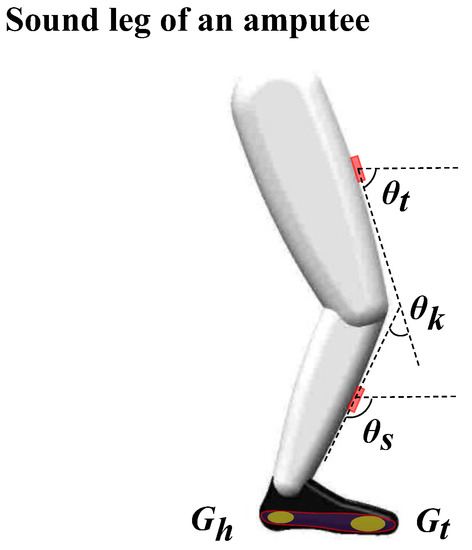
Figure 2.
Sensor installation positions and variable descriptions. is the thigh IMU angle in the sagittal plane, is the shank IMU angle in the sagittal plane and is the knee angle. and are the raw force sensor data of the heel and toe.
2. Materials and Methods
2.1. Data Acquisition and Processing
2.1.1. Data Collection
Eight able-bodied subjects agreed to participate in the data acquisition experiments, including six males (varies in height (1.63–1.81 m) and weight (58–76 kg)) and two females (varies in height (1.65–1.7 m) and weight (50–55 kg)). They are required to equip with an intelligent prosthesis in Figure 3a. The intelligent lower-limb prosthesis is designed for healthy individuals in which the knee and ankle are active joints that provide power in the sagittal plane. The finite state machine impedance control [18] is applied for the intelligent prosthesis, and the joint torques are determined according to Equation (1)
where denotes the prosthesis knee or ankle, is the joint angle and is the joint angular velocity. , and are the stiffness, damping and equilibrium positions, respectively, and are assigned different values under different states and locomotion modes. The impedance parameters are set to make the subject walk comfortably.
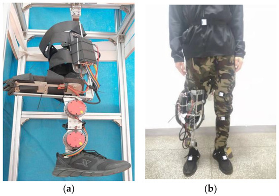
Figure 3.
(a) Intelligent lower-limb prosthesis designed for able-bodied subjects. (b) The able-bodied subject equipped with a prosthesis and data acquisition sensors.
Moreover, data acquisition sensors, including IMUs and GRF insoles, are set, as shown in Figure 3b. IMU data consist of angle and angular velocity in the x, y, and z-axis directions, respectively, with a sampling frequency of 100 Hz. The GRF insoles measure pressure in the vertical direction with a frequency of 100 Hz.
This paper aims to classify 6 locomotion modes, shown in Figure 4, and the locomotion settings, including an incline-adjustable treadmill and 2 stairs of different heights, are shown in Figure 5. The ramp inclines are set to ±3.6°, ±5.8° and ±9.5°. Under each incline, subjects walk for 30 s with low, normal and fast speeds (0.56 m/s, 0.83 m/s and 1.11 m/s). To keep the data sizes in different modes almost the same, each subject walks on the level ground (LG) for 90 s at each speed. As for SA and SD, subjects completed 10 trials under different stair heights of 11.8 cm and 14.5 cm. Finally, subjects maintain a relaxing standing posture on level ground for 60 s.
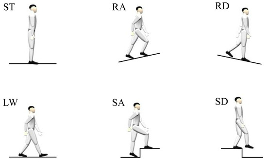
Figure 4.
Six locomotion modes including level walking (LW), stair ascent (SA), stair descent (SD), ramp ascent (RA), ramp descent (RD), and standing (ST).
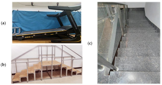
Figure 5.
(a) Incline adjustable treadmill. (b) Stairs with 14.5 cm stair height. (c) Stairs with 11.8 cm stair height.
Our final dataset includes data from 3 sensors: 2 IMUs placed at the thigh and the shank of the sound leg and a GRF insole put in the shoe on the same side (Figure 2). We only used IMU data in the sagittal plane direction. The raw sensor dataset under mode is recorded as follows:
For clarity, we list some parameters in Table 1 below and some abbreviations in Table A1 of Appendix A.

Table 1.
Variable descriptions.
2.1.2. Gait Phase Variable
There are experiments using motion capture systems that prove that the human thigh motion can uniquely and continuously represent the gait cycle [19]. The continuous gait phase variable is defined by the atan2 function:
However, there are noises and ground impact in thigh angular velocity . The linear polynomial fitting method is adopted to smooth the curve, as shown in Figure 6a.
where and are linear fitting parameters calculated by the least square method online according to Equation (5), and is the smoothing coefficient. In Equation (5), is the sample number. Here, and .
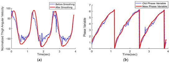
Figure 6.
(a) Smoothing effect on the normalized thigh Angular velocity. (b) The new gait phase variable shows better monotonicity at the time axis.
By translation, the phase diagram trajectory can wrap the origin and make the phase variable vary circularly. By normalization, we can obtain a similar phase diagram trajectory under the same locomotion mode with different walking speeds. The transformation formulas [19] are as follows:
where is the scale factor, is the normalization factor, and is the translation factor which can be calculated by:
Data of the previous gait cycle from moment are taken to calculate the maximum and minimum in real time. The new continuous gait phase variable (Figure 6b) is defined as
2.1.3. Knee Angle and GRF value
The knee angle is calculated as:
The smoothing method in Equation (4) ( and ) is applied at the knee angle to get a smoother curve . To obtain similar knee trajectory under the same locomotion mode with different walking speeds, is normalized to .
The GRF of the heel and toe are recorded as and respectively. Their latest peak values are recorded as and during one gait cycle before.
Then, the processed dataset is
is discretized into parts of the same length according to Equation (11).
is divided into according to which part belongs to. The divided datasets are used to calculate feature distributions under different modes. The workflow of offline data processing and feature distribution calculation are shown in Figure 7.
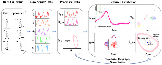
Figure 7.
Offline data processing and feature distribution calculation.
2.2. Feature Distributions and Extractions
2.2.1. Thigh Phase Diagram Shape (TPDS)
The thigh phase diagram consists of processed thigh IMU angle in the x-axis and processed thigh IMU angular velocity in y-axis. The trajectory of during walking is named TDPS, and TDPS varies from each other under different locomotion modes. Here, Gaussian distributions are used to record the standard TDPS of different locomotion modes. For example, the TPDS under LW mode is shown in Figure 8a.
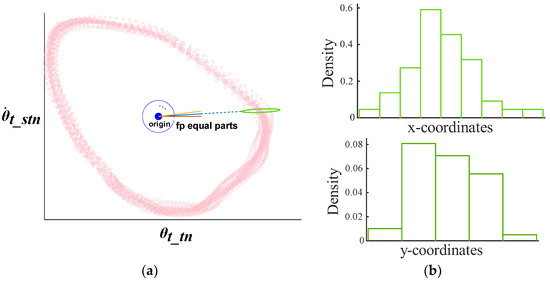
Figure 8.
(a) TPDS of LW mode. Pink points belong to the dataset . Points in the green circle are in the dataset . (b) The distributions of x-coordinates and y-coordinates of points in the green circle are near to normal according to the histograms.
From Figure 8b, it is known that correspond to a two-dimensional Gaussian distribution . For each , it can be calculated as:
Gaussian distributions from to together represent the TPDS under mode. TPDSs in different locomotion modes are shown in Figure 9a.
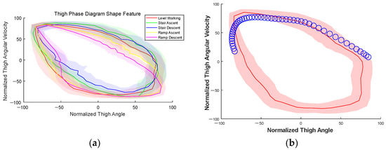
Figure 9.
(a) TPDSs in different locomotion modes. The solid line is the mean trajectory, and the transparent area is ±1 standard deviation. (b) The red part is the standard TPDS of LW mode. Blue points form the real-time thigh phase diagram trajectory, and the blue points are collected under LW mode.
The overlap degree between real-time thigh phase diagram trajectory and standard TPDSs of different modes shown in Figure 9b is an index of similarity to classify locomotion modes. The summation of the probability density of each sample point is used to evaluate the overlap degree:
where is the probability density function of . Then we can figure out the conditional probability, of each mode:
where represents the TPDS feature at time .
2.2.2. Knee Angle Trajectory (KAT)
KAT is the normalized knee angle trajectory at the gait phase axis. Similarly to TPDS, correspond to a one-dimensional normal distribution . Standard KATs in different locomotion modes are shown in Figure 10.
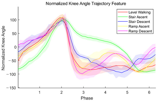
Figure 10.
KATs in different locomotion modes. The x-axis is the continuous thigh phase variable which represents a whole gait cycle, and the y-axis is the normalized knee angle . The solid line is the mean trajectory, and the transparent area is ±1 standard deviation.
The summation of probability density is used to evaluate the overlap degree of real-time KAT and the standard KAT under mode:
where is the probability density function of . The conditional probability of each mode is:
where represents the KAT feature at time .
2.2.3. Center Position Offset (CPO)
During the translation of the thigh phase diagram in Equation (7), the translation vector can reflect the range of thigh motion. The translation vector is called CPO. In different locomotion modes, the distributions of are shown in Figure 11a. The two-dimensional normal distribution function is used to describe CPO under mode. The probability density function of is , and the conditional probability under CPO is
where represents the CPO feature at time .
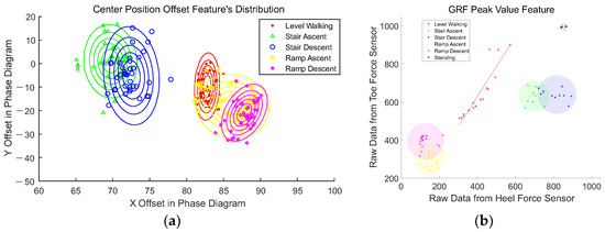
Figure 11.
(a) CPO distributions in different modes. Ellipses represent probability density contours, and the points represent the translation vector in different modes. (b) GRFPV feature distributions in different modes. Points represent parts of sample points . The line segment is fitted by points of . The circles contain all sample points of one mode with the smallest radius.
2.2.4. Ground Reaction Force Peak Value (GRFPV)
The peak values of the force and heel force have different distributions in different locomotion modes, as shown in Figure 11b. We assume that the GRFPV of LW are assembling near a line segment and GRFPV of other modes are gathering in a circle.
The line segment AB is fitted by the least square method:
The coordinate of each circle center of each mode is
Then Euclidean distance is used to compute the relative probability :
where is
where is the GRFPV point in real time. The conditional probability is:
where represents the GRFPV feature at time .
It should be noted that ST is not periodic movement and does not have a stable phase variable. The TPDS, KAT, and CPO features of ST are not calculated.
3. Results
The workflow of real-time feature extraction and classification is shown in Figure 12. This paper designs two classifiers: the standing (ST) classifier is used to identify the ST mode, and the artificial neural network (ANN) classifier is used to classify the other five locomotion modes.

Figure 12.
Real-time feature extraction and classification. C1 is the standing (ST) classifier, and C2 is the artificial neural network (ANN) classifier. The blue points are real-time feature points under LW.
3.1. ST Classifier
An angular velocity threshold and GRFPV feature are used at the ST classifier, as shown in Figure 12. The threshold satisfies
where is the dynamic trend. When the subject is standing, the curve is shown in Figure 13a, and the maximum is smaller than 2. Then, 10,000 sample points are randomly sampled in other modes, and their distribution is shown in Figure 13b. The minimum under other modes is greater than 7. Here, we take .
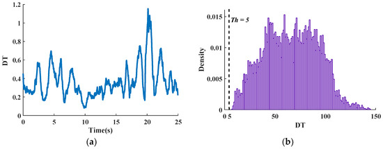
Figure 13.
(a) The dynamic trend under ST mode. (b) Ten thousand sample points are randomly sampled in other modes, and their distribution is shown above.
The threshold ensures that there won’t be much movement, while the GRFPV feature inequality ensures that the subject is standing on the ground. The ST classifier has an accuracy of 100% in the test because standing has an obvious static feature which is different from periodic locomotion modes.
3.2. ANN Classifier
At the ANN classifier, the conditional probabilities of each mode under each feature are input into a fully connected neural network with one hidden layer, as shown in Figure 14, and the final outputs are the probabilities of each locomotion mode. The calculations of the hidden layer and output layer are shown in Equation (24).
where and are the weight matrix and bias between input and hidden layer. and are the weight matrix and bias between the hidden and output layers. is the tansig function. During the training process, the training dataset and validation dataset are strictly separated.
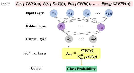
Figure 14.
The structure of the designed neural network.
The data was trained on a particular subject, and the ANN classifier was evaluated by a five-fold cross-validation. The testing results of eight subjects are listed in Table 2 below, and the confusion matrix of eight subjects is shown in Table 3. The ANN classifier has an average accuracy across all subjects of 99.16% ± 0.38%.

Table 2.
Classification results for 8 Subjects.

Table 3.
The confusion matrix of the accuracy tests.
Compared with the traditional confusion matrix, we add one column of “None” to represent the unclassified mode when
4. Discussion
4.1. Network Hyperparameters
The performance of ANN is closely related to the network structure. Here, the following hyperparameters are considered: (1) the number of neurons in the hidden layer (); (2) the number of groups of training data for each mode () in the training set. affects network structure and may lead to overfitting or underfitting. Based on M1′s user-dependent dataset, tests are carried out under different parameters, and the results are shown in Figure 15a. The bigger corresponds to higher classification accuracy. However, classification accuracy has already reached 95% when , which shows that the proposed method can achieve good results when training with a small amount of data. When and , we get the best classification accuracy of M1.
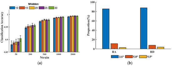
Figure 15.
(a) Classification accuracy under different and . The error bar represents ±1 standard deviation. (b) Error’s proportion of different slopes under RA and RD.
4.2. Ramp Slope
From Table 2 and Table 3, classification errors mainly focus on RA and RD. The proportion of each error of different slopes in the whole error under RA and RD is shown in Figure 15b. The result shows that the main error occurs in the low slopes, which indicates that gaits under low slopes have similarities.
4.3. Time Window Length
Time window size decides how much information we can use when classification is in progress. However, the bigger time window size will bring higher delay. Based on M1′s user-dependent dataset, we test the average accuracy under different time window sizes when and . The result is shown in Figure 16. When the time window size reaches 50, the classification accuracy increases very slowly.
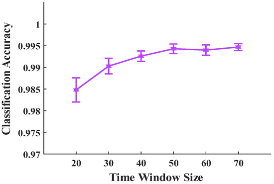
Figure 16.
Classification accuracy under different time window sizes. Error bars represent ±1 standard deviation.
5. Conclusions
The high accuracy of locomotion mode classification ensures prosthetic users’ safety and are the foundation of the natural transition between locomotion modes. In this paper, four novel features are proposed based on data from two IMUs and one GRF insole. Gaussian distributions are used to describe the TPDS, KAT and CPO features after using distribution fitter tools to analyze the data. Euclidean distances in GRFPV diagrams are used to compute the relative probabilities of different locomotion modes. To the author’s knowledge, those features haven’t been proposed and applied yet. ST classifier and ANN classifier are designed and achieve a high accuracy of 100% and 99.16% ± 0.38%, respectively.
Moreover, the proposed method is potential for future research. The real-time classified walking data are used to adjust features’ distribution to adapt amputee’s gaits. The new extracted feature is convenient to be added to our control framework. The ANN used in this paper is simple in structure, which makes it possible to train ANN online. Additionally, human locomotion modes are not limited to the listed. When the predicted class is “None,” we can collect the unclassified data and apply clustering algorithms to discover new modes. Those evolutionary and adaptive abilities are what we will study next.
To further our study, the disabled volunteers will be invited to test the proposed method. Except for locomotion mode classification, more information such as slopes, step stride and stair height will be predicted by analyzing the walking dataset.
Author Contributions
Conceptualization, Y.L. and H.A.; methodology, Y.L. and H.A.; software, Y.L.; validation, Y.L., H.A. and H.M.; formal analysis, Y.L.; data curation, Y.L.; writing—original draft preparation, Y.L.; writing—review and editing, H.A., H.M. and Q.W.; visualization, Y.L.; supervision, H.A., H.M. and Q.W.; project administration, H.A.; funding acquisition, H.A., H.M. and Q.W. All authors have read and agreed to the published version of the manuscript.
Funding
This research was funded by the project of the National Key Research and Development Program of China, grant number (2018YFC2001304).
Informed Consent Statement
Not applicable.
Data Availability Statement
Not applicable.
Conflicts of Interest
The authors declare no conflict of interest.
Appendix A
Abbreviations in this paper are shown in Table A1.

Table A1.
Abbreviations in this paper.
Table A1.
Abbreviations in this paper.
| Abbreviations | Full Names | Abbreviations | Full Names |
|---|---|---|---|
| LW | level walking | SA | stair ascent |
| SD | stair descent | RA | ramp ascent |
| RD | ramp descent | ST | standing |
| TPDS | thigh phase diagram shape | KAT | knee angle trajectory |
| CPO | center position offset | GRFPV | ground reaction force peak value |
| ANN | artificial neural network | WHO | world health organization |
| LLA | lower-limb amputation | PR | pattern recognition |
| ML | machine learning | sEMG | surface electromyogram |
| EFRS | environmental feature recognition system | LDA | linear discriminant analysis |
| QDA | quadratic discriminant analysis | GMM | Gaussian mixture model |
| DBN | dynamic Bayesian network | IMU | inertial measurement unit |
| GRF | ground reaction force | CNN | convolutional neural network |
| DL-based | deep learning based | LG | level ground |
| M | man | W | woman |
| DT | dynamic trend |
References
- Filmer, D. Disability, Poverty, and Schooling in Developing Countries. Soc. Sci. Electron. Publ. Vol. 2008, 22, 141–163. [Google Scholar]
- Au, S.K.; Weber, J.; Herr, H.M. Powered Ankle—Foot Prosthesis Improves Walking Metabolic Economy. IEEE Trans. Robot. 2009, 25, 51–66. [Google Scholar] [CrossRef]
- Wang, Q.N.; Zheng, E.H.; Chen, B.J.; Mai, J.G. Recent Progress and Challenges of Robotic Lower-limb Prostheses for Human-robot Integration. Acta Autom. Sin. 2016, 42, 1780–1793. [Google Scholar]
- Tucker, M.R.; Olivier, J.; Pagel, A.; Bleuler, H.; Bouri, M.; Lambercy, O.; Gassert, R. Control strategies for active lower extremity prosthetics and orthotics: A review. J. NeuroEngineering Rehabil. 2015, 12, 1–30. [Google Scholar] [CrossRef] [PubMed]
- Fleming, A.; Stafford, N.; Huang, S.; Hu, X.; Ferris, D.P.; Huang, H.H. Myoelectric control of robotic lower limb prostheses: A review of electromyography interfaces, control paradigms, challenges and future directions. J. Neural Eng. 2021, 18, 041004. [Google Scholar] [CrossRef] [PubMed]
- Simao, M.; Mendes, N.; Gibaru, O.; Neto, P. A Review on Electromyography Decoding and Pattern Recognition for Human-Machine Interaction. IEEE Access 2019, 7, 39564–39582. [Google Scholar] [CrossRef]
- Spanias, J.A.; Simon, A.M.; Finucane, S.B.; Perreault, E.J.; Hargrove, L.J. Online adaptive neural control of a robotic lower limb prosthesis. J. Neural Eng. 2018, 15, 016015. [Google Scholar] [CrossRef] [PubMed]
- Zhang, K.; Xiong, C.; Zhang, W.; Liu, H.; Lai, D.; Rong, Y.; Fu, C. Environmental Features Recognition for Lower Limb Prostheses Toward Predictive Walking. IEEE Trans. Neural Syst. Rehabil. Eng. 2019, 27, 465–476. [Google Scholar] [CrossRef] [PubMed]
- Young, A.J.; Simon, A.M.; Fey, N.P.; Hargrove, L.J. Classifying the intent of novel users during human locomotion using powered lower limb prostheses. In Proceedings of the 2013 6th International IEEE/EMBS Conference on Neural Engineering (NER), San Diego, CA, USA, 6–8 November 2013; IEEE: Piscataway, NJ, USA, 2013; pp. 311–314. [Google Scholar]
- Ha, K.H.; Varol, H.A.; Goldfarb, M. Volitional Control of a Prosthetic Knee Using Surface Electromyography. IEEE Trans. Biomed. Eng. 2010, 58, 144–151. [Google Scholar] [CrossRef] [PubMed]
- Varol, H.A.; Sup, F.; Goldfarb, M. Multiclass Real-Time Intent Recognition of a Powered Lower Limb Prosthesis. IEEE Trans. Biomed. Eng. 2009, 57, 542–551. [Google Scholar] [CrossRef] [PubMed]
- Huang, H.; Zhang, F.; Hargrove, L.J.; Dou, Z.; Rogers, D.R.; Englehart, K.B. Continuous Locomotion-Mode Identification for Prosthetic Legs Based on Neuromuscular-Mechanical Fusion. IEEE Trans. Biomed. Eng. 2011, 58, 2867–2875. [Google Scholar] [CrossRef] [PubMed]
- Young, A.J.; Simon, A.M.; Fey, N.P.; Hargrove, L.J. Intent Recognition in a Powered Lower Limb Prosthesis Using Time History Information. Ann. Biomed. Eng. 2013, 42, 631–641. [Google Scholar] [CrossRef] [PubMed]
- Samuel, A.; Berniker, M.; Herr, H. Powered ankle-foot prosthesis to assist level-ground and stair-descent gaits. Neural Netw. Off. J. Int. Neural Netw. Soc. 2008, 21, 654–666. [Google Scholar]
- Su, B.Y.; Wang, J.; Liu, S.Q.; Sheng, M.; Jiang, J.; Xiang, K. A CNN-Based Method for Intent Recognition Using Inertial Measurement Units and Intelligent Lower Limb Prosthesis. IEEE Trans. Neural Syst. Rehabil. Eng. 2019, 27, 1032–1042. [Google Scholar] [CrossRef] [PubMed]
- Kang, I.; Molinaro, D.D.; Choi, G.; Camargo, J.; Young, A.J. Subject-Independent Continuous Locomotion Mode Classification for Robotic Hip Exoskeleton Applications. IEEE Trans. Biomed. Eng. 2022, 69, 3234–3242. [Google Scholar] [CrossRef] [PubMed]
- Bhakta, K.; Camargo, J.; Donovan, L.; Herrin, K.; Young, A. Machine learning model comparisons of user independent & dependent intent recognition systems for powered prostheses. IEEE Robot. Automat. Lett. 2020, 5, 5393–5400. [Google Scholar]
- Lawson, B.E.; Mitchell, J.; Truex, D.; Shultz, A.; Ledoux, E.; Goldfarb, M. A robotic leg prosthesis: Design, control, and implementation. IEEE Robot. Autom. Mag. 2014, 21, 70–81. [Google Scholar] [CrossRef]
- Quintero, D.; Lambert, D.J.; Villarreal, D.J.; Gregg, R.D. Real-time continuous gait phase and speed estimation from a single sensor. In Proceedings of the 2017 IEEE Conference on Control Technology and Applications (CCTA), Kohala Coast, HI, USA, 27–30 August 2017; IEEE: Piscataway, NJ, USA, 2017; pp. 847–852. [Google Scholar]
Disclaimer/Publisher’s Note: The statements, opinions and data contained in all publications are solely those of the individual author(s) and contributor(s) and not of MDPI and/or the editor(s). MDPI and/or the editor(s) disclaim responsibility for any injury to people or property resulting from any ideas, methods, instructions or products referred to in the content. |
© 2023 by the authors. Licensee MDPI, Basel, Switzerland. This article is an open access article distributed under the terms and conditions of the Creative Commons Attribution (CC BY) license (https://creativecommons.org/licenses/by/4.0/).