Abstract
Front wings are a key element in the aerodynamic performance of Formula 1 race cars. Thus, their optimisation makes an important contribution to the performance of cars in races. However, their design is constrained by regulation, which makes it more difficult to find good designs. The present work develops a hybrid shape optimisation approach to obtain an optimal five-element airfoil front wing under the FIA regulations and 17 design parameters. A first baseline design is obtained by parametric optimisation, on which the adjoint method is applied for shape optimisation via Mesh Morphing with Radial Basis Functions. The optimal front wing candidate obtained outperforms the parametric baseline up to a 25% at certain local positions. This shows that the proposed and tested hybrid approach can be a very efficient alternative. Although a direct 3D optimisation approach could be developed, the computational costs would be dramatically increased (possibly unaffordable for such a complex five-element front wing realistic shape with 17 design parameters and regulatory constraints). Thus, the present approach is of strong interest if the computational budget is low and/or a fast new front wing design is desired, which is a frequent scenario in Formula 1 race car design.
1. Introduction
Design optimisation in aerodynamics is a key element in many industrial applications to gain a prominent position in particular areas, such as the aviation industry [1,2], racing motorbikes [3] and Formula 1 (F1) race cars [4]. In F1, there are two major aerodynamic optimisation objectives: to minimise drag and to maximise downforce. The parts of the car that contribute to the generation of downforce (almost entirely) are the front wing, rear wing and diffuser [5]. Among these, the front wings can be considered the most influential element, since they are the first part to interact with undisturbed air and their wake interacts with other parts of the car, such as brake cooling inlets, diffuser, main engine or the car bodywork itself [6]. Front wings also work under physical constraints such as the ground effect, which also influences downforce, creating suction force [7]. For this reason, front wings have a large lift-to-drag ratio [5]. Therefore, the design of front wings is complex and obtaining an optimal element capable of increasing downforce and reducing drag can make a difference to win a race.
Very few works on the designs of front wings can be found in the literature, and some authors attribute this to high competition secrecy [5]. Actually, there is no literature at all on the optimisation of front wings with five elements (designs regulated by the 2021 Federation Internationale de l’Automobile (FIA) regulations). The regulatory body limited the number of elements to five, and teams intended to exploit this configuration. The main purpose of the limits imposed on the front wing geometry is to generate greater lift. Although these regulations are not standard to date, the approach in the present work is useful to other applications, such as amateur/student car competition designs or even for future FIA regulations involving five elements in airfoils. In the literature, one can find optimisation studies such as [8], where a front wing with a single airfoil is optimised via the adjoint method without FIA regulatory rules. This front wing was also optimised in [9,10], but this time under uncertain conditions. Uncertainty in front wing designs was also considered in [11], who conducted aerodynamic analysis under a data-driven Polynomial Chaos approach for scarce data, namely SAMBA. In [5], a front wing structural analysis was developed considering the aerodynamic forces acting on the wing, via Finite Volume for Computational Fluid Dynamics (CFD) and a finite element method for structural analysis. In [12], an adjoint-based optimisation analysis was developed for a front wing, simulating via CFD a simplified version of competition front wings consisting of an upper flap and main plane of the front wing. The only design optimisation of multi-element front wings was found for the two-element design in [13], where a 2D optimisation was carried out using the adjoint method. There are other works in the literature to highlight, but these are not related to design improvement. In [7], the pressure suction due to the ground effect on front wing performance was analysed via CFD on a single element, testing different height-to-chord ratios. In [14], front wings with/without Gurney flaps are investigated to quantify how these elements can contribute to enhance the ground effect and the general aerodynamic performance of front wings. In [15], the effect of front wing pressure distribution variations on wheels wakes, whose changes in pressure distribution, were controlled via changing the incidence angle of a flap. In [2], a computational study was conducted to improve the aerodynamic performance of an airfoil with a variable camber continuous trailing edge flap under cruise conditions. Full car simulations can also be found in the literature [16,17], which provide a useful insight into the contribution to drag/downforce of front wings over the total drag/downforce of the car.
Obtaining an optimal five-element front wing design is the aim of the present investigation. When analytical solutions are not possible, in order to find an optimal design in aerodynamics, one can either test several prototypes or perform a computational exploratory analysis. The development of an optimal design by means of a simulation framework allows a faster, more flexible and usually cheaper life cycle than that achieved through the fabrication of physical prototypes to be tested experimentally [18]. To be able to simulate nearly any design is one of the main reasons for the unstoppable popularity of Computational Fluid Dynamics (CFD) in both industry and academia, surpassing the weight of experimental testing in the design life cycle of most engineering applications [11,19]. However, to find a design that satisfies certain standards of quality, it is necessary to develop programs that can operate multiple times, running in reasonable computation times on not-too-sophisticated machines, and with the ability to capture local geometry details for a realistic and reliable simulation [20].
The use of a suitable computational approach to carry out an adequate design optimisation is a key part of the process, due to the high costs incurred in running a large number of CFD simulations until an optimal candidate is found. There are many works in the literature on design optimisation methods, but depending on the application and conditions, a method may or may not be applicable. For instance, if a mathematical model or theoretical equation is available, this analytical model can be sampled inexpensively and popular sampling methods such as Particle Swarm Optimisation (PSO) [21] and Genetic Algorithms (GA) [22] can be deployed directly. Examples of the application of this direct sampling in optimisation can be found in many scientific fields. However, this favourable scenario is not usually present in optimisation problems involving complex CFD, such as front wing race car aerodynamics. When a sample is expensive to obtain (one sample = one CFD simulation), optimisation by direct sampling is not affordable because usually it requires hundreds or thousands of samples, and thus efficient alternatives must be explored. Amongst these, the most popular approach is to generate Response Surface Models (RSM) (also known as surrogate models or metamodels) [23]. The reduced-order models can be sampled without extra costs, being an efficient approach with many applications in engineering [24,25,26].
The use of Gaussian Processes (GP) to construct response surfaces (also often called Kriging interpolation) is very popular amongst practitioners. This approach is an interpolation method based on the use of a first approximation and the use of a Gaussian process upon this, which is well-established in the response surface optimisation literature. A vast number of examples of application can be found, for instance, in the optimisation of combustion chambers [27], centrifugal pump design optimisation [28] or the propagation of uncertainty in simulations of exhaust jet flows [23]. Radial Basis Function (RBF) interpolation is another interesting method to construct response surfaces, which has a strong resemblance to GP. This method uses a polynomial approximation function in aggregation to the evaluation of distance between points by means of the Euclidean norm applied on a specific so-called radial function, which can be either a linear, multiquadratic, cubic, Gaussian or thin flat spline [29]. Although RBF and GP share similar structures, it has been observed by some authors that GP offers the advantage of a predictor uncertainty over RBF, but RBF admits a larger variety of correlation functions than GP [30]. Thus, the selection of one method over another is more a matter of preference of the practitioner than a rule of thumb, which depends on the problem under study. In this work, surrogate models are built using GP. However, further details on RBF can be found in [31,32] and will not be discussed here. Examples of the application of RBF in a response surface optimisation framework are [33], where multifidelity RSMs are used with adaptive grids; [34], where several response surface methods are tested in the optimisation of complex reactive flow systems and sampled by genetic algorithms, or in the optimal design of thin-walled beams under lateral forces via computational structural simulations in combination with NSGA-II sampling algorithms [35].
Once these response surfaces are built, they can be sampled to find optimal candidates. Basically, reduced-order functions are available to be explored with negligible computational costs. Thus, classic optimisation algorithms can be used to sample and search for optimal candidates. There are many optimisation algorithms in the literature for engineering [36], from which metaheuristic optimisation algorithms are the ones of strong interest in RSM-based optimisation. The metaheuristic optimisation term (first used in [37]) refers to the search for optimal candidates in a problem that is not fully specified (incomplete information) and/or thus uses a less formal approach (hence the heuristic designation) to find a good enough solution. These methods are very robust because they amalgamate two search configurations: exploration (searching areas of potential candidates) and exploitation (selection of optimal candidates surrounding such areas) [38]. Although there are many metaheuristic optimisation algorithms (see [38] for a comprehensive review), ultimately, the ones that have been used the most in RSM problems (possibly due to their generality and adaptability to a large number of problems) are biology-based metaheuristic algorithms. The number of metaheuristic algorithms is increasing continuously, mainly because new improvements on existing ones are being investigated to overcome certain drawbacks. Such a rising number of metaheuristic algorithms can be observed in recent publications in the field [39,40,41,42]. Even though many of the biology-based algorithms would work in the optimisation search upon GP response surfaces, Non-dominated Sorting Genetic Algorithm-II (NSGA-II) has been selected in this investigation, due to its popularity, the extensive number of applications, the relatively smooth behaviour of the response surface, and our previous experience [18,43,44,45]. In the literature, one can find many successful applications of the optimisation method. For instance, NSGA-II was used in [46] to find an optimal autonomous underwater vehicle using CFD simulations. In [47], a multi-objective optimisation of a wavy fin-and-elliptical tube heat exchanger was developed to maximise heat transfer and minimise pressure drop. Similarly, in [18], a vortex shedding-based heat/mass mixer was optimised with the same objective sampling GP surfaces with NSGA-II algorithms. In [48], the NSGA-II algorithm was also used in order to optimise an axial compressor.
In all the examples mentioned here, the application of RBF (and GP) has been focused on a non-intrusive framework to create a response surface to be sampled at no extra cost. However, the usefulness of RBF has been further extended by previous researchers to the development of shape optimisation directly on the CFD code. This has been possible thanks to the development of Mesh Morphing techniques (MM) [49]. This methodology allows us to simulate variations in shapes directly on the CFD solver by adapting the mesh using RBF. The use of this technique is gaining a lot of interest in recent years, with many applications in aeronautical and mechanical engineering. For instance, in [49], RBF is used to explore and computationally test the performance of different designs of trims of yacht sails. The computational results were compared to the brute force method of creating a mesh for each variation, with a very accurate match. In [50], the shape optimisation of the performance of a glider under a large wing-fuselage joint is developed using MM with RBF again. The use of this technique allowed the researchers to achieve an optimal design of the glider by reducing the separation and keeping the wing airfoil unchanged. The RBF morphing method has been used not only in CFD, but also in structural mechanics studies using finite element methods [51].
In this work, the MM with RBF (namely MM-RBF throughout this manuscript) is applied as an additional step to the optimal parametric design of the F1 front wing obtained from classical RSM sampled optimisation. In the F1 front wing context, MM-RBF has also been applied previously with successful results, as can be seen in [8], where the method was applied for the first time. A more advanced application is [9], considering a problem of optimisation under uncertainty. In this work, although the authors performed an optimisation of a front wing driven by an adjoint approach similar to our application, their front wing was much simpler. Whilst they considered a one-element wing and no competition regulations, the present work considers a complex five-element scenario plus the restrictive FIA 2021 regulations. Additional details of the problem studied in [9] can be found in [10]. Other relevant applications using MM-RBF similar to the problem considered in the present manuscript are the aerodynamic optimisation of a motorbike windshield [3], where variations in the mesh were made according to variations in the height of the rider, the hunching angle of the rider, and the adjustment of a variotouring acting on the deflector angle; or [52], where the 50:50:50 method is described in aerodynamic optimisation environments (50 designs, 50 million cells per design, 50h of elapsed time). Another interesting and promising application of MM-RBF is the field of Digital Twins. In [53], a medical Digital Twin of the bulge shape for the ascending thoracic aorta is developed by means of the same MM-RBF mesh technology, providing a valuable tool to develop computational simulations of the progression from a healthy patient to an aneurismatic one. This technology can be extended to industrial Digital Twins, which already exist in several applications, such as gas turbines [54].
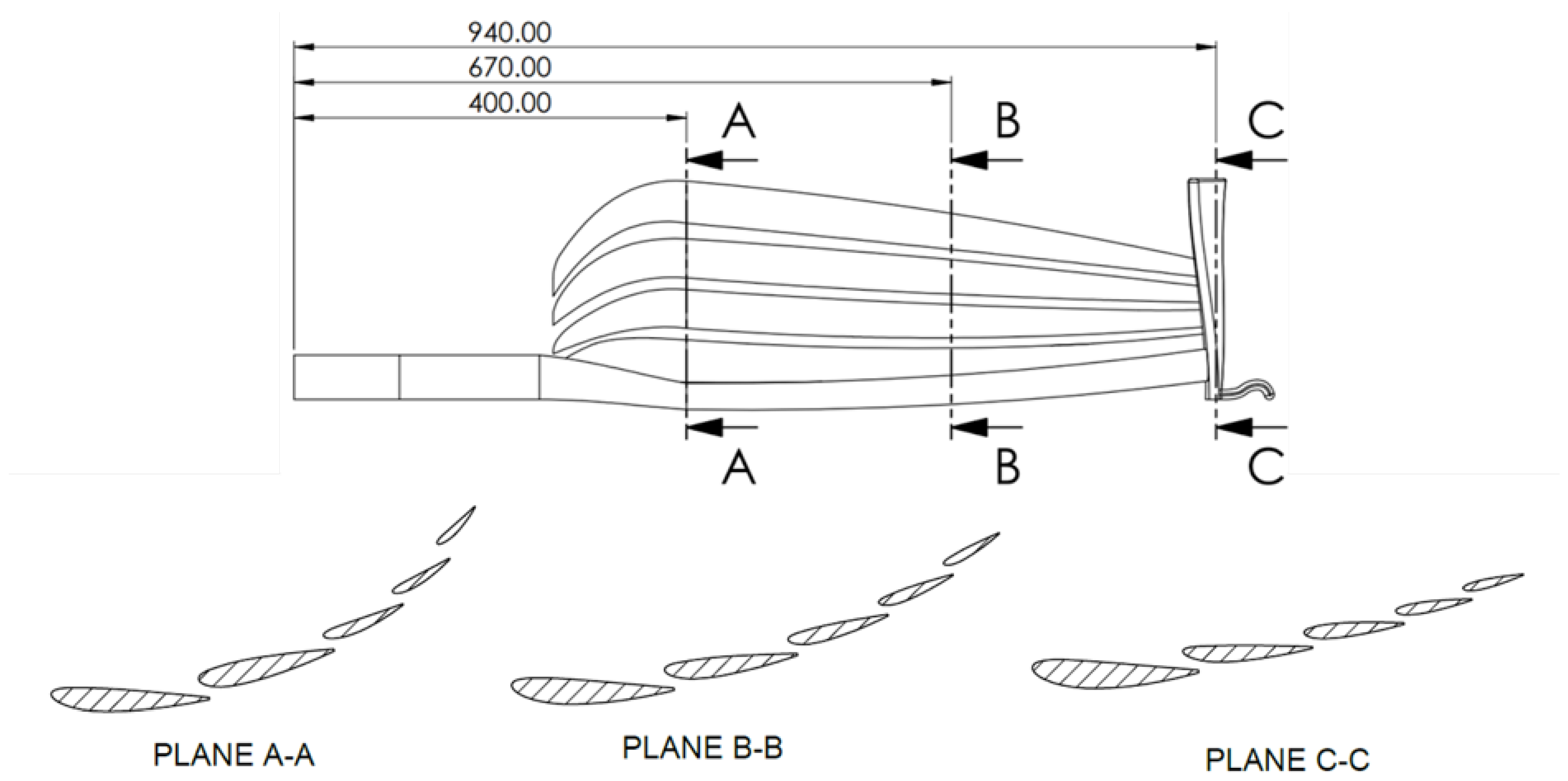
The present work is novel in both methodology and application. It aims to optimise the shape of a five-element F1 car front wing to increase downforce and decrease drag force under the FIA 2021 regulations. A five-element wing is of high complexity (computationally demanding, a high number of design parameters, airfoil–wake interactions, ground effect, different NACA profiles for each element, different NACA profiles at each longitudinal position for an element, etc.), and its optimisation has never been addressed before in the literature despite the strong interest in race aerodynamics (although it is believed that competition teams have performed optimisation studies). The only known multi-element wing optimisation has been found in [13], which considered a 2D adjoint problem and only two airfoils with a constant airfoil shape. The present investigation goes one step beyond: five elements are optimised at the same time, optimised at different positions along each element (thus, the same element’s NACA shape will vary depending on position; see Figure 1). It is also worth pointing out that, in order to create a full 3D surface from 2D studies, a series of cross-sections must be specified. It is necessary to specify at least two five-element cross-sections to be connected to form the 3D front wing; however, this would generate a linear shape. In order to create a more realistic curved shape, three five-element cross-sections (namely A-A, B-B and C-C throughout this paper) are specified, which can be connected to a three-dimensional CAD software. The FIA 2021 regulations do not permit notable changes in the curvature of spoilers (see regulations in Appendix A), so to study more than three cross-sections would not provide relevant improvements.
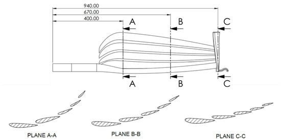
Figure 1.
View and location of the three different planes where the cross-sections for the front wing shape design optimisation have been defined.
A hybrid approach methodology is followed to achieve the best optimal five-element front wing candidate through local optimisation at three different five-element cross-sections. The proposed hybrid optimisation is a two-step approach: first, an optimal candidate (namely parametric optimisation throughout this manuscript) is obtained based on 17 design parameters, in which, to overcome the complex geometric constraints, specific restrictions are imposed. The regulations are described in Appendix A, where the limitations in the design are also discussed. Second, adjoint-based RBF optimisation will be applied to further improve the optimal candidate solution. This novel hybrid approach is more robust than direct adjoint-based optimisation since a good initial guess (the optimal from parametric optimisation) is provided to the adjoint-driven approach, avoiding local minima/maxima [55,56] or slow convergence of the adjoint approach [57].
To end up this introductory section, this paper is structured as follows: In Section 2, the methodology followed in the hybrid (parametric and adjoint) optimisation method is explained. In Section 3, details on the mathematical foundations behind the methods are given. Later, in Section 4, the CFD simulations are described, from their set-up to their validation. In Section 5 and Section 6, the results from the parametric and hybrid optimisation are discussed, respectively. Finally, the conclusions from this work are drawn in Section 7. The FIA regulations that constrained the optimal search are described in Appendix A.
2. Methodology
Due to the complexity of the simulation of a multi-element front wing and the large number of design parameters, the direct application of adjoint-based optimisation under the FIA-specified constraints is nearly impractical. For this reason, the optimisation study will be developed in two steps as a hybrid optimisation approach. The first step will consist of a parametric optimisation study using GP as the RSM approach, and the second step is the adjoint-based optimisation with MM-RBF (see Figure 2).
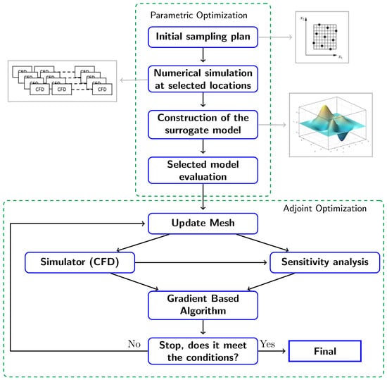
Figure 2.
Schematic overview of the optimisation framework.
2.1. Parametric Optimisation
The first step (parametric optimisation) is divided into several stages: Design of Experiment (DoE), the automatic generation of geometry, mesh and simulation, and in turn, the exploration of the response surface by means of the optimisation algorithm. The DoE determines the exact simulations (CFD sample individuals) to be run to build the response surface. The selection of individuals depends on the number of design parameters, which in this study corresponds to a total of 17 design parameters, summarised in Table 1. These parameters correspond to the parametric characterisation of profiles (NACA digits), angles of attack and position (spacing and overlap). It is worth mentioning that inside each profile a naming convention is defined to identify each NACA four-digit wing variable: chord (c), maximum camber (m), maximum camber location (p), maximum thickness as a fraction of the chord (t), and preceding it the profile (P) is identified. The input parameters vary in a continuous manner within a specific range of analysis. The range is defined by the upper and lower bounds of the parameter and then an Optimal Space-Filling Design (OSF) creates optimal space filling DoE plans according to the specified number of simulations. In essence, OSF is a Latin Hypercube Sampling Design (LHS). The objective is to achieve the most uniform spatial distribution of points (maximizing the distance between points). It must be outlined that, in order to reduce the design parameter space up to the said 17 parameters, as the fourth and fifth elements of the front wing have the smallest dimensions, these share the same NACA profile obtained for the third element but with rescaled dimensions. The scaling to be applied is a factor scale from P3_c over P2_c (that is to say, the ratio between the third and second profile chords) resulting from multiplying the fourth and fifth chord values by 0.8 successively (20% of variation). The angles were modified similarly, but with a 1.2 increase (growth of a 20%). All the constraints set by the FIA applicable to the design of the front wing are described in Appendix A. It is important to let the reader know that these constraints require certain configurations in the DoE to be discarded. That is, for instance, if the total chord of the front wing as a result of the combination of certain overlapping, angles, etc., surpasses the size limit set by the FIA, this individual from the DoE must be discarded. Thus, a corrective function is applied to rescale the profiles, recalculate their NACA, and test if they now satisfy the constraints.

Table 1.
Ranges of each variable in the parametric study.
Once a sufficient number of simulations are run (in the present work, a total of 150 simulations in the DoE was a decent number to obtain surrogate models), GP models can be built. GP are used to interpolate data and construct the response surfaces. This reduced order approximation aims at modelling the drag and lift coefficients and , respectively, as a function of the design parameters. The NSGA-II optimisation algorithm can be then used to sample response surfaces to find the optimal candidate that maximises and minimises .
It is obvious that this problem is three-dimensional. However, to deploy the optimisation framework for 17 design parameters in 3D CFD simulations would be too demanding (and nearly impractical). To overcome these restrictions, the parametric (and adjoint-based) optimisation procedure has been developed on three different key sections—A-A, B-B and C-C, as shown in Figure 1. This allowed us to perform three independent 2D computational optimisation studies, whose optimal designs can be transformed into a final 3D front wing design.
2.2. Adjoint-Based Optimisation
By using the parametric optimisation outcome as the initial (baseline) design, the adjoint-based optimisation method is applied to continue the process (Figure 2). Based on the parametric baseline mesh, the RBFmorph add-on in ANSYS Fluent (adjoint tool) is used [58]. This allows us to compute local sensitivity estimates to guide the optimisation process, by deforming the computational mesh accordingly. These adjoint-based model iterations were fixed to 20 iterations in order to achieve sufficient improvement and avoiding to keep changing shape without substantial improvement whilst diverging excessively from the baseline shape. An additional mathematical description of the method is provided in Section 3.2. Further information on how to implement the ANSYS Adjoint Solver can be found in the handbook [59].
In order to work with a morphing mesh, it is necessary to constrain the space and define a current objective output. The objective output must be controlled to perform the shape modification. In the present application, the objective output is the ratio. The adjoint method works by searching for solutions in the design space in which for each adjoint iteration the ratio is increased (reducing drag will increase vehicle speed, whilst downforce is also intended to increase). The method also requires to implement spatial contraints. In order to ensure the proper development of the adjoint-based shape modifications, a boundary box (envelope) of 575 × 225 mm was created, which is in accordance with the FIA regulations. This box guarantees that the different geometries of the profiles will not exceed the front wing workable volume established in the regulations.
3. Mathematical Considerations
3.1. Gaussian Process Surrogate Sampling with Genetic Algorithms
Response Surface Models (RSM) are used in the initial step in the optimisation process. The objective of this method is to approximate an exact model in the parameter design space by a model function with an error . Thus, the approximation takes the form [60]:
GPs approximate the exact response by means of a regression function to capture the largest variance of the training data. Later on, a Gaussian process is added to the model, so that [60]:
where Y is the vector of training data, W represents the weighting functions, represents the coefficients of the regression function and stands for the vector of basis functions in the construction of the regression model polynomials. The model consists of obtaining an approximation to the exact model by means of weighting the existing points with weighting functions to estimate the behaviour surrounding the points.
The selection of the regression function defines different types of GPs. The most general case is to model as multivariate polynomial, as carried out in Equation (2), which is popularly known as universal kriging interpolation. A simpler model consists of using a known constant, i.e., (simple kriging), which can be also generalised to a constant unknown regression such that (ordinary kriging). More elaborated data interpolations can be also developed by means of Gradient-enhanced Gaussian processes [61,62], thanks to the use of gradient information to decrease the number of samples needed to build the surrogates. This method allows us, through interpolation, to construct the response surface under the strong influence of the correlation function in . The Gaussian process has zero mean and covariance = , where is the process variance. In addition, Mean Square Error (MSE) estimates can be obtained with this method, since the GP is able to compute its predictor variance. These error estimations allow the practitioner to increase the number of points between individuals to decrease such variance if necessary [18]. This error measure is obtained by means of [63]:
where is the vector
For further information on the method, please see [64,65].
The surface is then sampled by Genetic Algorithms (GA), where Non-dominated Sorting Genetic Algorithm-II (NSGA-II) [66] is used. This GA was developed to improve the deficiencies of the popular NSGA [22,67]. This new version of the algorithm overcomes the classical difficulties in evolutionary algorithms by decreasing the computational complexity and use of elitism, and avoiding the requirement of a sharing parameter [66]. NSGA-II consists of a fast non-dominated sorting approach, much more efficient than other evolutionary algorithms existing in the literature. This is so because in order to determine the first non-dominated solutions from a total of N population size for M objectives, a number of comparisons of order must be carried out for each solution, leading to a total of computational costs just for the first non-dominated front. This process is then repeated for the next stages, leading to computational costs of order . The fast non-dominated approach suggested in [66] leads to a total of computational costs in non-dominated sorting. This reduction in computational resources is based on two calculations for each solution s: (i) A domination count (number of solutions that dominate s) and (ii) to set a group of solutions dominated by the solution s. This process is carried out at the different front levels to rank the solutions according to the level of domination. To allow a certain level of spreading in the solutions from the method, the original NSGA used a sharing function approach. This function involves the sharing parameter (input to the algorithm) to compute distance measures between two individuals. To avoid this dependency, the NSGA-II incorporates a crowding-distance calculation, which consists of creating a cuboid whose vertices are extended up to the nearest neighbours (upper and lower limits) around a particular solution . This allows the computation of how crowded a solution is, what supports the selection process towards more uniform Pareto fronts: the logical operation (called crowded-comparison operator) for classification is that (i) between two solutions with different ranks, the one with the lowest rank is selected; (ii) however, if both solutions share the same rank (are at the same front), then the one with the lowest crowding distance is selected. To summarise the full process in one iteration (see Equation (5) below), from a population set of N samples, genetic recombination and mutation operators are applied to create the new additional samples . These samples (the samples from the union of and ) are sorted according to non-domination, and elitism is guaranteed at this point since all initial samples are included in the population of size . The samples are now sorted according to the front rank, and from these, only a total of N samples are selected, which will be chosen according to the aforementioned crowded-comparison operator. The selected samples conform the sample. The process is then repeated until convergence. Elitism is ensured in the algorithm since the best previous optimal samples are included in the following population sets: This supports the convergence of the method, as optimal candidates already found are not lost during the next iterations. For further details on the method, see the original paper by Deb et al. [66].
3.2. Adjoint Approach to Optimisation
CFD-based shape modification can be developed through mesh geometry modification via MM-RBF, instead of developing a new geometry via CAD and its mesh every time. This more efficient approach includes both the interior as well as the boundary nodes. In this case, mesh geometry is created upon control variables, since in engineering problems the mesh geometry can be modified for a more optimal performance according to the iterative evaluation of the objective function. Thus, the adjoint solver is coupled with the flow solver. This coupling allows the quantification the influence of variations of design variables on the performance. The goal of the adjoint method is then to determine the sensitivity of the objective function with respect to the user-specified control variables. The linearisation of the objective function can be represented by the equation
with q being the flow state variables and c the control design variable. Thence, the derivative of the objective function depends on the flow state and the control variable, which can be expressed as
where denotes variations of flow state variables and denotes variations of control variables [68]. The derivative of the objective function is therefore the superposition of two partial derivatives: one for the geometric sensitivities and another for the flow field sensitivities. The very important advantage of the use of the adjoint method is that the flow state-dependent part can be rewritten as dependent on control parameters.
With the governing Navier–Stokes equations written as
then
This equation basically means that when the flow field changes, is zero. To transform the nature of the optimisation problem from a constrained into an unconstrained problem, the Lagrange multiplier can be used by combining and . Thus, can be written as
By grouping the terms multiplied by and , respectively, the vector of adjoint variables can be chosen so that there is no influence of flow variables in the computation, which leads to the adjoint equation to be solved [69]:
3.3. Radial Basis Functions
In this work, adjoint-driven shape modifications in the CFD domain are developed according to a mesh morphing technique. This technique consists of the use of Radial Basis Functions (RBF). This method evaluates the distance between points by means of the Euclidean norm as
where is the radial function, which can be either linear, multiquadratic, cubic, Gaussian or thin flat spline [29]; b is a constant with , and is a polynomial approximation function. This polynomial fit of order n can be expressed as
where are the polynomial coefficients and are the basis of polynomial functions for the span. To obtain the coefficients from Equation (14) and the coefficients from Equation (13), the RBF approximation must satisfy that the provided values at the known source points coincide with the RBF value at these points [32]:
and the orthogonality condition:
with the number of samples. In RBF mesh morphing, the sampling points are interpolated in space for the mesh nodes to be adapted to their new position (morphing). Together with the adjoint sensitivity calculation, the mesh is then adapted to a new shape driven by the calculated sensitivities. Further details on RBF (including different radial functions and its fast version) can be found in [31,32].
3.4. Governing Equations Turbulence Modelling
The governing equations in fluid mechanics are the Navier–Stokes equations, which are solved numerically by the software ANSYS Fluent. The Reynolds-averaged Navier–Stokes (RANS) continuity and momentum equations can be written in cartesian tensor form as [70]:
where represents the velocity components, shows the velocity fluctuation components, represents spacial coordinates, and overbars represent averaged quantities. The term stands for the Reynolds stresses, which is modelled according to the selected turbulence model closure. In this work, the Boussinesq hypothesis is applied, selecting the eddy viscosity turbulence models such as the Shear Stress Transport (SST) turbulence model. The SST model was developed by Menter [71]. It assimilates the boundary layer between the eddy viscosity and full turbulent viscosity formation. The SST model draws up the best effects of (accurate at far-field region) and (good accuracy at near-wall region). The is modelled as
where k is the turbulence kinetic energy, is the dissipation rate, is the turbulent viscosity, () refers to the generation of turbulence kinetic energy as a consequence of velocity gradients (buoyancy), stands for the fluctuating dilatation in compressible turbulence to dissipation rate, , , and are empirical model constants, and are the turbulent Prandtl number for k and , and and are user-defined source terms for each equation. The turbulence model also prevents being too sensitive to the inlet free stream turbulence. For this model, the two additional closure equations in compact notation for k (turbulent kinetic energy) and (specific turbulent dissipation rate) are:
where and are the effective diffusivity of k and , and are the generation of k and due to mean velocity gradients, and and are the dissipation of k and , respectively. is the cross-diffusion term. For further details, please see [72].
4. CFD Simulation
The CFD simulations carried out in this optimisation work consisted of three 2D cross-sections of the front wing, which consists of a total of five airfoil elements per simulation. This simulation is quite complex, as there is an interaction between several front-wing airfoils, which will be also further deformed by the MM-RBF approach. Thus, these simulations have been first validated and tested, in order to use a suitable mesh. At the end of the day, this 2D approach allows us to recreate the final full 3D front wing by connecting the three optimal 2D cross-section sections of the front wing e.g., via CAD software.
4.1. Set-Up of the CFD Simulations
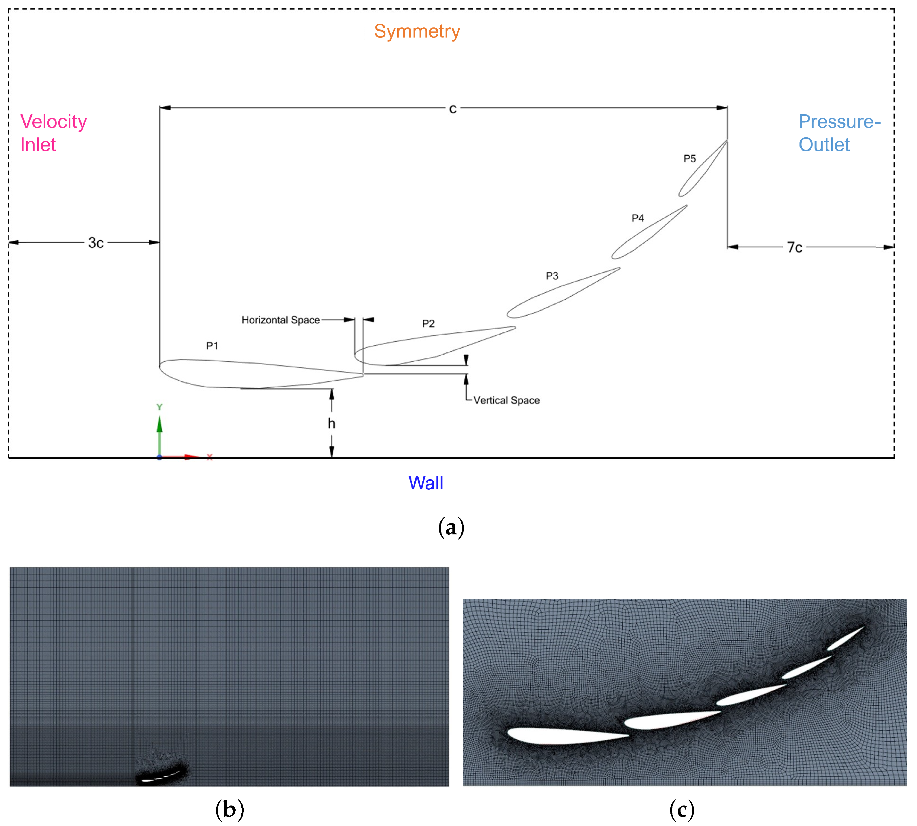
All CFD simulations have been run in ANSYS Fluent. The solver has been configured on a pressure-based formulation with air as working fluid. The numerical scheme corresponds to a second-order spatial discretisation, and the Semi-Implicit Method for Pressure-Linked Equations algorithm to solve the pressure-velocity coupling. Boundary conditions are imposed on the simulation to solve the Navier-Stokes equations. The boundary conditions imposed are shown in Figure 3 and correspond to Wall boundary condition on the airfoils and ground; Velocity-inlet at the inflow of the domain; Pressure-outlet at the outflow of the domain; and Symmetry at the top of the domain. More specifically, the Velocity-inlet is a uniform velocity profile of m/s. The selection of an inlet velocity of 30 m/s is founded on the aspect that wind tunnel testing of entire racing cars is carried out on reduced size models lower or equal to 50–60% of the real car size, and at wind tunnel speeds not exceeding 40 m/s [73,74]. This means that the Reynolds number is sufficiently high. In our simulated five-element front wings, the Reynolds number was of order (with the mentioned velocity, air as working fluid, and a total five-element chord of approximately mm). On the other hand, the performance of the ailerons can be also estimated from slow/medium velocity curves. On the very popular Autosport resource [75], it is explicitly said that “Hungary, Imola, Singapore, Spain and Monaco are all examples of high downforce tracks, with relatively short straights and lots of turns putting a greater emphasis on cornering speed". Actually, as outlined in the article, the performance in one of these tracks can be used to estimate the performance in others due to the series of low-speed turns. It is likely that selecting lower speeds in the simulation could give us a design not suitable for all types of circuit. Thus, with our decision, we could relate our designs with existing wind tunnel data and, moreover, the selected velocity is quite consistent with increase in downforce and reduction in drag in popular race tracks. Thus, for all these reasons, 30 m/s was considered a very good option as inlet velocity. The Wall boundary condition on the ground is imposed as a 2D moving plate with the same velocity, and as static for the airfoils. In both cases, the surfaces are adiabatic and non-permeable, with non-slip velocity boundary condition . The Pressure-outlet boundary condition on the outflow is imposed to satisfy the atmospheric pressure, and gradients are fixed to zero value for the transported quantities. The Symmetry boundary condition at the top is used because the upper boundary is far enough from the wings so that the inlet velocity profile is nearly invariant across it. More concretely, the upper boundary condition is located at 10 times the existing distance from the floor to the highest point of P5. at the top is just a mathematical calculation to satisfy a zero flux of all quantities across its boundary.
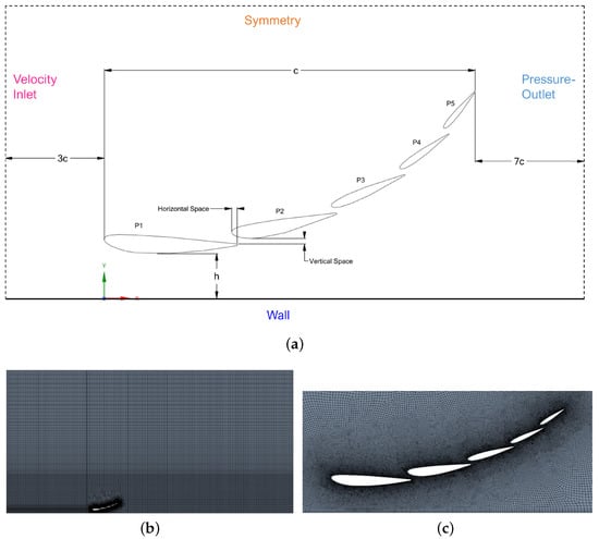
Figure 3.
Sketch of (a) computational domain including boundary conditions, (b) computational grid, and (c) detail of computational grid around the front wing.
The geometry of the front wing is created automatically according to the parametrisation of the NACA airfoils and their distribution along the domain. The parametric aerodynamic profiles were designed in ANSYS SpaceClaim using IronPython, which is an open-source language built on Python. Each profile is based on four NACA parameters, producing airfoils of any thickness, thickness distribution, or camber [76]. Complying with the restrictions imposed by the F1 regulations, the code readjusts the input variables for each profile, as well as the spaces between them, as explained in Section 2. A sketch of the boundary conditions applied to the geometry is shown in Figure 3, where a five-element cross-section of the full wing is shown. The c parameter represents the total chord of the front wing, and h is the separation from the ground. The upstream distance from the wings must be long enough for not being affected by the front wing. For this reason, a distance of has been chosen, so that the fluid can adapt consistently from the inlet to the presence of the wings. Additionally, the downstream distance from the front wing must be also large enough so that the near wing region (and its flow structures) are not affected by the imposed boundary condition at the outlet. For this reason, the downstream region has been extended up to a distance from the front wings.
4.2. Validation of Simulations
Convergence Analysis of the Full Front Wing Mesh
The CFD simulations have been carried out as 2D planar simulations using the SST turbulence model, at uniform m/s, which was a velocity value robust in experimental test rigs in [73]. The use of this turbulence model in turbulent simulations of airfoil applications has been vastly studied in the literature demonstrating that it is a suitable model for this application and providing a very good match with experimental data [77,78,79,80]. As additional information, current wind tunnel testing of entire race cars is performed using models not greater than 50% scale, at speeds lower than 40 m/s. Actually, in the present study, the reference speed and model size correspond to Reynolds numbers in the range of approximately 20% to 50% greater than current race car model testing. The under-relaxation factors used for pressure, density, force, momentum, and kinetic energy, have been 0.3, 1, 1, 0.7 and 0.8, respectively.
The grid convergence study was performed by developing three different meshes: with a coarse, medium, and fine grid of a straight airfoil blade with ground effect (with height ) to determine how the mesh quality affects the CFD simulation results. The Reynolds number according to this 1-element wing chord of mm is . Both the number of nodes and the elapsed time for the three cases simulated using the SST model are highlighted in Table 2. The meshes generated have near-wall resolution with a . There is very little difference between the medium and fine mesh, as well as with the experimental value, so the medium mesh will be the one replicated in the five-element front wing. The convergence of simulations was found after approximately 100 iterations, as observed in all residuals below . To be conservative, once all residuals were below , the simulations were run up to a total of 200 iterations.

Table 2.
Mesh size, elapsed time, and calculated values of for validation and convergence analysis on a single airfoil.
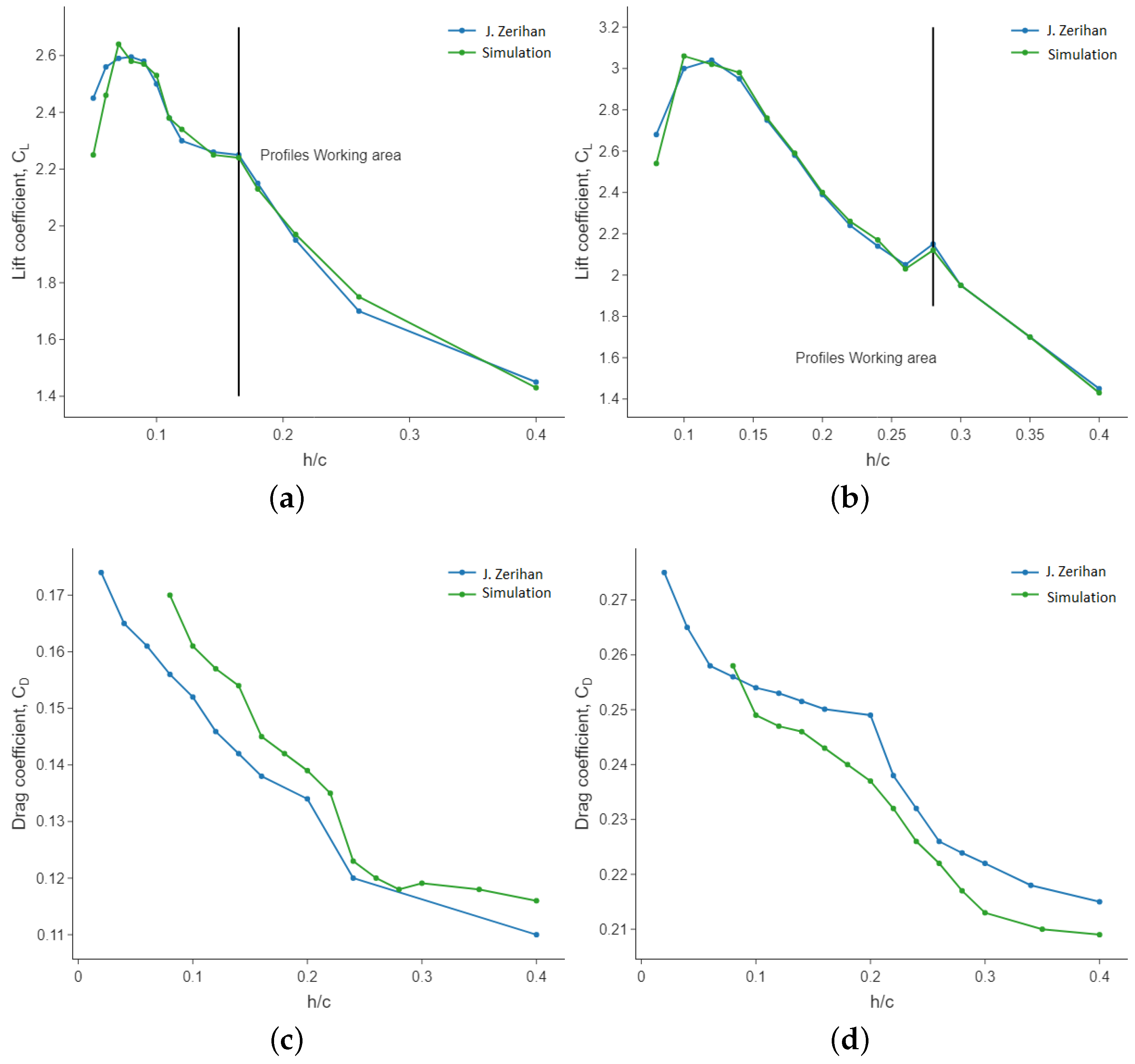
Finally, as the front wing consists of several elements in cascade, the interaction between profiles and ground effect has been tested by means of a mesh of similar characteristics to the medium mesh achieved in the convergence analysis. To validate the simulations, CFD simulations of a 2-element wing with ground effect at a similar Reynolds number of the race car experimental performance test in [73] are developed. The Reynolds number according to this 2-element wing chord of mm is . In Figure 4, the performance of the downforce (lift coefficient) and drag force (drag coefficient) of a 2-element front wing is tested at different heights ( ratio) and compared to the experimental data reported in [73]. In their work, the first element is always fixed, and the second profile has two possible deflection angles (low and high flap angles, of −8.5 and +9.5 degrees, respectively). The match between the experimental data and the present simulation shows that the computational simulation is quite accurate and the search for an optimal candidate via CFD is reliable.
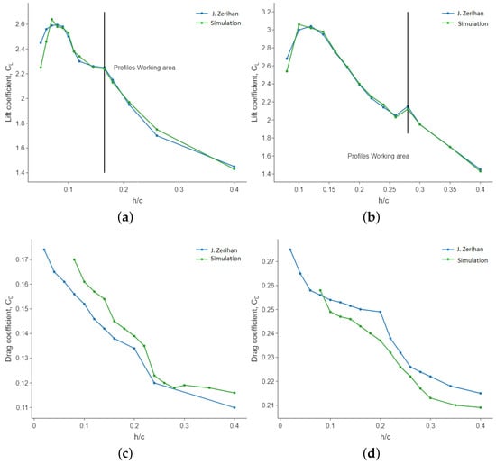
Figure 4.
Results of 2-element cascade front wing simulation with ground effect at different heights for downforce with (a) Low flap angle, and with (b) High flap angle; as well as for drag with (c) Low flap angle, and with (d) High flap angle. Reference data from J. Zerihan [73].
5. Results from Parametric Optimisation
The design space introduced in Table 1 is explored by the optimisation algorithm on the GP surrogates to obtain the final optimal parametric front wing. This optimal design becomes the initial guess for the iterative adjoint-based approach in order to perform a hybrid optimisation.
5.1. Exploratory Analysis
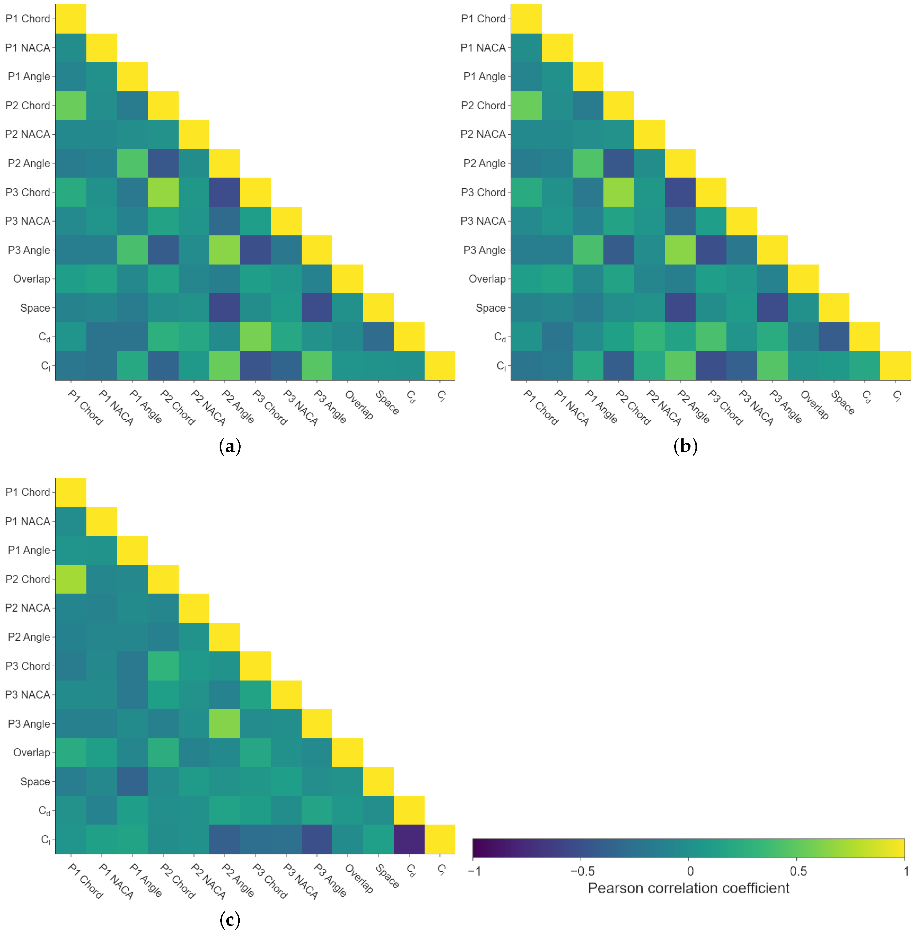
An initial exploratory analysis was carried out to evaluate the surrogates with a 172 random samples (at least 4 sampled points per design space variable) in order to determine whether any relation between variables is strong enough to reduce the number of design variables or redo the value ranges shown in Table 1. The computational time was approximately 0.2 CPU hours for each design. The drag and lift coefficients are also shown in order to analyse any potential remarkable relationship with the inputs. In Figure 5 it is shown the Pearson correlation between variables for the three cross-sectional planes. It must be recalled that some variables from Table 1 are strongly related to other variables. More concretely, parameters related to Profile 4 and 5 are not shown, as there is a geometrical relation with other design space parameters imposed beforehand. This was done to limit the design space and reduce the number of samples. Thus, Profile 4 and 5 have the same NACA profile as Profile 3: their respective angles are shared with Profile 3 with an increase of a 20%, just like with the changes in chord, in which the code included a reduction of a 20%. The only relations worthy of discussion in Figure 5 are observed for the chords, which is something predictable as the FIA regulation constraints related to the maximum and minimum sizes of the front wing are applied. Thus, a chord influences the other as its chord is adapted to the existing space. In other words, due to the FIA regulations, there is a limit in the maximum length of the front wing geometry. Therefore, a change in the chord of a profile restricts the chord size of the rest, as well as the separation between profiles, in order not to violate the regulations. The angles also exhibit some degree of correlation, especially in A-A and B-B cross-sections. However, these are reasonable. A zero-value correlation would mean that variations in the angle of an airfoil do not influence others, which is not realistic. Thus, the relations between parameters seem consistent.

Figure 5.
Parameter exploration via Pearson correlation for (a) A-A cross-section (400 mm), (b) B-B cross-section (670 mm), and (c) C-C cross-section (940 mm), of the five-element front wings from the specified input design variable ranges.
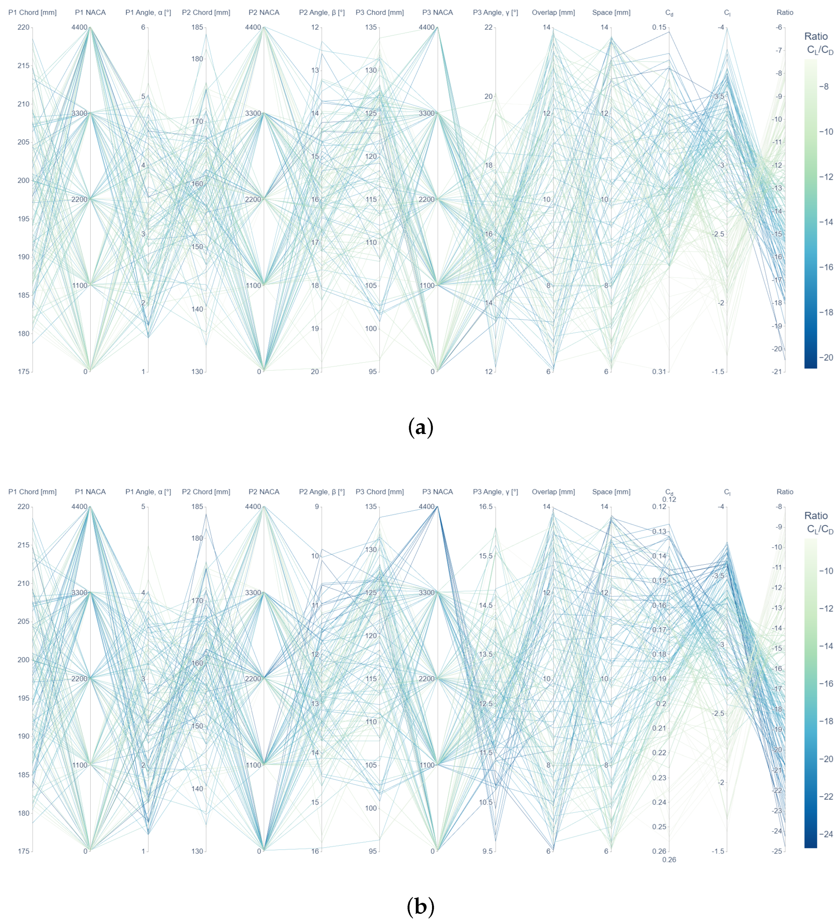
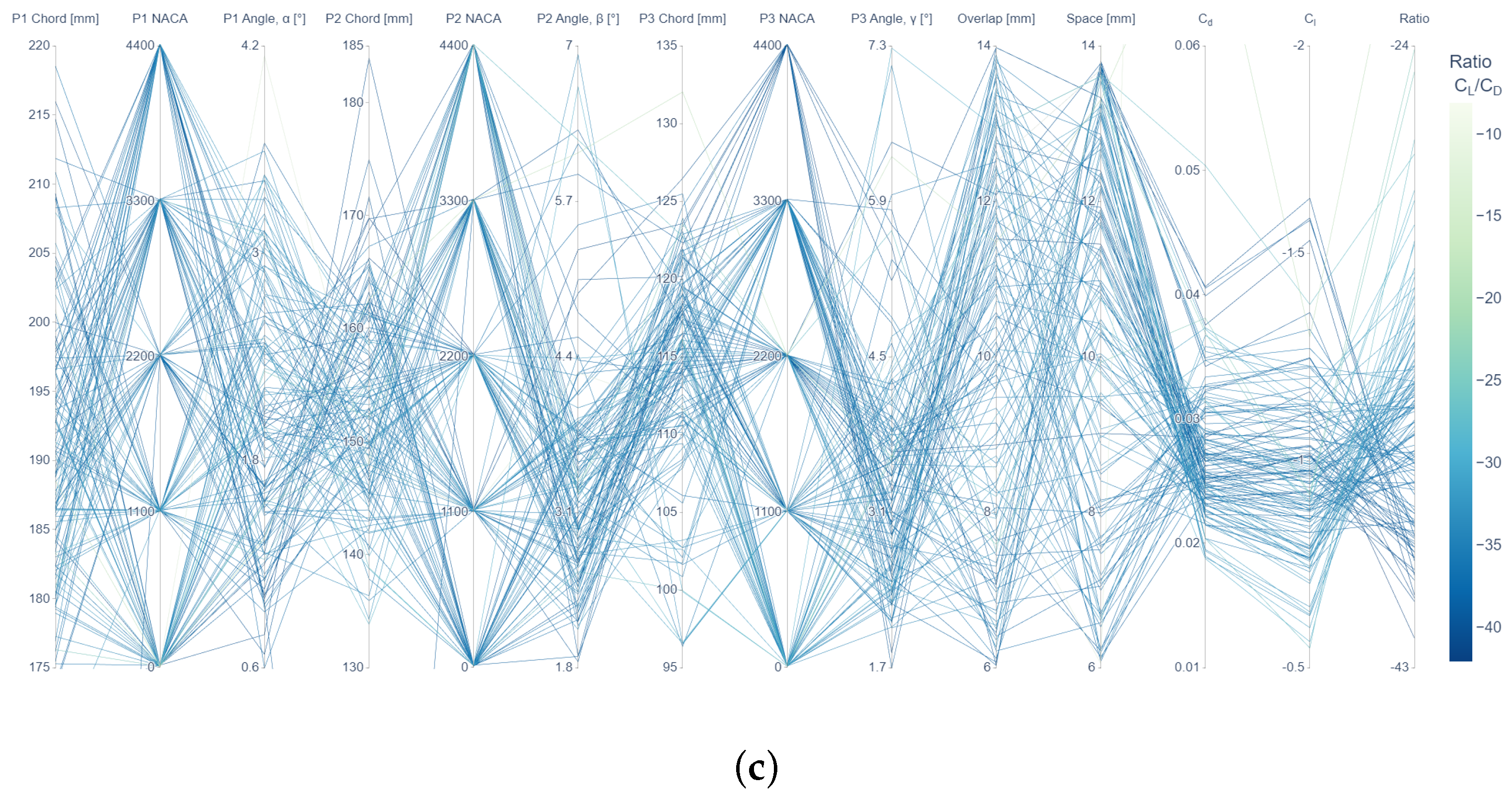
Parallel Coordinate Plots were also used to explore the relations between parameters. This type of plot allows us to observe the best paths to achieve the expected optimal design (increased downforce over decreased drag). As observed in Figure 6, it is very complex to determine a specific value or narrow range for each parameter to obtain the optimal design(s). These plots show that the problem mechanics have a strong underlying non-linear relationship. From the three planes shown in the figure, it is observed more convergence to desirable solutions in the C-C cross-section (Figure 6c), as most sampled designs yield a low ratio, reflected by the dark colour in the colour range. Also, for these designs, the ratio is the lowest. On the other hand, the A-A cross-sectional area (Figure 6a) exhibits less promising outcomes, because there is a range of potential solutions that could result in a relatively good design, but a clear path (selection of design parameter values) cannot be identified. In other words, the connection between good candidates is more diffuse in this cross-sectional area.
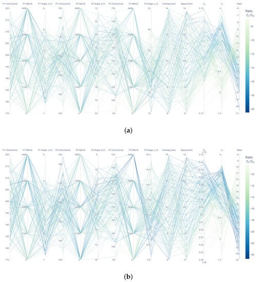
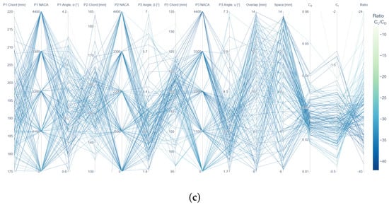
Figure 6.
Parameter exploration via Parallel Coordinate Plot for (a) https://plotly.com/pablomh/16/, A-A cross-section (400 mm), (b) https://plotly.com/pablomh/18/, B-B cross-section (670 mm), and (c) https://plotly.com/pablomh/20/, C-C cross-section (940 mm), of the five-element front wings from the specified input design variable ranges. Please note that hyperlinks to Plotly graphs are included in the electronic version of this paper for interactive visualisation of the results.
5.2. Optimal Parametric Design
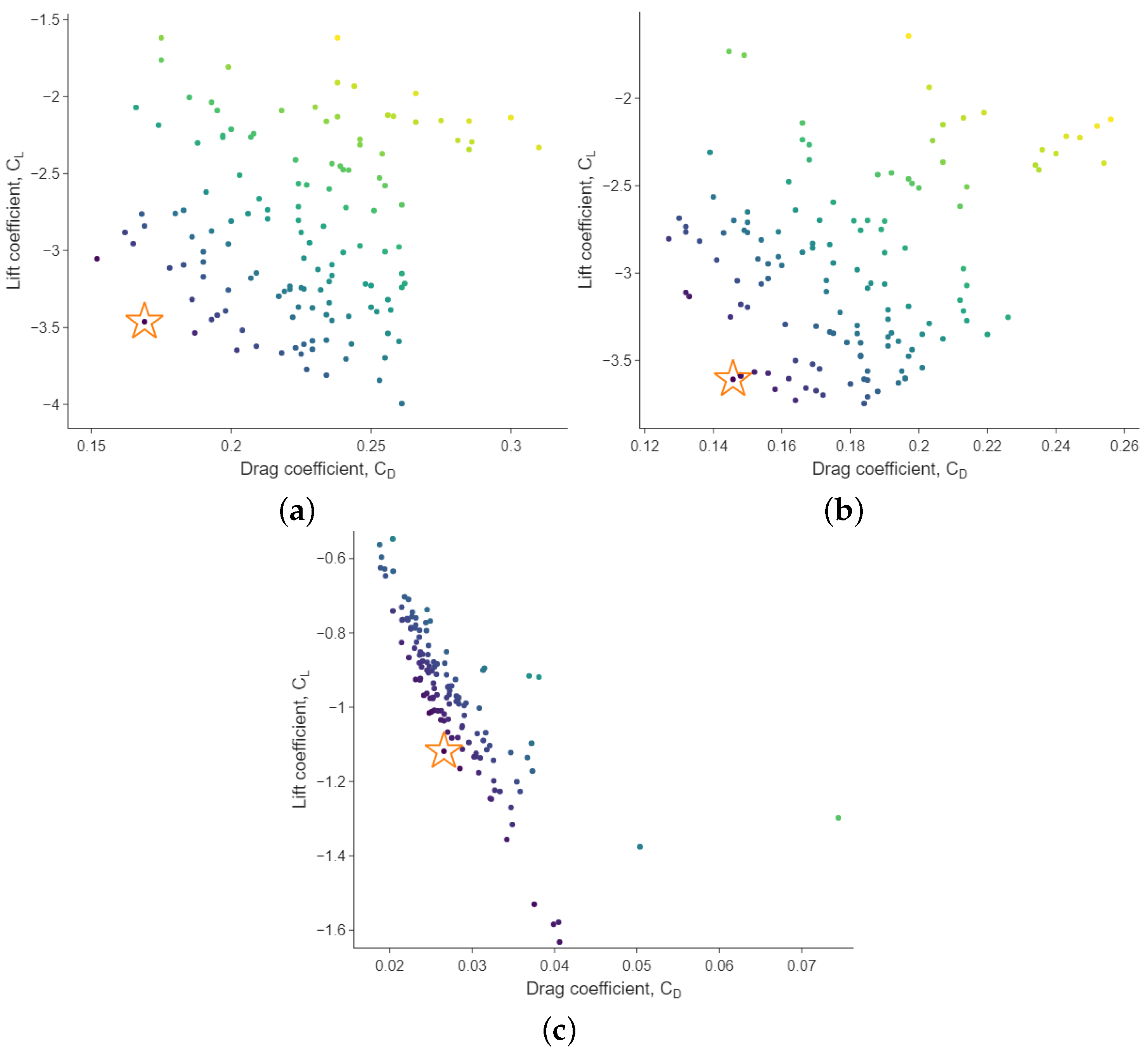
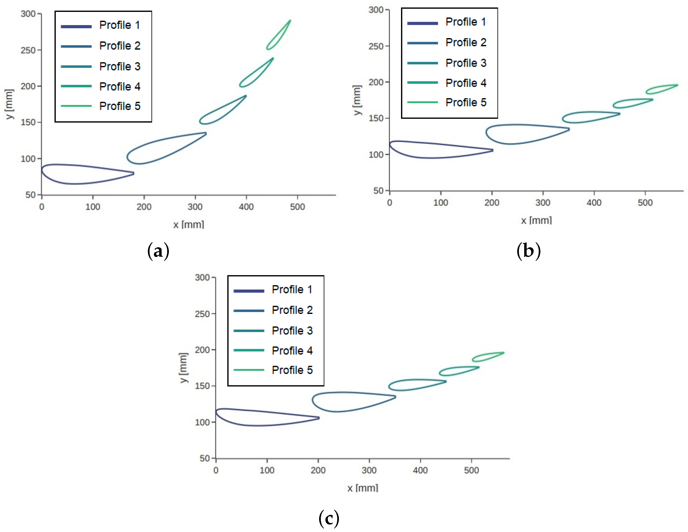
From the application of the NSGA-II optimisation algorithm on the Gaussian Process surrogates, an optimal parametric solution is obtained quickly. Although the maximisation of the ratio between and could be a single objective, it is a better practice in this type of aerodynamic performance optimisation problems to deal with and separately. This is beneficial because it is possible to find a better balance between the optimal solutions and the final desired performance, since one may need, for instance, a stronger downforce by increasing slightly the drag. This complicates the optimisation problem as it is transformed into a multi-objective rather than a single-objective, leading to a set of dominated and non-dominated solutions. The non-dominated solutions for each cross-sectional plane can be identified in Figure 7, from which a design is selected as optimal for each cross-sectional front wing highlighted with a star symbol. The optimal solution is selected amongst the configurations as the one with the lowest ratio, meaning the lowest drag with the highest negative lift (downforce) in each plane. To ensure enough degree of confidence in the selection of an optimal candidate, a near neighbour criteria has been applied: at least other two neighbouring candidates should lie inside the of variance for both the drag and lift coefficients. The colours of points in Figure 7 stand for how far designs are from the selected optimal candidate (the closer, the darker). The front wing designs are shown in Figure 8. The parametric configuration of these designs is given in Table 3. These selected designs provided the following performances: for the A-A plane, for the B-B plane, and for the C-C plane. These designs will be the baseline design for the adjoint-based optimisation solver in ANSYS Fluent.
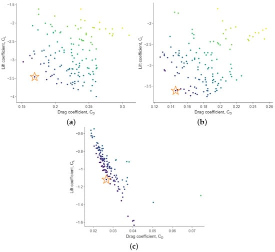
Figure 7.
Dominated and non-dominated optimal parametric designs for the (a) A-A cross-section (400 mm), (b) B-B cross-section (670 mm), and (c) C-C cross-section (940 mm), of the five-element front wings from the specified input design variable ranges.
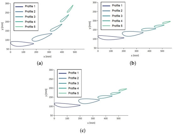
Figure 8.
Optimal parametric designs for (a) A-A cross-section (400 mm), (b) B-B cross-section (670 mm), and (c) C-C cross-section (940 mm).

Table 3.
Optimal front wing profiles from parametric optimisation.
6. Results from Hybrid Optimisation: Final Design
Once the parametric optimal design is available, one can explore further improvements on this front wing design via the MM-RBF adjoint-based optimisation add-on in ANSYS Fluent, performing so a hybrid optimisation approach.
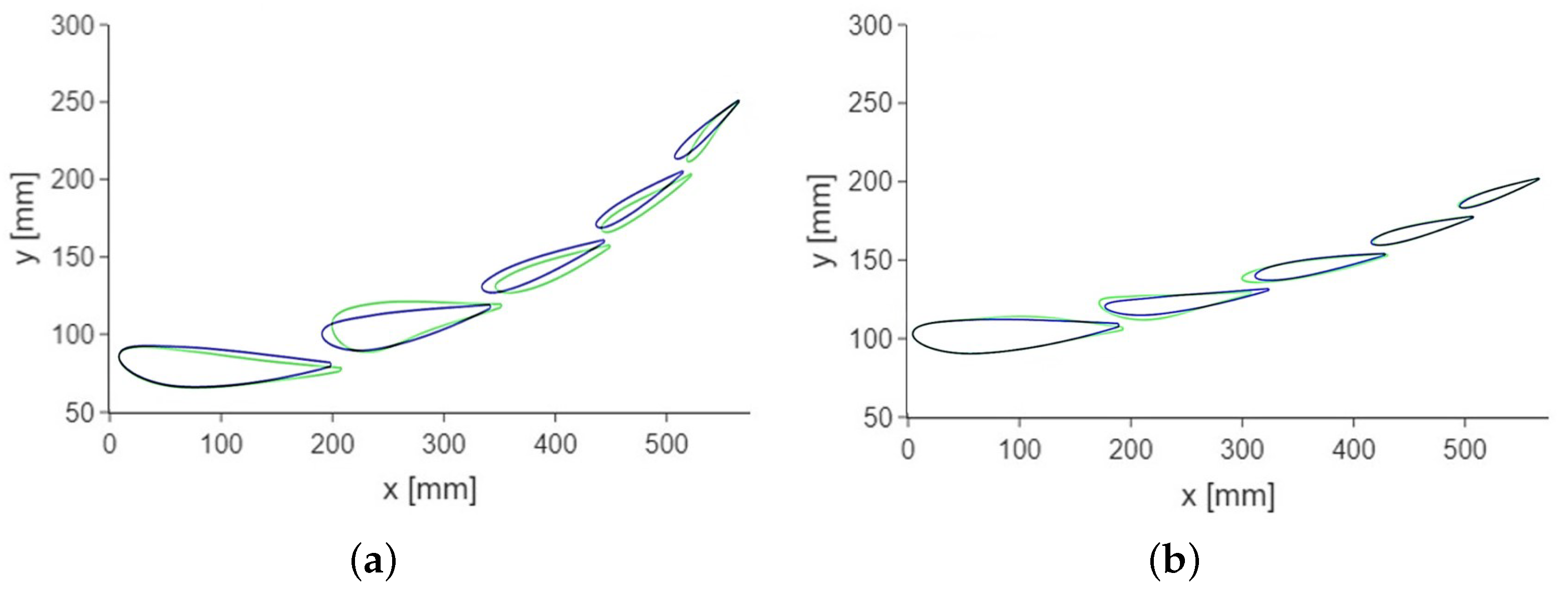
Due to the high degree of freedom in adjoint calculations, the adjoint-based optimisation strategy was carried out carefully. First, in order to avoid uncontrolled divergence in results, the A-A plane cross-sectional airfoils are fixed to their parametric optimum solution. That is to say, only the B-B and C-C plane cross-sectional airfoils are optimised via the adjoint approach. As a side effect, this also allows fair comparison with parametric optimisation results. Second, at this point, the problem is treated as single-objective, aiming at maximising the ratio. The morphing limits in the MM-RBF adjoint approach are set according to the FIA regulation in [81]. This geometric constraint has been applied to the five elements (airfoils) that conform the front wing. Finally, after some preliminary testing, it was observed that a total of 20 iterations was enough to achieve optimal solutions with no remarkable improvement from 20 iterations on. The results when increasing the number of iterations are shown in Table 4. The initial guess (number of iterations equals zero) corresponds to the parametric optimal front wing, which, compared to the results at the 20th adjoint iteration, reveals the important improvement achieved with the hybrid optimisation approach. A visual comparison by superposition between parametric optimal and hybrid optimal front wings can be also seen in Figure 9, where it is noticed an important change in the shape and distribution of the five elements of the front wing. The new front wing obtained by hybrid optimisation has been able to considerably decrease the drag in the B-B plane cross-section while also increasing the downforce. For the C-C plane, surprisingly, although the drag was slightly increased, the downforce was increased very notably, being the ratio considerably improved.

Table 4.
Adjoint optimisation results up to 20 iterations.
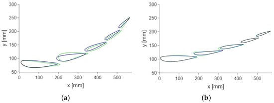
Figure 9.
Visual differences between parametric (color blue) and hybrid optimal designs (color green). (a) Plane B-B, and (b) Plane C-C.
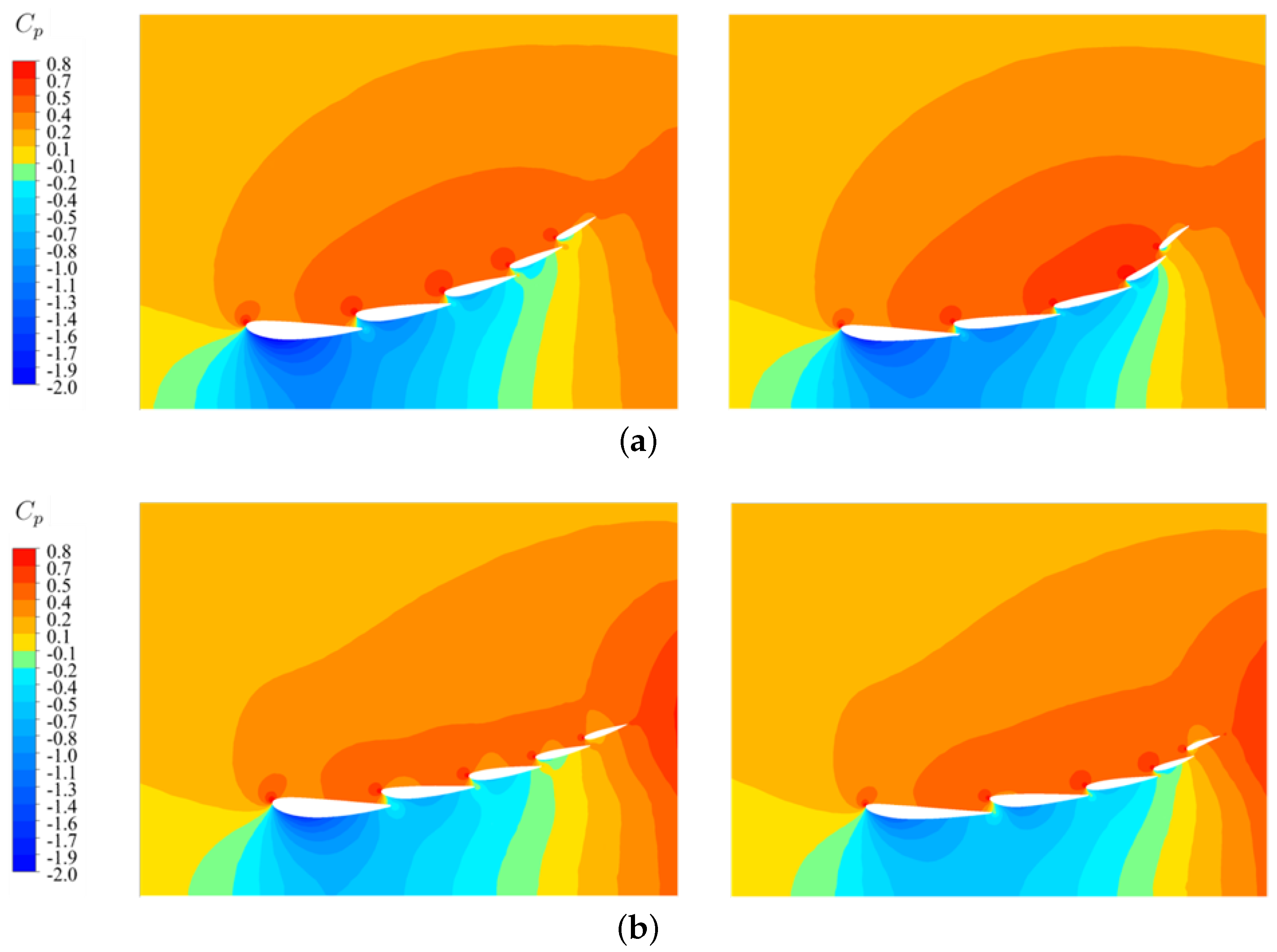
To gain more knowledge about the differences in the performance of the front wings, the pressure coefficient has been also compared between the parametric and hybrid optimisation profiles, as illustrated in Figure 10, where just a detail of the domain around the wings is shown. Figure 10a shows important improvements in the B-B plane: it can be observed that the negative values of pressure (suction effect, blue colors in the colorbar) are distributed up to Profile 4. On the upper side, pressure is higher in the hybrid optimal front wing, especially on the last three profiles. Similarly, in Figure 10b the comparison between the parametric and hybrid optimal profiles shows improvement. At the bottom side, although the first profile exhibits less suction, the rest of the profiles have a clear increase in suction, which, together with the pressure increase at the upper side of the profiles, increases downforce. To end up the optimisation process, a final shape of the actual 3D front wing design can be obtained by using a CAD software that interpolates with splines the three 2D optimal five elements to define the 3D design. The proposed 3D design is shown in Figure 11.

Figure 10.
comparison between parametric (left) and hybrid (right) optimal front wings for (a) B-B cross-section (670 mm), and (b) C-C cross-section (940 mm).
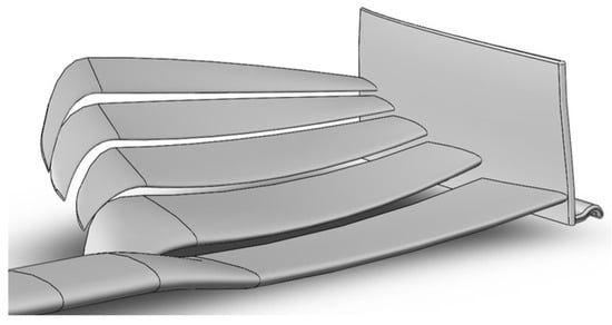
Figure 11.
Final proposed 3D design by the hybrid optimisation approach.
Therefore, the application of the MM-RBF adjoint-based optimisation has led to an improvement of the ratio of coefficients of up to 25% for the B-B plane and 14% for the C-C plane (see Table 4). This important enhancement, together with the previous search of the parametric optimal candidate, shows that the hybrid optimisation via a 2D approach is a useful and efficient procedure to design an F1 race car front wing under the FIA regulations.
7. Conclusions
In this paper, we have investigated the application of a computationally efficient 2D-based hybrid optimisation approach (parametric optimisation plus adjoint-based optimisation) for the design of an F1 race car five-element front wing constrained by the FIA regulations, for which there are no studies in the literature. The process started with the search for an optimal parametric design of the front wing from a Space-Filling Design of Experiment to construct Gaussian process surrogates. These are later sampled by a NSGA-II algorithm to obtain a set of solutions. A specific solution is then selected to later use the Mesh Morphing Radial Basis Function (MM-RBF) adjoint optimisation with the CFD code. The 2D-based approach is less computationally intensive than a 3D computational simulation problem, and by selecting strategically different cross-sections along the front wing, the procedure allowed to obtain a final 3D front wing quite fast in comparison to a full 3D simulation environment of such a complex five-element front wing realistic design under a large design space of 17 design parameters.
From this approach, the application of adjoint optimisation under the FIA regulation constraints led to the selection of a potential optimal five-element front wing that exhibits a local improvement of up to 25% with respect to the parametric optimal one. Pressure coefficient contours have also shown that the improvements in the geometric design increase the suction effect at the bottom side of the front wing, and increase the pressure force at the upper side, whereas the drag coefficient is decreased at the same time (except for the C-C plane cross-section, where a slight increase in drag is observed, but the lift-to-drag ratio is highly improved). Hybrid adjoint-based optimisation exhibits two relevant aspects that makes this a very attractive optimisation approach to refine the parametric baseline.
First, by considering that the time per case is approximately 0.64 CPU hours (thanks to the use of a converged solution as initialisation) and with a search space of 172 points (CFD simulations), an optimal parametric solution is achieved after 110.08 CPU hours. After the selection of this optimal solution as the baseline, the adjoint simulation only increases the total CPU computation by 1 hour, yielding an enhancement in design performance of around 10–20%. This improvement at the last computational stage is an important advantage compared to a full search in the entire parametric space (17 parameters), and there is no guarantee to find such a degree of improvement in any parametric search. The reason behind this actually connects with the second aspect to outline from our adjoint-based approach.
Second, the profile shapes obtained from the adjoint approach do not belong to a library or standardised classification of aerodynamic profiles, and thus solutions are strictly adapted to the problem conditions. The adjoint alone may not be able to generate profiles that meet all the requirements imposed, but by starting from a good parametric baseline candidate and by controlling its evolution an outstanding final candidate can be obtained in a relatively short time.
Although the performance of the 3D front wing obtained from this 2D approach would be more optimal than a non-optimised front wing, a full 3D simulation environment would be actually a more accurate approach (but undoubtedly more computationally costly) as 3D effects/interactions would be considered. However, it must be the decision of the engineers whether the computational costs of the process are affordable or not. If the computational budget is low and/or a new front-wing design must be obtained quickly (a common situation in F1 in order to gain advantage over competitors), then the proposed alternative is of high interest. As a latter stage, the performance of the 2D optimal adjoint-based front wing can be further tested via 3D simulation by creating the 3D shape with a CAD software by using splines. This can be simulated in CFD to extract conclusions on whether or not this final design is efficient before manufacturing it for the F1 car. This is the aim of starting with a 2D optimisation process: to finally achieve a model which can be turned into a 3D design without requiring a full 3D design optimisation environment. Another limitation of the present work is that it would be of interest to study the effect of this front wing downstream on 3D key elements of the F1 car geometry. Future work could then be related to extend this analysis with 3D simulations on the interaction of the front wing vortical structures and race car elements such as wheels and/or car frame.
Author Contributions
Conceptualization, F.-J.G.-O., P.M.-H. and J.O.-C.; Methodology, F.-J.G.-O. and P.M.-H.; Software, P.M.-H.; Formal analysis, P.M.-H.; Investigation, F.-J.G.-O. and P.M.-H.; Resources, J.O.-C.; Data curation, A.L.-M.; Writing—original draft, F.-J.G.-O.; Writing—review & editing, F.-J.G.-O., J.O.-C. and A.L.-M.; Visualization, P.M.-H.; Supervision, F.-J.G.-O., J.O.-C. and A.L.-M.; Project administration, J.O.-C. All authors have read and agreed to the published version of the manuscript.
Funding
The authors want to acknowledge the financial support from the Ramón y Cajal 2021 Excellence Research Grant action from the Spanish Ministry of Science and Innovation (FSE/AGENCIA ESTATAL DE INVESTIGACIÓN), the UMA18-FEDERJA-184 grant, and the Andalusian Research, Development and Innovation Plan (PAIDI—Junta de Andalucia) fundings.
Data Availability Statement
The datasets used and/or analysed during the current study are available from the corresponding author on reasonable request.
Acknowledgments
This research has been developed partially thanks to the Link by UMA-ATECH “K-Project” Program of the Universidad de Málaga (MART, Malaga Racing Team).
Conflicts of Interest
The authors declare no conflict of interest.
Appendix A. Formula 1 Technical Regulations 2021: Front Wings
A front wing works in the opposite way of how an aircraft wing works. The airfoil of a front wing is profiled so that it helps to attach the car to the ground, promoting the contact of wheels with the surface. Thus, the front wing plays a major role in ensuring sufficient grip for the car. In addition to the effect on the downforce, front wings also control the total airflow surrounding the car, by directing the airflow in a way that optimises the aerodynamics of the full car.
The geometrical constraints of the front wing can be observed in Figure A1. The total front wing volume is comprised by 2000 mm in width, 575 mm in length, and a minimum and a maximum height of 75 and 300 mm, respectively, above the reference plane. The region from the centerline up to 250 mm consists of a profile that is the same for all competitors. The only bodywork allowed in this region of the car is a pair of symmetrical pylons for mounting the front wing.
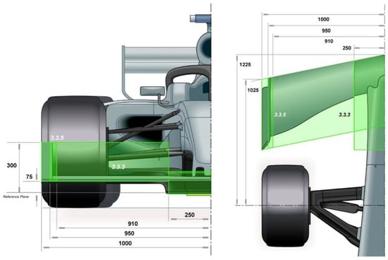
Figure A1.
2021 Regulations. Image extracted from the FIA regulations (Article 3.3 front wing [81]). The green areas are the size limits set by the FIA regulations. The non-dimensional numbers on the green areas stand for the subsection of Article 3.3 from the FIA regulations, in which additional information can be found.

On the sides, an endplate is defined from a 2D curved surface (virtual surface). This surface is constrained within a box between 910 mm and 950 mm from the car center line. The design should not create an angle greater than 15 from the center line of the car. Its surface must be continuous and uninterrupted, enclosing at least 95% of the virtual surface of the final plate. The end-plane surface can be offset from the virtual endplate surface by 10 mm in the first 150 mm of the plate and 6 mm in the rest of the endplate. In reality, the restrictions imposed make it difficult to deviate too far from the surface, as the front wing endplate is required to be at least 10 mm thick over its length, with a radius of at least 5 mm, to prevent damage to the tires of competitors. The baseplate is also defined by regulations. This can only protrude from the virtual surface up to 30 mm, while any geometry in this region cannot exceed 10 mm of thickness. The outer section of the baseplate may not exceed a height of 110 mm from the reference plane. Together, these rules almost completely define the shape of the endplate and baseplate, restricting design freedom and being barely optimisable.
Regarding the design of the profiles, the F1 rules give to designers and engineers restrictive rules. The front wing profiles are defined as a bodywork element that is constrained within the volume that extends from 250 mm to 950 mm from the car centreplane, and within the volume defined in Article 3.3.3 in the regulation [81], represented in Figure A1. Additionally, any intersection of these profiles with any longitudinal vertical plane may contain no more than five closed sections, each of which must contain a concave radius of curvature of maximum 50 mm. The regulation prohibits the visibility of the trailing edges of the wing elements when viewed from above. On the contrary, it requires the visibility of the trailing edges when viewed from below. The trailing edge limitations mean that the elements must be placed in series, without large overlaps. This rule is supported by a limit on element spacing between 5 mm and 15 mm, and from 400 mm up to 950 mm from the centerline, giving 150 mm of freedom to manipulate the Y250 vortex using the internal tips of the wing elements.
To avoid extreme angles in the profiles, the regulation also stipulates that the elements must join the virtual endplate surface at an angle of at least 15 from the horizontal, and at least one profile must be attached to the central mandatory section.
References
- Spalart, P.R.; Venkatakrishnan, V. On the role and challenges of CFD in the aerospace industry. Aeronaut. J. 2016, 120, 209. [Google Scholar] [CrossRef]
- Raheem, M.A.; Edi, P.; Pasha, A.A.; Rahman, M.M.; Juhany, K.A. Numerical study of variable camber continuous trailing edge flap at off-design conditions. Energies 2019, 12, 3185. [Google Scholar] [CrossRef]
- Biancolini, M.E.; Biancolini, C.; Costa, E.; Gattamelata, D.; Valentini, P.P. Industrial application of the meshless morpher RBF morph to a motorbike windshield optimisation. In Proceedings of the European Automotive Simulation Conference (EASC), Munich, Germany, 6–7 July 2009; pp. 6–7. [Google Scholar]
- Toet, W. Aerodynamics and aerodynamic research in Formula 1. Aeronaut. J. 2013, 117, 1–26. [Google Scholar] [CrossRef]
- Castro, X.; Rana, Z.A. Aerodynamic and structural design of a 2022 Formula One front wing assembly. Fluids 2020, 5, 237. [Google Scholar] [CrossRef]
- Patil, A.; Kshirsagar, S.; Parge, T. Study of front wing of formula one car using computational fluid dynamics. Int. J. Mech. Eng. Robot. Res. 2014, 3, 282. [Google Scholar]
- Mokhtar, W.; Durrer, S. A CFD analysis of a race car front wing in ground effect. In Proceedings of the ASEE North Central Section Conference, Mt Pleasant, MI, USA, 18–19 March 2016; pp. 18–19. [Google Scholar]
- Biancolini, M. Fluid structure interaction with RBF morph a generic Formula 1 front end. In Proceedings of the CAE Conference, Verona, Italy, 20–21 October 2011. [Google Scholar]
- Petrone, G.; Hill, C.; Biancolini, M.E. Track by track robust optimization of a F1 front wing using adjoint solutions and radial basis functions. In Proceedings of the 32nd AIAA Applied Aerodynamics Conference, Atlanta, GA, USA, 16–20 June 2014; p. 3174. [Google Scholar]
- Wade, A.; Keating, M.; Petrone, G. Shape optimisation for aerodynamic performance using adjoint methods. In Proceedings of the The International Vehicle Aerodynamics Conference, Prestwold, UK, 14–15 October 2014; Woodhead Publishing: Cambridge, UK, 2014; pp. 139–147. [Google Scholar]
- Ahlfeld, R.; Ciampoli, F.; Pietropaoli, M.; Pepper, N.; Montomoli, F. Data-driven uncertainty quantification for Formula 1: Diffuser, wing tip and front wing variations. Proc. Inst. Mech. Eng. Part D J. Automob. Eng. 2019, 233, 1495–1506. [Google Scholar] [CrossRef]
- Kalinowski, M.; Szczepanik, M. Aerodynamic shape optimization of racing car front wing. IOP Conf. Ser. Mater. Sci. Eng. 2021, 1037, 012058. [Google Scholar] [CrossRef]
- Melvin, A.; Martinelli, L. Aerodynamic shape optimization of multi-element airfoils in ground effect. In Proceedings of the 46th AIAA Aerospace Sciences Meeting and Exhibit, Reno, NV, USA, 7–10 January 2008; p. 327. [Google Scholar]
- Basso, M.; Cravero, C.; Marsano, D. Aerodynamic effect of the gurney flap on the front wing of a F1 car and flow interactions with car components. Energies 2021, 14, 2059. [Google Scholar] [CrossRef]
- Martins, D.; Correia, J.; Silva, A. The influence of front wing pressure distribution on wheel wake aerodynamics of a F1 car. Energies 2021, 14, 4421. [Google Scholar] [CrossRef]
- Guerrero, A.; Castilla, R. Aerodynamic study of the wake effects on a Formula 1 car. Energies 2020, 13, 5183. [Google Scholar] [CrossRef]
- Ravelli, U.; Savini, M. Aerodynamic simulation of a 2017 F1 car with open-source CFD code. J. Traffic Transp. Eng. 2018, 6, 155–163. [Google Scholar]
- Granados-Ortiz, F.-J.; Ortega-Casanova, J. Machine learning-aided design optimization of a mechanical micromixer. Phys. Fluids 2021, 33, 063604. [Google Scholar]
- Montomoli, F.; Carnevale, M.; D’Ammaro, A.; Massini, M.; Salvadori, S. Uncertainty Quantification in Computational Fluid Dynamics and Aircraft Engines; Springer: Berlin/Heidelberg, Germany, 2015. [Google Scholar]
- Skinner, S.N.; Zare-Behtash, H. State-of-the-art in aerodynamic shape optimisation methods. Appl. Soft Comput. 2018, 62, 933–962. [Google Scholar]
- Mirjalili, S. Particle swarm optimisation. In Evolutionary Algorithms and Neural Networks; Springer: Berlin/Heidelberg, Germany, 2019; pp. 15–31. [Google Scholar]
- Srinivas, N.; Deb, K. Multiobjective optimization using nondominated sorting in genetic algorithms. Evol. Comput. 1994, 2, 221–248. [Google Scholar] [CrossRef]
- Granados-Ortiz, F.-J.; Arroyo, C.; Pérez Arroyo, C.; Puigt, G.; Lai, C.-H.; Airiau, C. On the influence of uncertainty in computational simulations of a high-speed jet flow from an aircraft exhaust. Comput. Fluids 2019, 180, 139–158. [Google Scholar] [CrossRef]
- Fang, J.; Gao, Y.; Sun, G.; Zheng, G.; Li, Q. Dynamic crashing behavior of new extrudable multi-cell tubes with a functionally graded thickness. Int. J. Mech. Sci. 2015, 103, 63–73. [Google Scholar] [CrossRef]
- Ortega-Casanova, J. Application of cfd on the optimization by response surface methodology of a micromixing unit and its use as a chemical microreactor. Chem. Eng. Process. Process Intensif. 2017, 117, 18–26. [Google Scholar] [CrossRef]
- Klein, R.J.; Biserni, C.; Zinani, F.S.F.; Rocha, L.A.O. Constructal Design of tube arrangements for heat transfer to non-Newtonian fluids. Int. J. Mech. Sci. 2017, 133, 590–597. [Google Scholar] [CrossRef]
- Duchaine, F.; Morel, T.; Gicquel, L.Y.M. Computational-fluid-dynamics-based Kriging optimization tool for aeronautical combustion chambers. AIAA J. 2009, 47, 631–645. [Google Scholar]
- Zhang, Y.; Hu, S.; Wu, J.; Zhang, Y.; Chen, L. Multi-objective optimization of double suction centrifugal pump using Kriging metamodels. Adv. Eng. Softw. 2014, 74, 16–26. [Google Scholar] [CrossRef]
- Regis, R.G.; Shoemaker, C.A. Constrained global optimization of expensive black box functions using radial basis functions. J. Glob. Optim. 2005, 31, 153–171. [Google Scholar] [CrossRef]
- Bagheri, S.; Konen, W.; Bäck, T. Comparing kriging and radial basis function surrogates. In Proceedings of the 27th Workshop Computational Intelligence, Dortmund, Germany, 22–24 December 2017; pp. 243–259. [Google Scholar]
- Jakobsson, S.; Patriksson, M.; Rudholm, J.; Wojciechowski, A. A method for simulation based optimization using radial basis functions. Optim. Eng. 2010, 11, 501–532. [Google Scholar] [CrossRef]
- Biancolini, M.E. Fast Radial Basis Functions for Engineering Applications; Springer: Berlin/Heidelberg, Germany, 2017. [Google Scholar]
- Serani, A.; Pellegrini, R.; Wackers, J.; Jeanson, C.-J.; Queutey, P.; Visonneau, M.; Diez, M. Adaptive multi-fidelity sampling for CFD-based optimisation via radial basis function metamodels. Int. J. Comput. Fluid Dyn. 2019, 33, 237–255. [Google Scholar] [CrossRef]
- Rößger, P.; Richter, A. Performance of different optimization concepts for reactive flow systems based on combined CFD and response surface methods. Comput. Chem. Eng. 2018, 108, 232–239. [Google Scholar] [CrossRef]
- Qi, C.; Sun, Y.; Hu, H.; Wang, D.; Cao, G.; Yang, S. On design of hybrid material double-hat thin-walled beams under lateral impact. Int. J. Mech. Sci. 2016, 118, 21–35. [Google Scholar] [CrossRef]
- Rao, S.S. Engineering Optimization: Theory and Practice; John Wiley & Sons: Hoboken, NJ, USA, 2019. [Google Scholar]
- Glover, F. Future paths for integer programming and links to artificial intelligence. Comput. Oper. Res. 1986, 13, 533–549. [Google Scholar] [CrossRef]
- Abdel-Basset, M.; Abdel-Fatah, L.; Sangaiah, A.K. Metaheuristic algorithms: A comprehensive review. In Computational Intelligence for Multimedia Big Data on the Cloud with Engineering Applications; Elsevier: Amsterdam, The Netherlands, 2018; pp. 185–231. [Google Scholar]
- Wang, G.; Deb, S.; Coelho, L.D.S. Earthworm optimisation algorithm: A bio-inspired metaheuristic algorithm for global optimisation problems. Int. J. Bio-Inspired Comput. 2018, 12, 1–22. [Google Scholar] [CrossRef]
- Sun, J.; Lai, C.; Wu, X. Particle Swarm Optimisation: Classical and Quantum Perspectives; CRC Press: Boca Raton, FL, USA, 2016. [Google Scholar]
- Dey, N. Advancements in Applied Metaheuristic Computing; IGI Global: Hershey, PA, USA, 2017. [Google Scholar]
- Alsattar, H.A.; Zaidan, A.A.; Zaidan, B.B. Novel meta-heuristic bald eagle search optimisation algorithm. Artif. Intell. Rev. 2020, 53, 2237–2264. [Google Scholar] [CrossRef]
- Ortega-Casanova, J.; Castillo-Sanchez, S.I. On using axisymmetric turbulent impinging jets swirling as burger’s vortex for heat transfer applications. single and multi-objective vortex parameters optimization. Appl. Therm. Eng. 2017, 121, 103–114. [Google Scholar] [CrossRef]
- Ortega-Casanova, J.; Lai, C. Cfd study on laminar mixing at a very low reynolds number by pitching and heaving a square cylinder. Comput. Fluids 2018, 168, 318–327. [Google Scholar] [CrossRef]
- Ortega-Casanova, J.; Granados-Ortiz, F. Using machine-learning to speed-up optimisation in cfd: Designing a micromixer. In Proceedings of the APS Division of Fluid Dynamics Meeting Abstracts, Online, 22–24 November 2020; p. F13-005. [Google Scholar]
- Vasudev, K.L.; Sharma, R.; Bhattacharyya, S.K. A multi-objective optimization design framework integrated with CFD for the design of auvs. Methods Oceanogr. 2014, 10, 138–165. [Google Scholar] [CrossRef]
- Damavandi, M.D.; Forouzanmehr, M.; Safikhani, H. Modeling and Pareto based multi-objective optimization of wavy fin-and-elliptical tube heat exchangers using CFD and NSGA-II algorithm. Appl. Therm. Eng. 2017, 111, 325–339. [Google Scholar] [CrossRef]
- Wang, X.D.; Hirsch, C.; Kang, S.; Lacor, C. Multi-objective optimization of turbomachinery using improved NSGA-II and approximation model. Comput. Methods Appl. Mech. Eng. 2011, 200, 883–895. [Google Scholar] [CrossRef]
- Biancolini, M.E.; Viola, I.M.; Riotte, M. Sails trim optimisation using CFD and RBF mesh morphing. Comput. Fluids 2014, 93, 46–60. [Google Scholar] [CrossRef]
- Biancolini, M.E.; Costa, E.; Cella, U.; Groth, C.; Veble, G.; Andrejašič, M. Glider fuselage-wing junction optimization using CFD and RBF mesh morphing. Aircr. Eng. Aerosp. Technol. 2016, 88, 740–750. [Google Scholar] [CrossRef]
- Porziani, S.; Groth, C.; Waldman, W.; Biancolini, M.E. Automatic shape optimisation of structural parts driven by BGM and RBF mesh morphing. Int. J. Mech. Sci. 2021, 189, 105976. [Google Scholar] [CrossRef]
- Sovani, S.; Khondge, A. Scaling New Heights in Aerodynamics Optimization: The 50:50:50 Method; SAE Technical Paper (No. 2012-01-0174); SAE: Pittsburgh, PA, USA, 2012. [Google Scholar]
- Biancolini, M.E.; Capellini, K.; Costa, E.; Groth, C.; Celi, S. Fast interactive CFD evaluation of hemodynamics assisted by RBF mesh morphing and reduced order models: The case of aTAA modelling. Int. J. Interact. Des. Manuf. IJIDM 2020, 14, 1227–1238. [Google Scholar] [CrossRef]
- Dawes, W.N.; Meah, N.; Kudryavtsev, A.; Evans, R.; Hunt, M.; Tiller, P. Digital geometry to support a gas turbine digital twin. In AIAA Scitech 2019 Forum; AIAA: Reston, VA, USA, 2019; p. 1715. [Google Scholar]
- Kenway, G.; Mader, C.; He, P.; Martins, J. Effective adjoint approaches for computational fluid dynamics. Prog. Aerosp. Sci. 2019, 110, 100542. [Google Scholar] [CrossRef]
- Arora, J.S. Optimum design problem formulation. In Introduction to Optimum Design, 2nd ed.; Aurora, J.S., Ed.; Academic Press: San Diego, CA, USA, 2004; pp. 15–54. [Google Scholar]
- Fleischli, B.; Mangani, L.; Rio, A.; Casartelli, E. A discrete adjoint method for pressure-based algorithms. Comput. Fluids 2021, 227, 105037. [Google Scholar] [CrossRef]
- Biancolini, M.E. Mesh morphing and smoothing by means of radial basis functions (RBF): A practical example using fluent and RBF Morph. In Handbook of Research on Computational Science and Engineering: Theory and Practice; IGI Global: Hershey, PA, USA, 2012; pp. 347–380. [Google Scholar]
- ANSYS Release 15.0. ANSYS Fluent Adjoint Solver Manual. Original Typescript. 2013. Available online: https://www.scirp.org/(S(lz5mqp453ed%20snp55rrgjct55))/reference/referencespapers.aspx?referenceid=2869465 (accessed on 22 December 2022).
- Myers, R.H.; Montgomery, D.C. Response Surface Methodology: Process and Product in Optimization Using Designed Experiments; Taylor & Francis: Abingdon, UK, 1995. [Google Scholar]
- Deng, Y.; Lin, G.; Yang, X. Multifidelity data fusion via gradient-enhanced gaussian process regression. arXiv 2020, arXiv:2008.01066. [Google Scholar] [CrossRef]
- Baar, J.H.D.; Scholcz, T.P.; Verhoosel, C.V.; Dwight, R.P.; van Zuijlen, A.H.; Bijl, H. Efficient Uncertainty Quantification with Gradient-Enhanced Kriging: Applications in Fsi; ECCOMAS: Vienna, Austria, 2012. [Google Scholar]
- Jouhaud, J.; Sagaut, P.; Labeyrie, B. A kriging approach for CFD/wind-tunnel data comparison. J. Fluid Eng. 2006, 128, 847–855. [Google Scholar] [CrossRef]
- Williams, C.K.I.; Rasmussen, C.E. Gaussian Processes for Machine Learning; MIT Press: Cambridge, MA, USA, 2006; Volume 2. [Google Scholar]
- Lophaven, S.N.; Nielsen, H.B.; Sondergaard, J.; Dace, A. DACE: A Matlab Kriging Toolbox; Technical Report No. IMMTR-2002; Technical University of Denmark: Lyngby, Denmark, 2002; Volume 12. [Google Scholar]
- Deb, K.; Pratap, A.; Agarwal, S.; Meyarivan, T. A fast and elitist multiobjective genetic algorithm: NSGA-II. IEEE Trans. Evol. Comput. 2002, 6, 182–197. [Google Scholar] [CrossRef]
- Srinivas, N.; Deb, K. Multiobjective optimization using NSGA. Evol. Comput. 1995, 2. [Google Scholar]
- Tzanakis, A. Duct Optimization Using CFD Software ‘ANSYS Fluent Adjoint Solver’. 2014. Available online: https://hdl.handle.net/20.500.12380/202020 (accessed on 25 May 2021).
- Czerwiński, G.; Wołoszyn, J. Optimization of air cooling system using adjoint solver technique. Energies 2021, 14, 3753. [Google Scholar] [CrossRef]
- Sidik, N.A.C.; Yusof, S.N.A.; Asako, Y.; Mohamed, S.; Aziz, A. A short review on rans turbulence models. CFD Lett. 2020, 12, 83–96. [Google Scholar] [CrossRef]
- Menter, F. Zonal Two Equation k-w Turbulence Models for Aerodynamic Flows. In Proceedings of the 23rd Fluid Dynamics, Plasmadynamics, and Lasers Conference, Orlando, FL, USA, 6–9 July 1993. [Google Scholar]
- ANSYS Inc. Release 17.2. ANSYS Fluent User’s Guide; ANSYS: Canonsburg, PA, USA, 2016. [Google Scholar]
- JD Chaim Zerihan. An Investigation into the Aerodynamics of Wings in Ground Effect. Ph.D. Thesis, University of Southampton, Southampton, UK, 2001.
- Federation Internationale de l’Automobile (FIA). 2021 Formula 1 Sporting Regulations. Available online: https://www.fia.com/sites/default/files/2021_formula_1_sporting_regulations_-_iss_5_-_2020-12-16.pdf (accessed on 25 February 2022).
- Autosport. High-Downforce Tracks vs. Power Tracks in F1—Differences Explained. Available online: https://www.autosport.com/f1/news/high-downforce-track-vs-power-track-f1/6130208/ (accessed on 24 February 2022).
- Ladson, C.L.; Brooks, C.W., Jr.; Hill, A.S.; Sproles, D.W. Computer program to obtain ordinates for NACA airfoils. J. Stat. Phys. 1996, 104. [Google Scholar]
- Saffarian, M.R.; Jamaati, F.; Mohammadi, A.; Malekabad, F.G.; Ayoubloo, K.A. Investigating the entropy generation around an airfoil in turbulent flow. Aircr. Eng. Aerosp. Technol. 2020, 92, 1001–1017. [Google Scholar] [CrossRef]
- Rezaei, F.; Roohi, E.; Pasandideh-Fard, M. Stall simulation of flow around an airfoil using LES model and comparison of RANS models at low angle of attack. In Proceedings of the 15th Conference on Fluid Dynamics, Yerevan, Armenia, 14–18 July 2013; pp. 18–20. [Google Scholar]
- Sogukpinar, H.; Bozkurt, I. Implementation of different turbulence model to find proper model to estimate aerodynamic properties of airfoils. AIP Conf. Proc. 2018, 1935, 020003. [Google Scholar]
- Hafien, C.; Bourehla, A.; Bouzaiane, M. Passive separation control on a symmetric airfoil via elastic-layer. J. Appl. Fluid Mech. 2016, 9, 2569–2580. [Google Scholar] [CrossRef]
- Federation Internationale de l’Automobile (FIA). 2021 Formula 1 Technical Regulations. Available online: https://www.fia.com/regulation/category/110 (accessed on 28 February 2021).
Disclaimer/Publisher’s Note: The statements, opinions and data contained in all publications are solely those of the individual author(s) and contributor(s) and not of MDPI and/or the editor(s). MDPI and/or the editor(s) disclaim responsibility for any injury to people or property resulting from any ideas, methods, instructions or products referred to in the content. |
© 2023 by the authors. Licensee MDPI, Basel, Switzerland. This article is an open access article distributed under the terms and conditions of the Creative Commons Attribution (CC BY) license (https://creativecommons.org/licenses/by/4.0/).

