Abstract
A significant number of people in the world suffer from limb losses, while prosthesis is the hopeful way to help the amputees back to normal life. Recently, the most popular control method used in intelligent prosthesis is FSM-IC (finite state machine with impedance control), which requires a significant amount of manual parameter adjustments to achieve a good model compensation in a discrete way. Taking the lower-limb prosthesis as the research object, this paper applies an LWPR (locally weighted projection regression) model to learn the dynamic model of a prosthesis in real time in order to achieve a better model compensation in a continuous way and propose scientific experimental schemes to verify the control method. First, the basic control framework of lower-limb prosthesis is given. Then, the control law is derived on the basis of model building and LWPR’s addition. Finally, the proper experimental schemes are designed to carry out the control method effectively in a safe way. The experimental results show that the control law with the LWPR model can greatly improve the tracking performance during the swing phase and obtain rather good compliance during the stance phase. Moreover, the results also indicate that the LWPR model can approximate the dynamic model online. This method is hoped to be extended to more applications and fields.
1. Introduction
Amputation of the lower limbs is becoming more and more common due to traffic accidents, diabetes, congenital diseases, tumors [1], etc. Lower-limb losses will lead to limited mobility and psychological burden. In order to restore the mobility and return to normal life, the prosthetic technique is the option of most amputees. Most commercial prostheses are passive because they are cheap and simple in structure. However, walking with a passive prothesis will consume more energy [2] than the able-bodied and the asymmetry may cause secondary damage [3]. Therefore, the research on intelligent prosthesis has become more popular due to its potential in speed switch and adaptation in different terrains.
The general control frameworks of intelligent lower-limb prosthesis are hierarchical into high-level controller, mid-level controller, and low-level controller [4]. The high-level controller aims at human intention recognition including locomotion mode classification, gait parameter determination, and gait phase determination. The low-level controller makes the actuators output the desired torques. The mid-level controller pays attention to intent-to-state conversion and achieves a good interaction between human and prosthesis. For now, a significant amount of control methods have been proposed. Some (e.g., CLME (complementary limb motion estimation) [5] and echo control [6]) collect the kinematic data of the sound leg to complete the auxiliary control of the prosthesis. Model-based methods [7,8] build the dynamic model or human neuromuscular system to generate the joint torques. Phase-based methods introduce continuous gait phase variable to calculate joint trajectory which is followed by the controller. Refs. [9,10] adopt the COP as a mechanical representation of the gait cycle phase, while [11] extracts proper phase variables from the motion information of the thigh. Ref. [12] uses discrete Fourier transform (DFT) to characterize the desired periodic joint trajectories as functions of gait phase. Refs. [13,14,15] apply FSM–IC (finite state machine with impedance control), which divides a complete gait into several gait stages. In each gait stage, virtual spring damping systems are used to model the impedance of different joints and a significant amount of impedance parameters need to be adjusted for a good model compensation. Furthermore, [16] automatically tunes the impedance parameters by the ADP (approximate dynamic programming) approach. The above control methods mainly consider the tracking performance of joints’ trajectories while the performance of compliance is not well considered. To achieve both good compliance and tracking performance for intelligent lower-limb prosthesis, this paper mainly focuses on the mid-level controller to compute the desired torques of knee and ankle.
For an intelligent lower-limb prosthesis, its control goal is improving the tracking performance during the swing phase and compliance during the support phase, which conforms to the human motion mechanism. In order to achieve the above goal, we need to compute the model compensation as a feedforward item by adjusting impedance parameters or modeling. FSM-IC methods adjust impedance parameters and model compensation in a discrete way. Due to uncertain joint friction, model error, and other possible factors, modeling methods can achieve good results in simulation but face the problems of disturbance estimation and real-time model compensation in the real world. Ref. [17] enhances compliance by using the LWPR method [18] to fit the dynamic model. However, the control strategy in [17] is only validated on a simulated biped walker rather than a real human–machine system. Here, we have achieved the migration process from a simulation of the real world by combining the LWPR model and PD controller. The contributions of this paper are listed below: (1) Through theoretical analysis, the control law is obtained and the training method is determined (the LWPR model is only trained in the swing phase); (2) According to the complexity of the model from simple to complex, four experiments are designed to gradually verify the feasibility of the proposed control method and ensure the safety of people; (3) As for prosthesis application, the LWPR model has the ability to rapidly fit the dynamic model in real time, which is input into the controller as a real-time model compensation; (4) Compared with previous works, there are less parameters to be adjusted. (5) The real-time learning of the LWPR model can adapt to the model change.
2. Materials and Methods
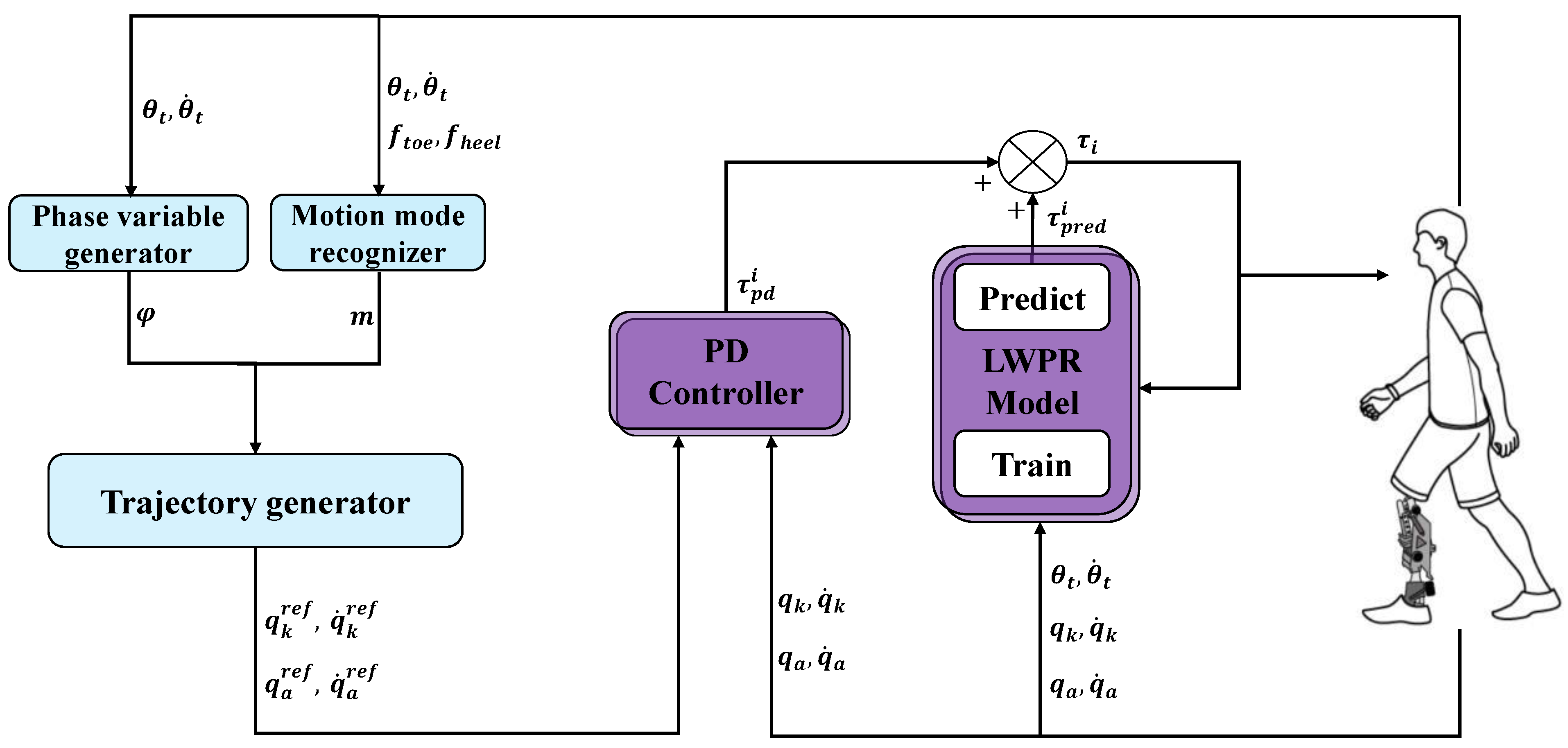
The control framework used in this paper is shown in Figure 1, and relevant variables are shown in Figure 2. Under this control framework, [17] completes a simulation experiment and finds a good result. In order to achieve the subjects’ walking experiment on the treadmill safely and successfully, there are still significant amounts of analysis and tests to conduct. Each part of the control framework will be introduced below.

Figure 1.
The control framework of intelligent lower-limb prosthesis. The blue parts are the high-level and mid-level controller, which aims at human intention recognition and joint trajectory planning. The purple parts are the main research subjects in this paper.
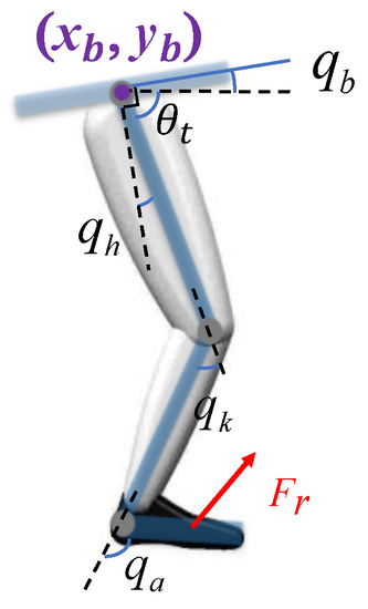
Figure 2.
The simplified lower-limb prosthesis model.
2.1. Phase Variable Selection
We install the IMU (inertial measurement unit) on the part where the prosthesis is fixedly connected with the injured thigh of the transfemoral amputee. On the one hand, the motions of the injured thigh can reflect the amputees’ motion intention. On the other hand, the sensors are required to be on-board (installed on the prosthesis rather than on the people), which can reduce system complexity and improve convenience. The installed IMU can detect the movement of the thigh in real time with a frequency of 100 Hz (sampling time ). The real-time gait phase is obtained through thigh movement [11] when the amputees walk with periodic gaits (e.g., level walking, stair ascent, stair descent, ramp ascent, ramp descent). The real-time gait phase is computed as
where and are thigh angular velocity and thigh angle, respectively, and and are the filtered and normalized thigh angular velocity and thigh angle, respectively [15].
2.2. Motion Mode Recognizer
Different motion modes have different joint reference trajectories. This module aims at classifying the locomotion mode according to the sensors’ information. However, the focus of this paper is not on the high-level controller. Therefore, we set our locomotion mode as level walking for the convenience of narration.
2.3. Reference Trajectory Generation
For level walking, which corresponds to periodic motion, we use Fourier series to describe the reference trajectory.
where represents the controlled joint, is the offset term, and is the amplitude of the -th cosine harmonic component. and are obtained by discrete Fourier transform of the collected joint angle data set off-line.
2.4. Controller Design
We simplify the lower-limb prosthesis to a three-joint manipulator with a floating base (Figure 2). Then, its dynamic equation can be written as
where is the inertia matrix, is the centrifugal and Coriolis force term, is the gravity term and is the projection of ground reaction force (GRF) acting on the foot into forces acting in the degrees of freedom (DOFs). and are defined as
where , , and are forces and torque on the sagittal plane of floating base. , and are the three DOFs of floating base. is the joint angle vector and is the torque input vector. For knee and ankle, their dynamic equations are
where and are the projection of GRF acting on the foot into forces acting in the knee and ankle.
Here, we intend to use the LWPR model to fit the lower-limb prosthesis model. The LWPR model is of multi-input and single output. For each joint
where is according to the dynamic model in Table A1 of Appendix A and . We use LWPR models [2] to approximate
where is the input vector of the LWPR model (variables in can be obtained from the thigh IMU and joint encoders). When is given, every linear model calculates a predicted value , and the normalized weighted mean of all linear models are the output of the LWPR model. , , and are the angular velocity of thigh IMU, knee, and ankle at the last moment. are Gaussian functions called RFs (receptive fields) which are computed as seen in Equation (8), is the number of local linear models, and is the error between the real dynamic model and the LWPR model.
where is the distance metric and are the centers of RFs.
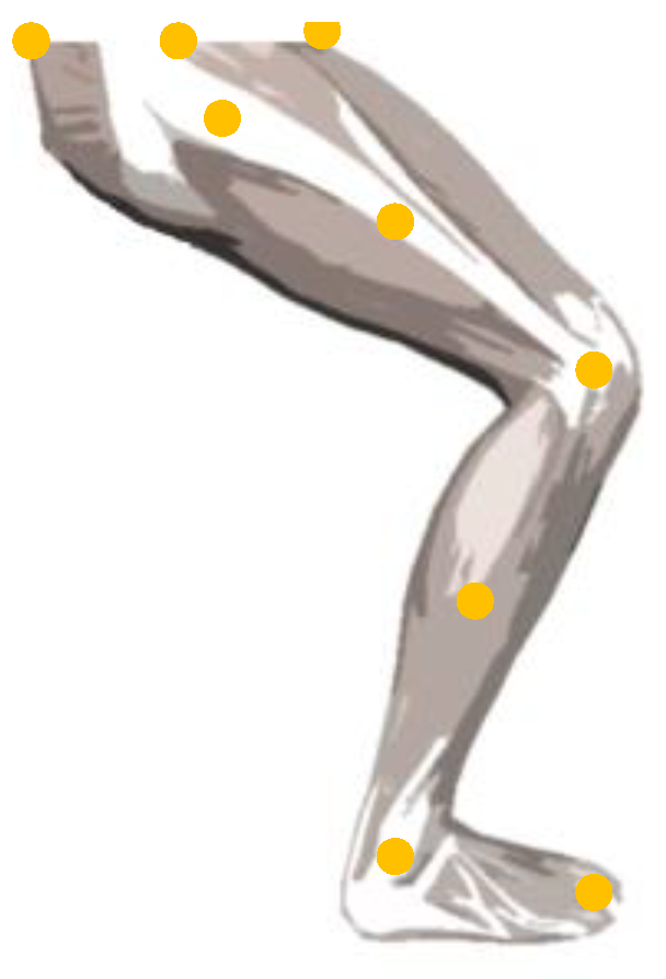
Is the given input sufficient for the fitting? We record the coordinates of motion capture markers (Figure 3) [19] and thigh IMU data when the subject walks on the treadmill with a 3 km/h speed and computes related variables by OpenSim [20].

Figure 3.
The markers of motion capture system.
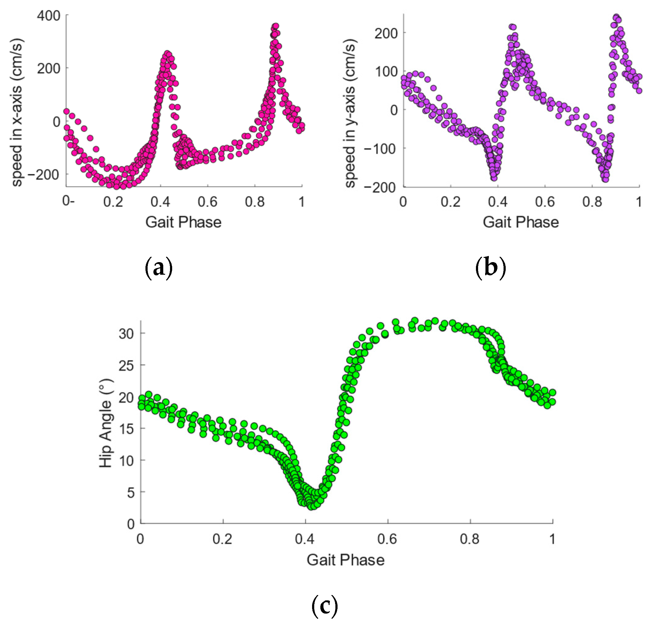
We can obtain the gait phase from and , and it can be concluded from the plots in Figure 4 that , , and are the functions of gait phase when the subject is walking at a constant speed, which means that
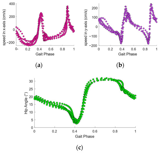
Figure 4.
(a) Scatter plot of and gait phase. (b) Scatter plot of and gait phase. (c) Scatter plot of hip joint angle and gait phase. All those points are computed by motion capture data during walking on the treadmill with a speed of 3 km/h.
According to relationships shown in Figure 2 and speed calculation formula, we have
where , , and can be computed by . The derivatives of , , and also are the functions of gait phase according to Equation (11).
where . When the subject walks with a constant speed, can be regarded as a constant and .
Thus, it is proved that can be determined by when the subject moves at a constant speed.
The control laws adopted are as follows:
where , and and are the stiffness coefficient and damping coefficient, respectively.
Let us combine Equations (6), (7), and (12):
- (1)
- During swing phase
When the lower limb is in the swing phase, there is no contact between the foot and the ground, so the GRF is zero. Therefore, it can be assumed that
Therefore, Equation (13) can be simplified as
The solution of the differential Equation (15) is
where . When , . The author of [17] shows that the LWPR model can converge to a low error with proper model parameters as well as applied and continuous real-time learning. Equation (16) indicates that high stiffness and low damping can improve convergence speed.
- (2)
- During stance phase
GRF acts on the prosthesis when the lower limb is in the stance phase, and we have
where is the external torque on joint. Therefore, we have
Equation (18) shows that when , the joint is of the dynamic characteristics of the spring damping system. It can help to adjust the relationship between external torque and joint motion, which is called compliance control.
2.5. Learning Policy of LWPR Model
2.5.1. LWPR Model Configuration
A significant number of parameters in the LWPR model need to be adjusted to improve the fitting accuracy and speed. is the initial value of (set initial distance metric where is n-dimensional identity matrix and is the number of the LWPR model’s input variables); init_alpha is the learning rate of updating ; w_gen is a threshold to determine when to create a new receptive filed. More detailed setup and initialization of parameters can be found in the library [21]. Table 1 reports some of the model parameters’ values in this paper.

Table 1.
Model parameters of LWPR set in the paper.
2.5.2. Model Learning Policy
According to Equation (7), the LWPR model is intended to fit the internal dynamic model of the joint. The internal dynamic model does not include the external torque (external torque mainly comes from the GRF during walking). Therefore, the LWPR model only trains itself when there are not any external forces while its training input is real-time measurable states of the internal dynamic model and its training output is the real-time motor output torque. Before the LWPR model is added to the control law as a model compensation, it should be trained for a while to approach the internal dynamic model when there are no external forces.
The experiments in this paper all follow the learning policy of the LWPR model above.
3. Results
According to the complexity of the model from simple to complex, four experiments are designed to gradually verify the feasibility of the proposed control method and ensure the safety of people. The single motor (dynamic model of one-dimension) experiment aims at testing the LWPR model’s astringency. Considering more complex situations (the centrifugal and Coriolis force term, the gravity term, and higher dimension inputs are added into the dynamic model), a hanging up experiment is intended for further testing the capability of LWPR. After wearing the prosthesis, the real dynamic model will change due to human’s involvement. By the leg swinging experiment, the LWPR model is closer to the changed model. When subjects walk on the treadmill, the GRF will appear. The walking experiment is the final test to verify the whole prosthesis control system’s performance including tracking performance and compliance.
All the motors used in above four experiments are the same. The motors’ reduction ratio is 1:50 and their angle and angular speed are sampled with a frequency of 100 Hz. Except the single motor experiment, the thigh angle and angular velocity in the sagittal plane are recorded with a frequency of 100 Hz.
3.1. Single Motor Experiment
The control method is tested with one motor which is laid flat on the table. In the first 30 s, the PD controller is applied and the LWPR model is only learning while the motor input torque . The training inputs of the LWPR model are the angle and angular speed of the motor, and the model’s training output is . After 30 s, the LWPR model’s output is added into the motor input torque . We calculate the RMSE to assess the tracking performance.
In this paper, . The experiment result is shown in Figure 5. In pure PD mode, the single motor cannot keep up with the sinusoidal curve (in fact, [22] shows that the PID controller cannot track a sine signal with zero error) When the LWPR model is used, the tracking error decreases by about four times and almost reaches a stable value.
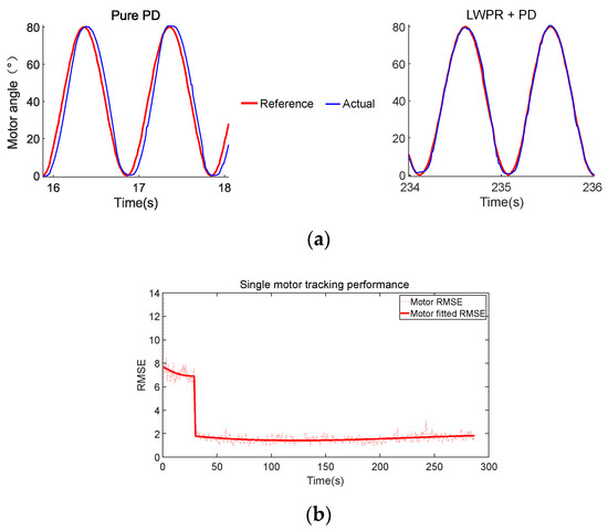
Figure 5.
(a) Motor’s position tracking under different modes. (b) Tracking performance of single motor.
3.2. Hanging Up Experiment
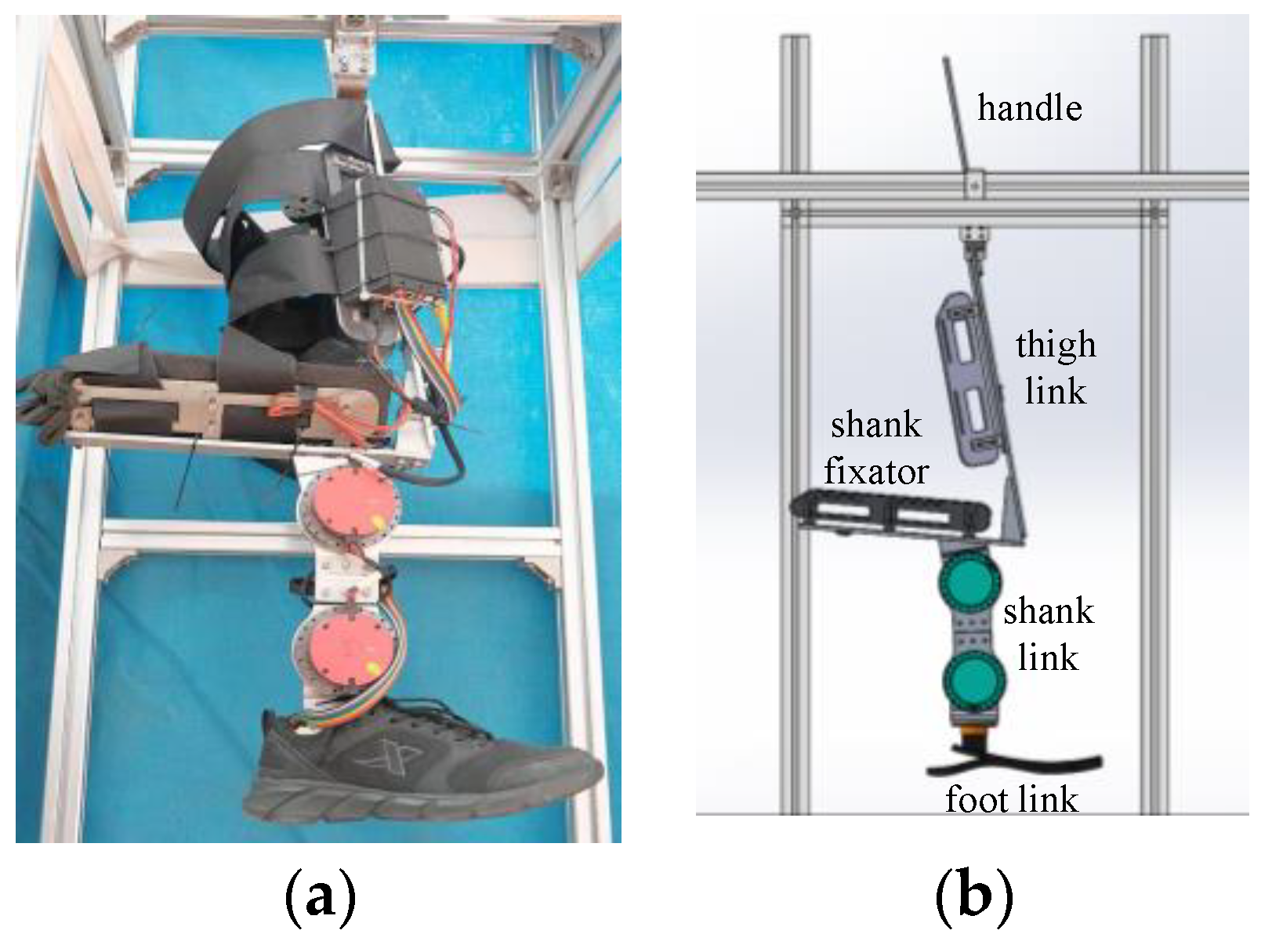
The control framework shown in Figure 1 is used in the experiment. We hung the lower-limb prosthesis on a fixed frame (Figure 6). We simulated human thigh movement by swinging the handle to generate phase firstly. Then, we use Fourier series to compute the reference trajectory.

Figure 6.
(a) Lower-limb prosthesis designed for healthy subjects. (b) Mechanical structure diagram of lower-limb prosthesis.
In the first 30 s. Step 1: only the PD controller is applied, while the LWPR model is trained but not applied during this time. The training input of the LWPR model is the vector , and the training output is .
After 30 s. Step 2: we add the predicted value of the LWPR model to the motor input torques. At this stage, the training input of the LWPR model is the vector , and the training output is the . Then, the value of and will be decreased to and .
Figure 7 reports our results. The results show that under LWPR+PD mode, the RMSE of knee angle reduced by five times and the RMSE of ankle angle remain almost unchanged. We hypothesize that the reason for this is that during the experiment, the ankle torque is small and the error of the LWPR model are at the same level, which leads to no improvement of tracking performance.
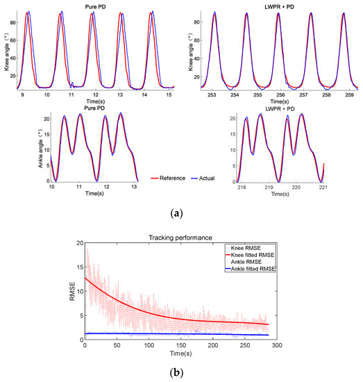
Figure 7.
(a) Knee and ankle position tracking under different modes. (b) Tracking performance of knee and ankle.
In this experiment, and of knee and ankle are, respectively,
The decrease in the knee’s RMSE indicates that the LWPR model provides model compensation but there is still some which is not compensated for. After model compensation, the PD controller can focus more on the error control rather than the uncertain model compensation.
3.3. Leg Swinging Experiment
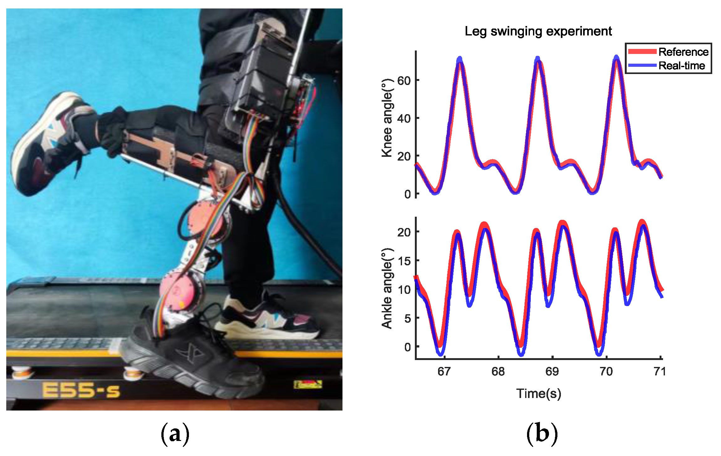
In this experiment, the subject is required to wear the lower-limb prosthesis, which will change the dynamic model indeed. In order to ensure the subjects’ safety, we need to further train our LWPR model to approach the changed model. The experiment is set as follows: The healthy leg stands still and the other leg swings in the air to train the LWPR model for a few minutes (Figure 8a) until the tracking performance is better (Figure 8b). The trained LWPR model in the hanging up experiment is used as the initial model here. Only step 2 in the hanging up experiment is applied in the training process.

Figure 8.
(a) The platform of leg swinging experiment. (b) Leg swinging experiment results.
3.4. Walking Experiment
Based on the LWPR model trained in 3.3 as the initial LWPR model, the subjects are required to walk on the treadmill with a comfortable velocity (3 km/h in our experiment). Only step 2 in the hanging up experiment is applied in the training process.
From the experimental results in Figure 9, during the swing phase, we have a rather good tracking performance on knee and ankle position. During the stance phase, the tracking errors of knee and ankle increase because the external torques appear, which proves that the model compensation of LWPR is effective and that the proposed method can bring high compliance to the prosthesis. However, at the beginning of the stance phase, the tracking errors have not been increased immediately, which indicates that there are still errors between the LWPR model and the real dynamic model.
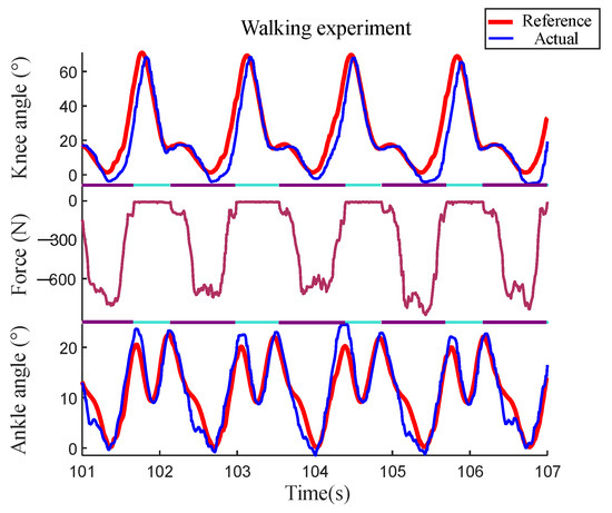
Figure 9.
The results of walking experiment on treadmill. Force is the value of GRF and the downward direction is positive. The stance phase is marked with purple horizontal bars while the swing phase is marked with blueish green bars.
According to Equation (18), the smaller is, the better the compliance and the LWPR model. The good tracking performance and high compliance prove that the LWPR model can fit the real dynamic model in real time.
We capture a one-minute Video S1 of a walking experiment and upload it. According to the subjects’ feeling, the impact force between prosthesis and ground is similar to the healthy side, and there is little lag in the swing of the lower-limb prosthesis. Due to the influence of the shank which is on the fixator, the upper body needs to be forward to keep balance. Moreover, the height of the knee joints of both legs is also different due to the difference between healthy people and disabled people. Next, we will improve the mechanical structure and invite the transfemoral amputees to participate in the experiment.
4. Discussion
Through theoretical derivation, the control law is given and the LWPR model is applied. In order to verify the LWPR model’s effectiveness (whether model compensation can be achieved) and test the performance of the prosthesis control system, we plan our experiments step by step in a scientific way. The results of the walking experiment show that our method can improve tracking performance during swing phase and bring good compliance during the stance phase, while these two performances are exactly what the lower-limb prosthesis control system is seeking. This paper’s contribution can be summarized as follows.
First, this paper proposes the control law of lower-limb prosthesis by theoretical derivation. According to the control law, we need to train the LWPR model only during the swing phase to obtain the performances we want. If we train the LWPR model during the stance phase, the external force torque will be included in the LWPR model and the compliance will not be shown during the stance phase.
Second, a scientific experimental scheme is proposed to initialize the LWPR model. From simulation to experiment is a difficult process, especially when people are involved. A series of experiments seems a little redundant, but they help establish the confidence of the subjects and ensure safety. In human–computer interaction, it is crucial to consider human factors both physically and psychologically.
Finally, good performances in the walking experiment prove that the proposed control method is good in use and that the LWPR model can learn the dynamic model in real-time to achieve a good model compensation.
5. Conclusions
This paper’s control method preliminarily shows that the LWPR model is an effective tool for prosthesis application. In high-dimensional space, LWPR greatly improves its computational efficiency by performing linear approximate fitting locally [18]. Due to measurement error and limited measurement information, the fitting error still exists. In the future, the follow points need to be studied further. (1) How to measure the error of the LWPR model and control it? (2) When real dynamic model changes (such as speed changes), how long does it take to for the LWPR model to learn and how to improve learning efficiency? (3) How to use prior knowledge in the LWPR model? (4) Are more sensors necessary? If necessary, which sensors are added? To improve the performance of lower-limb prosthesis, those problems above are what we will study next.
Supplementary Materials
The following supporting information can be downloaded at: https://www.mdpi.com/article/10.3390/machines11020186/s1, Video S1: Walking Experiment.
Author Contributions
Conceptualization, Y.L. and H.A.; methodology, Y.L. and H.A.; software, Y.L.; validation, Y.L., H.A., and H.M.; formal analysis, Y.L.; data curation, Y.L.; writing—original draft preparation, Y.L.; writing—review and editing, H.A., H.M., and Q.W.; visualization, Y.L.; supervision, H.A., H.M., and Q.W.; project administration, H.A.; funding acquisition, H.A., H.M., and Q.W. All authors have read and agreed to the published version of the manuscript.
Funding
This research was funded by the project of the National Key Research and Development Program of China, grant number (2018YFC2001304).
Informed Consent Statement
Not applicable.
Data Availability Statement
Not applicable.
Conflicts of Interest
The authors declare no conflict of interest.
Appendix A
The simplified model of lower-limb prosthesis has been built before. Its dynamic equation is shown in Equation (3). We define
The values of parameters in the dynamic equation are given in Table A1. , , and are the masses of floating base, thigh, shank, and foot, respectively; , , and are the moment of inertia of floating base, thigh, shank, and foot, respectively; and are the length of thigh and shank, respectively; is the length from hip joint to mass center of thigh; is the length from knee joint to mass center of shank; is the length from ankle joint to mass center of foot, and the definitions of the rest of the variables are shown in Figure 2.

Table A1.
The values of parameters in dynamic equation.
Table A1.
The values of parameters in dynamic equation.
| Parameters | Value |
|---|---|
| 0 | |
| 0 | |
| 0 | |
References
- Sagawa, Y.; Turcot, K.; Armand, S.; Thevenon, A.; Vuillerme, N.; Watelain, E. Biomechanics and physiological parameters during gait in lower-limb amputees: A systematic review. Gait Posture 2011, 33, 511–526. [Google Scholar] [CrossRef] [PubMed]
- Ettema, S.; Kal, E.; Han, H. Energy cost of walking in people after lower limb amputation: A systematic review and meta-analysis. Gait Posture 2020, 81, 89–90. [Google Scholar] [CrossRef]
- Robert, G.; Kerry, A.; Julie, C.; Jennifer, K.; Mariah, R. Review of secondary physical conditions associated with lower-limb amputation and long-term prosthesis use. J. Rehabil. Res. Dev. 2008, 45, 15–30. [Google Scholar]
- Tucker, M.R.; Olivier, J.; Pagel, A.; Bleuler, H.; Bouri, M.; Lambercy, O.; del R Millán, J.; Riener, R.; Vallery, H.; Gassert, R. Control strategies for active lower extremity prosthetics and orthotics: A review. J. NeuroEngineering Rehabil. 2015, 12, 1. [Google Scholar] [CrossRef] [PubMed]
- Pfeifer, S.; Allery, H.; List, R.J.; Perreault, E.J.; Riener, R. Finding Best Predictors for the Control of Transfemoral Prostheses. 2010. Available online: https://www.automed2010.ethz.ch/tagungsband/sitzung5_beitrag4_pfeifer.pdf (accessed on 26 January 2023).
- Wang, W.; Li, J.; Li, W.; Sun, L.N. An Echo-Based Gait Phase Determination Method of Lower Limb Prosthesis. Mechatron. Intell. Mater. III PTS 1-3 2013, 706, 629–634. [Google Scholar] [CrossRef]
- Lyu, Y.; Fang, H.; Xu, J.; Jianmin, M.; Qining, W.; Xiaoxu, Z. Dynamic Modeling and Analysis of the Lower Limb Prosthesis with Four-bar Linkage Prosthetic Knee. Chin. J. Theor. Appl. Mech. 2020, 52, 1157–1173. [Google Scholar]
- Thatte, N.; Geyer, H. Toward Balance Recovery with Leg Prostheses Using Neuromuscular Model Control. IEEE Trans. Biomed. Eng. 2016, 63, 904–913. [Google Scholar] [CrossRef] [PubMed]
- Gregg, R.D.; Sensinger, J.W. Towards Biomimetic Virtual Constraint Control of a Powered Prosthetic Leg. IEEE Trans. Control Syst. Technol. 2014, 22, 246–254. [Google Scholar] [CrossRef] [PubMed]
- Gregg, R.D.; Lenzi, T.; Hargrove, L.J.; Sensinger, J.W. Virtual Constraint Control of a Powered Prosthetic Leg: From Simulation to Experiments with Transfemoral Amputees. IEEE Trans. Robot. 2014, 30, 1455–1471. [Google Scholar] [CrossRef] [PubMed]
- Quintero, D.; Lambert, D.J.; Villarreal, D.J.; Gregg, R.D.; Department of Mechanical Engineering. Real-Time continuous gait phase and speed estimation from a single sensor. In Proceedings of the Conference on Control Technology and Applications (CCTA), Maui, HI, USA, 27–30 August 2017. [Google Scholar]
- Quintero, D.; Villarreal, D.J.; Lambert, D.J.; Kapp, S.; Gregg, R.D. Continuous-Phase Control of a Powered Knee–Ankle Prosthesis: Amputee Experiments Across Speeds and Inclines. IEEE Trans. Robot. 2018, 34, 686–701. [Google Scholar] [CrossRef] [PubMed]
- Shultz, A.H.; Goldfarb, M. A Unified Controller for Walking on Even and Uneven Terrain with a Powered Ankle Prosthesis. IEEE Trans. Neural Syst. Rehabil. Eng. 2018, 26, 788–797. [Google Scholar] [CrossRef] [PubMed]
- Culver, S.; Bartlett, H.; Shultz, A.; Goldfarb, M. A Stair Ascent and Descent Controller for a Powered Ankle Prosthesis. IEEE Trans. Neural Syst. Rehabil. Eng. 2018, 26, 993–1002. [Google Scholar] [CrossRef] [PubMed]
- Ledoux, E.D.; Goldfarb, M. Control and Evaluation of a Powered Transfemoral Prosthesis for Stair Ascent. IEEE Trans. Neural Syst. Rehabil. Eng. 2017, 25, 917–924. [Google Scholar] [CrossRef] [PubMed]
- Wen, Y.; Si, J.; Brandt, A.; Gao, X.; Huang, H.H. Online Reinforcement Learning Control for the Personalization of a Robotic Knee Prosthesis. IEEE Trans. Cybern. 2019, 50, 2346–2356. [Google Scholar] [CrossRef] [PubMed]
- Heins, S.; Tolu, S.; Ronsse, R. Online Learning of the Dynamical Internal Model of Transfemoral Prosthesis for Enhancing Compliance. IEEE Robot. Autom. Lett. 2021, 6, 6156–6163. [Google Scholar] [CrossRef]
- Vijayakumar, S.; D’Souza, A.; Schaal, S. Incremental Online Learning in High Dimensions. Neural Comput. 2005, 17, 2602–2634. [Google Scholar] [CrossRef]
- Camargo, J.; Ramanathan, A.; Flanagan, W.; Young, A. A comprehensive, open-source dataset of lower limb biomechanics in multiple conditions of stairs, ramps, and level-ground ambulation and transitions. J. Biomech. 2021, 119, 110320. [Google Scholar] [CrossRef] [PubMed]
- Camargo, J.; Ramanathan, A.; Csomay-Shanklin, N.; Young, A. Automated gap-filling for marker-based biomechanical motion capture data. Comput. Methods Biomech. Biomed. Eng. 2020, 23, 1180–1189. [Google Scholar] [CrossRef] [PubMed]
- Klanke, S.; Vijayakumar, S.; Schaal, S. A Library for Locally Weighted Projection Regression. J. Mach. Learn. Res. 2008, 9, 623–626. [Google Scholar]
- Alejandro, G.Y.; Francisco, D.F.; Jesus, D.G.; Oscar, L. Effects of Discretization Methods on the Performance of Resonant Controllers. IEEE Trans. Power Electron. 2010, 25, 1692–1712. [Google Scholar]
Disclaimer/Publisher’s Note: The statements, opinions and data contained in all publications are solely those of the individual author(s) and contributor(s) and not of MDPI and/or the editor(s). MDPI and/or the editor(s) disclaim responsibility for any injury to people or property resulting from any ideas, methods, instructions or products referred to in the content. |
© 2023 by the authors. Licensee MDPI, Basel, Switzerland. This article is an open access article distributed under the terms and conditions of the Creative Commons Attribution (CC BY) license (https://creativecommons.org/licenses/by/4.0/).

