Optimal Scheduling of Photovoltaic Generators in Asymmetric Bipolar DC Grids Using a Robust Recursive Quadratic Convex Approximation

Abstract

This paper presents a robust quadratic convex model for the optimal scheduling of photovoltaic generators in unbalanced bipolar DC grids. The proposed model is based on Taylor’s series expansion which relaxes the hyperbolic relation between constant power terminals and voltage profiles. Furthermore, the proposed model is solved in the recursive form to reduce the error generated by relaxations assumed. Additionally, uncertainties in PV generators are considered to assess the effectiveness of the proposed recursive convex. Several proposed scenarios for the numerical validations in a modified 21-bus test system were tested to validate the robust convex model’s performance. All the simulations were carried out in the MATLAB programming environment using Yalmip and Gurobi solver. Initially, a comparative analysis with three combinatorial optimization methods under three PV generation scenarios was performed. These scenarios consider levels of 0, 50, and 100% capacity of the PV systems. The results demonstrate the effectiveness of the proposed recursively solved convex model, which always achieves the global optimum for three levels of capacity of the PV generators, with solutions of $95.423$ kW, $31.525$ kW, and $22.985$ kW for 0%, 50%, and 100% of the capacity PV rating, respectively. In contrast, the combinatorial optimization methods do not always reach these solutions. Furthermore, the power loss for the robust model is comparable to the deterministic model, increasing by 1.65% compared to the deterministic model.

1. Introduction

1.1. General Context

Electrical distribution networks are extensions of wires along cities and countries that provide electricity service to hundreds of thousands of end-users at medium- and low-voltage levels [1,2]. These grids are typically constructed using AC technologies and three-phase configurations. Nevertheless, the significant advances in power electronics, renewable energy technologies, and energy storage technologies have transformed electrical networks from passive systems to active distribution networks [3]. The active concept in these networks is related to the possibility of self-management and bidirectional energy flows [4,5]. In addition, a new paradigm for the operation of active distribution networks based on DC technologies has seen rapid growth, because these DC networks have the main advantage that they are easily controllable and do not require control for frequency or reactive power [6]. DC distribution is attracting more attention in industries and academia since they can easily integrate generation and energy storage (i.e., photovoltaics and batteries) that work directly using DC signals. This implies that some conversion stages can be eliminated, making these networks more reliable and efficient [7].

The usage of DC technology for providing electricity service at medium and low voltage levels can be implemented using two main configurations [8]. The first topology corresponds to the monopolar DC network configuration, which uses two wires, one of the sets with a $+V_{DC}$ voltage and the another one that works as the return cable and is solidly grounded as the load point [9]. The second topology adds a new wire to the monopolar configurations. It is referred to as the bipolar DC system, where there are two poles set with voltages $\pm V_{DC}$ as well as the return wire, with the same function. In the case of bipolar DC distribution networks, the return wire can be solidly grounded or not [10,11]. The main advantage of bipolar systems is that with 33% additional investment, it is possible to duplicate the number of users connected to these grids, with the possibility of connecting multiple bipolar users that receive twice the voltage magnitude at their terminals [12].

1.2. Motivation

The analysis of bipolar DC networks requires the development of new control and optimization methods to manage all the devices connected to them in order to maximize efficiency, reliability, and security [7]. This research is motivated by studying unbalanced monopolar DC networks, from an optimization point of view [11]. The optimization in electrical distribution networks is a necessity for all systems that include distributed energy resources and demand variations during the day, since it is necessary to determine the best power injections for power plants and the best energy storage profiles for batteries by ensuring that all the technical conditions of the distribution network are maintained, i.e., voltage regulation, thermal capabilities in conductors, and generation bounds, among others [13]. In this study, considering the growing relevance of bipolar DC distribution networks we have been motivated to propose a robust optimization methodology for efficiently dispatching photovoltaic (PV) plants in bipolar DC networks from the convex optimization point of view [14]. This robust optimization approach includes uncertainties regarding the expected power output in the generation profile.

1.3. Literature Review

In the specialized literature, multiple methods have been proposed to solve the optimal power flow (OPF) in bipolar DC networks with asymmetric loads. An OPF model based on measurements of voltages and currents of bipolar DC grids was proposed in [10]. This model employed a non-convex objective function with a bilinear form generating a relationship between the objective function and constraints with a weak duality. This weakness was solved using locational marginal prices to convert the proposed bilinear model into a two-step linear problem. In [15], a model for solving the OPF problem in asymmetric bipolar DC grids was described. The objective function of this model was to reduce the congestion in the lines and unbalance of the bipolar grids to solve the issue of involving the locational marginal prices under different scenarios. In [16], an OPF model based on current injections to solve the OPF problem in bipolar DC grids was initially employed to analyze the steady state of the grids. This proposed OPF enhanced the voltage unbalance in the bipolar DC grid using a sensitivity matrix obtained from the Jacobian matrix. In [8], three metaheuristic algorithms were implemented to determine optimal pole-swapping in bipolar DC grids with multiple monopolar and bipolar loads. The metaheuristic algorithms were executed in a master–slave structure, where the master stage determined the configuration of the monopolar and bipolar loads in the bipolar DC grid, while the slave stage calculated the power losses of the grid using a triangular formulation. The authors of [15] used a multi-objective function to solve the OPF problem in bipolar DC microgrids. The multi-objective function reduced the generation cost, power losses, and unbalance in nodal voltages of the microgrid. Furthermore, the model proposed in [15] integrated distributed generations into the bipolar DC microgrid to provide energy to end-users. The authors of [17] proposed an OPF model to minimize the power losses in unbalanced hybrid (monopolar and bipolar) DC networks. Although these proposed models can solve the OPF problem in bipolar DC grids adequately, none of them reach the global optimum for the problem. Additionally, none of them is evaluated over a period of 24 h, and none considers uncertainty in power generated for the PV systems, making these models not robust. In [18], a recursive convex model to solve the OPF in bipolar DC grids was also proposed. Unlike this work, we add to the recursive convex model uncertainty in power generated for the PV systems, transforming this model into a robust optimization model. Furthermore, in [18] optimal scheduling of the PV systems was omitted.

1.4. Contribution and Scope

In light of the review of the state of the art, this study makes the following contributions:

i.

A recursive convex approximation based on Taylor’s series expansion to relax the hyperbolic relation between constant power terminals and voltage profiles is performed.

ii.

Uncertainties in power available for the PV generators are considered in the proposed model to transform it into a robust model.

iii.

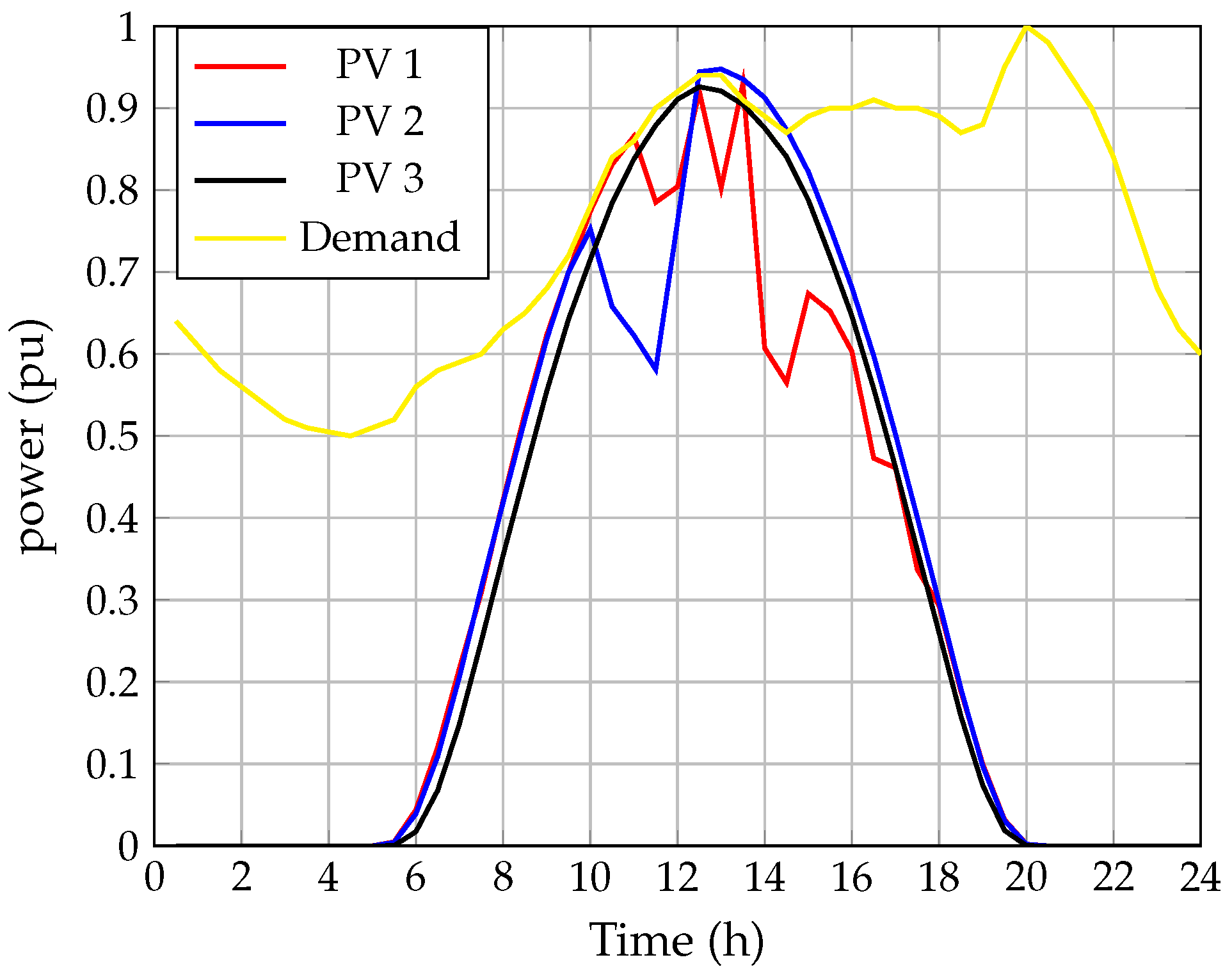
Numerical validations and scenarios are performed to validate the robust convex model’s performance in a modified 21-bus test system.

1.5. Document Organization

The structure of this contribution is the following: Section 2 presents the general formulation of the OPF problem for bipolar DC networks with unbalanced loads using the current injection method. This optimization model’s main characteristics are discussed, specifically the fact that it is nonlinear and non-convex. Section 3 presents the proposed convex approximation based on the linear approximation of the hyperbolic relation between voltages and powers in the constant power consumptions. In addition, a linear relaxation is applied for these relations in the PV generation sources. Section 4 describes the main characteristics of the test feeder, which is a medium voltage network composed of 21 nodes and 20 lines (radial configuration) operated with ±1 kV in terminals of the substation bus. This section also reveals the main numerical results of the proposed recursive convex approximation considering uncertainties in the generation output of the PV plants. Finally, Section 5 describes the main concluding remarks derived from this study and some possible future works.

2. Multiperiod OPF Formulation

The OPF model for bipolar DC networks considers multiple periods of analysis regarding generation and demand, and can be formulated as a nonlinear programming model from the family of non-convex optimization problems. The main idea in the multiperiod OPF problem is to minimize the total grid energy losses for an operation period of analysis (typically 24 h). This optimization is subject to the typical power flow constraints and device capabilities.

2.1. Mathematical Formulation

The complete NLP formulation of the multiperiod OPF problem for bipolar DC networks is described below.

Objective function:

$$\begin{array}{cc}\hfill & min{E}_{\mathrm{loss}}={\displaystyle \sum _{h\in \mathcal{H}}}{\displaystyle \sum _{r\in \mathcal{P}}}{\displaystyle \sum _{j\in \mathcal{N}}}{V}_{jh}^r\left({\displaystyle \sum _{s\in \mathcal{P}}}{\displaystyle \sum _{k\in \mathcal{N}}}{G_{jk}}^{rs}{V}_{kh}^s\right){\Delta }_h,\hfill \end{array}$$

(1)

Subject to:

$$\begin{array}{cc}\hfill & I_{g,kh}^p+I_{dg,kh}^p-I_{d,kh}^p-I_{d,kh}^{p-n}={\displaystyle \sum _{r\in \mathcal{P}}}{\displaystyle \sum _{j\in \mathcal{N}}}{G}_{jk}^{pr}{V}_k^r,\left\{\forall k\in \mathcal{N},\forall h\in \mathcal{H}\right\}\hfill \end{array}$$

(2)

$$\begin{array}{cc}\hfill & I_{g,kh}^o+I_{dg,kh}^o-I_{d,kh}^o-I_{d,kh}^{\mathrm{gr}}={\displaystyle \sum _{r\in \mathcal{P}}}{\displaystyle \sum _{j\in \mathcal{N}}}{G}_{jk}^{or}{V}_k^r,\left\{\forall k\in \mathcal{N},\forall h\in \mathcal{H}\right\}\hfill \end{array}$$

(3)

$$\begin{array}{cc}\hfill & I_{g,kh}^n+I_{dg,kh}^n-I_{d,kh}^n+I_{d,kh}^{p-n}={\displaystyle \sum _{r\in \mathcal{P}}}{\displaystyle \sum _{j\in \mathcal{N}}}{G}_{jk}^{nr}{V}_k^r,\left\{\forall k\in \mathcal{N},\forall h\in \mathcal{H}\right\}\hfill \end{array}$$

(4)

$$\begin{array}{cc}\hfill & I_{d,kh}^p=\frac{P_{d,kh}^p}{V_{kh}^p-V_{kh}^o},\left\{\forall k\in \mathcal{N},\forall h\in \mathcal{H}\right\}\hfill \end{array}$$

(5)

$$\begin{array}{cc}\hfill & I_{d,kh}^n=\frac{P_{d,kh}^n}{V_{kh}^n-V_{kh}^o},\left\{\forall k\in \mathcal{N},\forall h\in \mathcal{H}\right\}\hfill \end{array}$$

(6)

$$\begin{array}{cc}\hfill & I_{d,kh}^o=\frac{P_{d,kh}^p}{V_{kh}^o-V_{kh}^p}+\frac{P_{d,kh}^n}{V_k^o-V_k^n},\left\{\forall k\in \mathcal{N},\forall h\in \mathcal{H}\right\}\hfill \end{array}$$

(7)

$$\begin{array}{cc}\hfill & I_{d,khh}^{p-n}=\frac{P_{d,kh}^{p-n}}{V_{kh}^p-V_{kh}^n},\left\{\forall k\in \mathcal{N},\forall h\in \mathcal{H}\right\}\hfill \end{array}$$

(8)

$$\begin{array}{cc}\hfill & I_{dg,kh}^p=\frac{P_{dg,kh}^p}{V_{kh}^p-V_{kh}^o},\left\{\forall k\in \mathcal{N},\forall h\in \mathcal{H}\right\}\hfill \end{array}$$

(9)

$$\begin{array}{cc}\hfill & I_{dg,kh}^n=\frac{P_{dg,kh}^n}{V_{kh}^n-V_{kh}^o},\left\{\forall k\in \mathcal{N},\forall h\in \mathcal{H}\right\}\hfill \end{array}$$

(10)

$$\begin{array}{cc}\hfill & I_{dg,kh}^o=\frac{P_{dg,kh}^p}{V_{kh}^o-V_{kh}^p}+\frac{P_{dg,kh}^n}{V_{kh}^o-V_{kh}^n},\left\{\forall k\in \mathcal{N},\forall h\in \mathcal{H}\right\}\hfill \end{array}$$

(11)

$$\begin{array}{cc}\hfill & I_{g,kh}^{p,min}\le I_{g,kh}^p\le I_{g,kh}^{p,max},\left\{\forall k\in \mathcal{N},\forall h\in \mathcal{H}\right\}\hfill \end{array}$$

(12)

$$\begin{array}{cc}\hfill & I_{g,kh}^{o,min}\le I_{g,kh}^o\le I_{g,kh}^{o,max},\left\{\forall k\in \mathcal{N},\forall h\in \mathcal{H}\right\}\hfill \end{array}$$

(13)

$$\begin{array}{cc}\hfill & I_{g,kh}^{n,min}\le I_{g,kh}^n\le I_{g,kh}^{n,max},\left\{\forall k\in \mathcal{N},\forall h\in \mathcal{H}\right\}\hfill \end{array}$$

(14)

$$\begin{array}{cc}\hfill & P_{dg,kh}^{p,min}\le P_{dg,kh}^p\le P_{dg,kh}^{p,max},\left\{\forall k\in \mathcal{N},\forall h\in \mathcal{H}\right\}\hfill \end{array}$$

(15)

$$\begin{array}{cc}\hfill & P_{dg,kh}^{o,min}\le P_{dg,kh}^o\le P_{dg,kh}^{o,max},\left\{\forall k\in \mathcal{N},\forall h\in \mathcal{H}\right\}\hfill \end{array}$$

(16)

$$\begin{array}{cc}\hfill & P_{dg,kh}^{n,min}\le P_{dg,kh}^n\le P_{dg,kh}^{n,max},\left\{\forall k\in \mathcal{N},\forall h\in \mathcal{H}\right\}\hfill \end{array}$$

(17)

$$\begin{array}{cc}\hfill & V^{p,min}\le V_{kh}^p\le V^{p,max},\left\{\forall k\in \mathcal{N},\forall h\in \mathcal{H}\right\}\hfill \end{array}$$

(18)

$$\begin{array}{cc}\hfill & V^{n,min}\le V_{kh}^n\le V^{n,max},\left\{\forall k\in \mathcal{N},\forall h\in \mathcal{H}\right\}\hfill \end{array}$$

(19)

$$\begin{array}{cc}\hfill & \left[\begin{array}{c}{V}_{jh}^p\\ V_{jh}^o\\ V_{jh}^n\end{array}\right]=\left[\begin{array}{c}1\\ 0\\ -1\end{array}\right]V_{\mathrm{nom}},\left\{j=\mathrm{slack},\forall h\in \mathcal{H}.\right\}\hfill \end{array}$$

(20)

where $E_{\mathrm{loss}}$ represents the objective function value associated with the expected energy losses caused by the resistive effects in all the branches of the bipolar DC network for the analysis period; $V_{jh}^r$ is the voltage at node j contained in the set of nodes $\mathcal{N}$ at the period h (defined in the set of periods $\mathcal{H}$), for the pole r (contained at the set of poles $\mathcal{P}$); $V_{kh}^s$ represents the voltage value at node k in the period h for the pole s; ${G_{jk}}^{rs}$ means the conductance value that associates nodes j and k and poles r and s. $I_{g,kh}^p$, $I_{g,kh}^o$, and $I_{g,kh}^n$ represents the current injections in the slack source (node k) at each period for the positive, neutral, and negative poles, respectively; $I_{dg,kh}^p$, $I_{dg,kh}^o$, and $I_{dg,kh}^n$ have the same interpretation in case of the connection of dispersed generation source at node k. $I_{d,kh}^p$, $I_{d,kh}^o$, and $I_{d,kh}^n$ are the monopolar demanded currents at node k at time h for each one of the poles, respectively. $I_{d,kh}^{p-n}$ represents the bipolar demanded current by a load interconnected between the positive and negative poles. $I_{d,kh}^{\mathrm{gr}}$ represents the current drained to the earth in the neutral pole at node k at each time h when it is solidly grounded. $P_{d,kh}^p$ and $P_{d,kh}^n$ are the monopolar constant power consumptions at node k in period h connected between the neutral pole and the positive and negative ones, respectively. $V_{kh}^p$, $V_{kh}^o$, and $V_{kh}^n$ correspond to the voltage values at node k in the period h for the positive, neutral, and negative poles, respectively. $P_{dg,kh}^p$ and $P_{dg,kh}^n$ are the power injections by dispersed sources connected in positive and negative poles of node k in period h. $I_{g,kh}^{p,min}$, $I_{g,kh}^{o,min}$, and $I_{g,kh}^{n,min}$ are the minimum allowed bounds for the current injection in the slack source in positive, neutral and negative poles for node k in each period h; and $I_{g,kh}^{p,max}$, $I_{g,kh}^{o,max}$, and $I_{g,kh}^{n,max}$ are the upper current limits for the current injection in the slack source at each pole and time, respectively. $P_{dg,kh}^{o,min}$, $P_{dg,kh}^{p,min}$, and $P_{dg,kh}^{n,min}$ represent the minimum power injection bounds allowed for the dispersed source connected at node k for each pole in the period h, respectively. $P_{dg,kh}^{o,max}$, $P_{dg,kh}^{p,max}$, and $P_{dg,kh}^{n,max}$ are the maximum power injections allowed for the dispersed sources at each node, pole, and period, respectively. $V^{p,min}$ and $V^{n,min}$ are the minimum voltage regulation limits for voltages at each node and time for the positive and negative poles. In contrast, $V^{p,max}$ and $V^{n,max}$ are their corresponding upper regulation bounds, respectively. $V_{\mathrm{nom}}$ is the nominal voltage magnitude applied to the positive and negative poles.

2.2. Model Interpretation and Complexity

The interpretation of the NLP model (1)–(20) that represents the multiperiod OPF problem for bipolar asymmetry distribution networks is the following: Equation (1) represents the objective function of minimization which is associated with the energy losses of the network. Equations (2)–(4) represent the current equilibrium at each node of the network, which is obtained through the application of Kirchhoff’s first law at each one using the nodal voltage method. Equations (5)–(8) define the hyperbolic relation between power and voltages in all the demand nodes, and Equations (9)–(11) determine the hyperbolic relation between voltage and currents in the dispersed generation sources. Box-type constraints (12)–(14) define the solution space limits for the current injections in the slack source at each pole for each period of analysis. Box-type constraints (15)–(17) determine the solution space bounds for the dispersed generators integrated into the bipolar DC network. Box-type constraints (18) and (19) are the lower and upper bounds admissible for the voltage at each node and period, i.e., these are the classical voltage regulation constraints extended to bipolar DC configurations. Finally, Equation (20) defines the voltage output assigned in the terminals of the substation bus.

Even if the problem under investigation is part of the nonlinear programming models, the solution can be addressed via derivative-based optimization methods. It presents many variables that depend on the size of the test feeder under analysis. This number of variables is directly related to the complexity of the solution.

Table 1. Classification of the number of variables and equations for the optimization model (1)–(20).

Model Variables
Variable	Number	Variable	Number
Objective function	1	Voltages	$npt$
Currents	$\left(3p+2\right)nt$	Powers	$npt$
Total variables $\left(5p+2\right)nt+1$
Model equalities and inequalities
Equalities	$\left(3p+1\right)nt+pt+1$	Inequalities	$2\left(p+1\right)nt$
Total eq. and ineq. $\left(5p+3\right)nt+pt+1$

presents the detailed classification of the variables and equations that compose the optimization model. Note that this classification considers that the number of nodes is n, the number of poles is p, and the number of periods is t.

The main characteristic of the optimization problem is that from the total number of equalities and inequalities in the optimization model, only $\left(2p+1\right)nt$ are non-convex. These are related to the hyperbolic constraints regarding voltages and powers in the constant power terminals (demand and generation nodes), implying that these equations are convexified. Hence, the NLP model that represents the multiperiod optimal power flow problem for renewable generation can be optimally solved using the convex tool via recursive programming.

3. Approximated Recursive Quadratic Convex Model Formulation and Its Iterative Implementation

This section presents the proposed recursive quadratic approximation for solving the multiperiod OPF problem for bipolar DC networks with renewable generation sources. First, the model characterization is presented; second, the proposed convexification methodology and recursive solution approach are illustrated; and third, the robust optimization procedure is presented.

3.1. Characterization and Properties of the Optimization Model

In the NLP model (1)–(20), the following features can be observed:

i.

The objective function is a nonlinear quadratic function associated with multiple products between voltages. However, this is a convex function since the conductance matrix of the network is positive semidefinite [6]. Note that the objective function (1) can be rewritten as presented below.

$$\begin{array}{c}\hfill min{E}_{\mathrm{loss}}={\displaystyle \sum _{h\in \mathcal{H}}}{\left(V_h^{pon}\right)}^{\top }{G}_{pon}{V}_h^{pon}{\Delta }_h,\end{array}$$

(21)

which provides evidence that if $G_{pon}⪰0$, then the objective function is a sum of convex quadratic functions, i.e., a convex function. Note that $V_h^{pon}$ is a vector that contains all the nodal voltages ordered per pole and node, respectively.

ii.

The set of equality constraints (2)–(4), and (20) is part of the affine constraints, i.e., convex planes; in addition, box-type constraints (12)–(19) are linear inequality constraints that make part of a convex solution space.

iii.

The set of equality constraints (2)–(4), and (20) is part of the affine constraints, i.e., convex planes; in addition, box-type constraints (12)–(19) are linear inequality constraints that make part of a convex solution space.

iv

The set of equality constraints (5)–(11) represents the nonlinear non-convex set of equations for the problem under investigation, since these are hyperbolic constraints, which implies that to reach a convex equivalent optimization model, these must be convexified using linear or conic approximations.

In this study, we propose two linear approximations to obtain a convex approximated model for the multiperiod OPF problem defined in (1)–(20). These approximations are presented in the next section.

3.2. Convexification of the Hyperbolic Constraints

The following relaxations are proposed to obtain equivalent convex relaxations regarding the hyperbolic constraints that relate powers and voltages in constant power terminals and dispersed generators.

3.2.1. Proposed Convex Relaxation for Constant Power Loads

To reach a linear approximation (convex) of the hyperbolic constraint that associates voltages and power in constant load terminals, let us define an auxiliary function of the variables x, y, and the constant parameter w, as presented below [18,19].

$$\begin{array}{c}\hfill f\left(x,y\right)=\frac{w}{x-y},\end{array}$$

(22)

This function can be approximated in its linear form using Taylor’s series expansion, which corresponds to a linearization for a function of two continuous variables, which is defined below [19]:

$$\begin{array}{c}\hfill f\left(x,y\right)\approx f\left(x_0,y_0\right)+f_x\left(x_0,y_0\right)\left(x-x_0\right)+f_y\left(x_0,y_0\right)\left(y-y_0\right),\end{array}$$

(23)

where the point $\left(x_0,y_0\right)$ corresponds to the linearization point.

Now, if the linear approximation (23) is applied to the nonlinear function (22), then the linear approximation for this function is reached

$$\begin{array}{c}\hfill f\left(w,y\right)=\frac{2w}{x_0-y_0}-\frac{x-y}{{\left(x_0-y_0\right)}^2}w.\end{array}$$

(24)

Note that with the linear approximation (24), the demanded currents in the constant power terminals defined in (5)–(8) can be approximated by selecting $\left(x_0,y_0\right)$ as the initial voltage values for each pair of poles. ($V_k^{p,0}$, $V_k^{o,0}$. Further, $V_k^{n,0}$ are the initial values of the voltage profiles at note k for the positive, neutral, and negative poles, which can be defined initially equal to the voltage profile in the slack source as presented in Equation (20), and w is defined as the constant power load which can be monopolar or bipolar.) These equations are redefined linearly from (25) to (28).

$$\begin{array}{c}\hfill I_{d,kh}^{p,0}=P_{d,kh}^p\left(\frac{2}{V_{kh}^{p,0}-V_{kh}^{o,0}}-\frac{\left(V_{kh}^p-V_{kh}^o\right)}{{\left(V_{kh}^{p,0}-V_{kh}^{o,0}\right)}^2}\right)\left\{\forall k\in \mathcal{N},\forall h\in \mathcal{H}\right\}\end{array}$$

(25)

$$\begin{array}{c}\hfill I_{d,kh}^{n,0}=P_{d,kh}^n\left(\frac{2}{V_{kh}^{n,0}-V_{kh}^{o,0}}-\frac{V_{kh}^n-V_{kh}^o}{{\left(V_{kh}^{n,0}-V_{kh}^{o,0}\right)}^2}\right),\left\{\forall k\in \mathcal{N},\forall h\in \mathcal{H}\right\}\end{array}$$

(26)

$$\begin{array}{c}\hfill I_{d,kh}^{o,0}=\left[\begin{array}{c}{P}_{d,kh}^p\left(\frac{2}{V_{kh}^{o,0}-V_{kh}^{p,0}}-\frac{V_{kh}^o-V_{kh}^p}{{\left(V_{kh}^{o,0}-V_{kh}^{p,0}\right)}^2}\right)+\\ P_{d,kh}^n\left(\frac{2}{V_{kh}^{o,0}-V_{kh}^{n,0}}-\frac{V_{kh}^o-V_{kh}^n}{{\left(V_{kh}^{o,0}-V_{kh}^{n,0}\right)}^2}\right)\end{array}\right],\left\{\forall k\in \mathcal{N},\forall h\in \mathcal{H}\right\}\end{array}$$

(27)

$$\begin{array}{c}\hfill I_{d,kh}^{p-n,0}=P_{d,kh}^{p-n}\left(\frac{2}{V_{kh}^{p,0}-V_{kh}^{n,0}}-\frac{V_{kh}^p-V_{kh}^n}{{\left(V_{kh}^{p,0}-V_{kh}^{n,0}\right)}^2}\right).\left\{\forall k\in \mathcal{N},\forall h\in \mathcal{H}\right\}\end{array}$$

(28)

Note that $I_{d,kh}^{p,0}$, $I_{d,kh}^{o,0}$, $I_{d,kh}^{n,0}$ defines the linearized absorbed currents in the positive, neutral and negative poles in monopolar loads. $I_{d,kh}^{p-n,0}$ is the linearized absorbed current produced by a bipolar constant power load between positive and negative poles.

3.2.2. Proposed Convex Approximation for Nodes with Dispersed Generation Sources

To obtain a linear equivalent function of the hyperbolic relation between voltage and powers in dispersed generation plants, we consider a linear approximation proposed by the authors of [20], for monopolar DC networks with constant power loads.

$$\begin{array}{c}\hfill g\left(x,y,z\right)=\frac{z}{x-y},\end{array}$$

(29)

where we can consider that the numerator has strong variations in comparison with the denominator; in other words, the values of the variables x and y are near the operative point $\left(x_0,y_0\right)$. This means that ${\Delta }_{xy}\approx 0$, while the operative point of the power generator can present high oscillations. With this consideration, Equation (29) can be linearized as follows:

$$\begin{array}{c}\hfill g\left(x,y,z\right)\approx \frac{z}{x_0-y_0+{\Delta }_{xy}}\approx \frac{z}{x_0-y_0}.\end{array}$$

(30)

Now, considering the approximation presented in (30), it is possible to obtain a linear equivalent for the current injections with the dispersed sources in Equations (9)–(11), by defining the new variable z as the power injections of the dispersed sources, as presented below.

$$\begin{array}{c}\hfill I_{dg,kh}^p=\frac{P_{dg,kh}^p}{V_{kh}^{p,0}-V_{kh}^{o,0}},\left\{\forall k\in \mathcal{N},\forall h\in \mathcal{H}\right\}\end{array}$$

(31)

$$\begin{array}{c}\hfill I_{dg,kh}^n=\frac{P_{dg,kh}^n}{V_{kh}^{n,0}-V_{kh}^{o,0}},\left\{\forall k\in \mathcal{N},\forall h\in \mathcal{H}\right\}\end{array}$$

(32)

$$\begin{array}{c}\hfill I_{dg,kh}^o=\frac{P_{dg,kh}^p}{V_{kh}^{o,0}-V_{kh}^{p,0}}+\frac{P_{dg,kh}^n}{V_{kh}^{o,0}-V_{kh}^{n,0}}.\left\{\forall k\in \mathcal{N},\forall h\in \mathcal{H}\right\}\end{array}$$

(33)

Remark 1.

Note that the linear approximation of the demanded load currents via Taylor’s series expansion and the equivalent linear approximations for the dispersed generation sources allows transforming the original multiperiod nonlinear non-convex OPF problem into a convex approximation for bipolar DC networks with multiple constant power loads.

3.2.3. Recursive Quadratic Convex Approximation

If the linear approximations (25)–(28) for the constant power loads and the linear approximations (31)–(33) are analyzed, then it can be observed that these depend on the linearization point $\left(V_{kh}^{p,0},V_{kh}^{o,0},V_{kh}^{n,0}\right)$. This implies that an error between the exact model and these approximations is expected. However, as recommended by the authors of [20], this error can be minimized by introducing a recursive solution procedure, which is referred to in this study as the recursive quadratic convex approximation (RQCA). To obtain the RQCA, an iterative counter t is introduced to replace the initial value of the variables marked with a superscript 0. The complete RQCA model is defined below.

Obj. fun.:

$$\begin{array}{cc}\hfill & min{E}_{\mathrm{loss}}={\displaystyle \sum _{h\in \mathcal{H}}}{\displaystyle \sum _{r\in \mathcal{P}}}{\displaystyle \sum _{j\in \mathcal{N}}}{V}_{jh}^{r,t+1}\left({\displaystyle \sum _{s\in \mathcal{P}}}{\displaystyle \sum _{k\in \mathcal{N}}}{G_{jk}}^{rs}{V}_{kh}^{s,t+1}\right){\Delta }_h,\hfill \end{array}$$

(34)

S.t:

$$\begin{array}{cc}\hfill & I_{g,kh}^{p,t+1}+I_{dg,kh}^{p,t}-I_{d,kh}^{p,t+1}-I_{d,kh}^{p-n,t+1}={\displaystyle \sum _{r\in \mathcal{P}}}{\displaystyle \sum _{j\in \mathcal{N}}}{G}_{jk}^{pr}{V}_k^{r,t+1},\left\{\forall k\in \mathcal{N},\forall h\in \mathcal{H}\right\}\hfill \end{array}$$

(35)

$$\begin{array}{cc}\hfill & I_{g,kh}^{o,t+1}+I_{dg,kh}^{o,t}-I_{d,kh}^{o,t+1}-I_{d,kh}^{\mathrm{gr}}={\displaystyle \sum _{r\in \mathcal{P}}}{\displaystyle \sum _{j\in \mathcal{N}}}{G}_{jk}^{or}{V}_k^{r,t+1},\left\{\forall k\in \mathcal{N},\forall h\in \mathcal{H}\right\}\hfill \end{array}$$

(36)

$$\begin{array}{cc}\hfill & I_{g,kh}^{n,t+1}+I_{dg,kh}^{n,t}-I_{d,kh}^{n,t+1}+I_{d,kh}^{p-n,t+1}={\displaystyle \sum _{r\in \mathcal{P}}}{\displaystyle \sum _{j\in \mathcal{N}}}{G}_{jk}^{nr}{V}_k^{r,t+1},\left\{\forall k\in \mathcal{N},\forall h\in \mathcal{H}\right\}\hfill \end{array}$$

(37)

$$\begin{array}{cc}\hfill & I_{d,kh}^{p,t+1}=P_{d,kh}^p\left(\frac{2}{V_{kh}^{p,t}-V_{kh}^{o,t}}-\frac{\left(V_{kh}^{p,t+1}-V_{kh}^{o,t+1}\right)}{{\left(V_{kh}^{p,t}-V_{kh}^{o,t}\right)}^2}\right)\left\{\forall k\in \mathcal{N},\forall h\in \mathcal{H}\right\}\hfill \end{array}$$

(38)

$$\begin{array}{cc}\hfill & I_{d,kh}^{n,t+1}=P_{d,kh}^n\left(\frac{2}{V_{kh}^{n,t}-V_{kh}^{o,t}}-\frac{V_{kh}^{n,t+1}-V_{kh}^{o,t+1}}{{\left(V_{kh}^{n,t}-V_{kh}^{o,t}\right)}^2}\right),\left\{\forall k\in \mathcal{N},\forall h\in \mathcal{H}\right\}\hfill \end{array}$$

(39)

$$\begin{array}{cc}\hfill & I_{d,kh}^{o,t+1}=\left[\begin{array}{c}{P}_{d,kh}^p\left(\frac{2}{V_{kh}^{o,t}-V_{kh}^{p,t}}-\frac{V_{kh}^{o,t+1}-V_{kh}^{p,t+1}}{{\left(V_{kh}^{o,t}-V_{kh}^{p,t}\right)}^2}\right)+\\ P_{d,kh}^n\left(\frac{2}{V_{kh}^{o,t}-V_{kh}^{n,t}}-\frac{V_{kh}^{o,t+1}-V_{kh}^{n,t+1}}{{\left(V_{kh}^{o,t}-V_{kh}^{n,t}\right)}^2}\right)\end{array}\right],\left\{\forall k\in \mathcal{N},\forall h\in \mathcal{H}\right\}\hfill \end{array}$$

(40)

$$\begin{array}{cc}\hfill & I_{d,kh}^{p-n,t+1}=P_{d,kh}^{p-n}\left(\frac{2}{V_{kh}^{p,t}-V_{kh}^{n,t}}-\frac{V_{kh}^{p,t+1}-V_{kh}^{n,t+1}}{{\left(V_{kh}^{p,t}-V_{kh}^{n,t}\right)}^2}\right),\left\{\forall k\in \mathcal{N},\forall h\in \mathcal{H}\right\}\hfill \end{array}$$

(41)

$$\begin{array}{cc}\hfill & I_{dg,kh}^{p,t}=\frac{P_{dg,kh}^p}{V_{kh}^{p,t}-V_{kh}^{o,t}},\left\{\forall k\in \mathcal{N},\forall h\in \mathcal{H}\right\}\hfill \end{array}$$

(42)

$$\begin{array}{cc}\hfill & I_{dg,kh}^{n,t}=\frac{P_{dg,kh}^n}{V_{kh}^{n,t}-V_{kh}^{o,t}},\left\{\forall k\in \mathcal{N},\forall h\in \mathcal{H}\right\}\hfill \end{array}$$

(43)

$$\begin{array}{cc}\hfill & I_{dg,kh}^{o,t}=\frac{P_{dg,kh}^p}{V_{kh}^{o,t}-V_{kh}^{p,t}}+\frac{P_{dg,kh}^n}{V_{kh}^{o,t}-V_{kh}^{n,t}}.\left\{\forall k\in \mathcal{N},\forall h\in \mathcal{H}\right\}\hfill \end{array}$$

(44)

$$\begin{array}{cc}\hfill & I_{g,kh}^{p,min}\le I_{g,kh}^{p,t+1}\le I_{g,kh}^{p,max},\left\{\forall k\in \mathcal{N},\forall h\in \mathcal{H}\right\}\hfill \end{array}$$

(45)

$$\begin{array}{cc}\hfill & I_{g,kh}^{o,min}\le I_{g,kh}^{o,t+1}\le I_{g,kh}^{o,max},\left\{\forall k\in \mathcal{N},\forall h\in \mathcal{H}\right\}\hfill \end{array}$$

(46)

$$\begin{array}{cc}\hfill & I_{g,kh}^{n,min}\le I_{g,kh}^{n,t+1}\le I_{g,kh}^{n,max},\left\{\forall k\in \mathcal{N},\forall h\in \mathcal{H}\right\}\hfill \end{array}$$

(47)

$$\begin{array}{cc}\hfill & P_{dg,kh}^{p,min}\le P_{dg,kh}^p\le P_{dg,kh}^{p,max},\left\{\forall k\in \mathcal{N},\forall h\in \mathcal{H}\right\}\hfill \end{array}$$

(48)

$$\begin{array}{cc}\hfill & P_{dg,kh}^{o,min}\le P_{dg,kh}^o\le P_{dg,kh}^{o,max},\left\{\forall k\in \mathcal{N},\forall h\in \mathcal{H}\right\}\hfill \end{array}$$

(49)

$$\begin{array}{cc}\hfill & P_{dg,kh}^{n,min}\le P_{dg,kh}^n\le P_{dg,kh}^{n,max},\left\{\forall k\in \mathcal{N},\forall h\in \mathcal{H}\right\}\hfill \end{array}$$

(50)

$$\begin{array}{cc}\hfill & V^{p,min}\le V_{kh}^{p,t+1}\le V^{p,max},\left\{\forall k\in \mathcal{N},\forall h\in \mathcal{H}\right\}\hfill \end{array}$$

(51)

$$\begin{array}{cc}\hfill & V^{n,min}\le V_{kh}^{n,t+1}\le V^{n,max},\left\{\forall k\in \mathcal{N},\forall h\in \mathcal{H}\right\}\hfill \end{array}$$

(52)

$$\begin{array}{cc}\hfill & \left[\begin{array}{c}{V}_{jh}^{p,t+1}\\ V_{jh}^{o,t+1}\\ V_{jh}^{n,t+1}\end{array}\right]=\left[\begin{array}{c}1\\ 0\\ -1\end{array}\right]V_{\mathrm{nom}},\left\{j=\mathrm{slack},\forall h\in \mathcal{H}.\right\}\hfill \end{array}$$

(53)

Remark 2.

The optimization model (34)–(53) is a convex approximated model for the multiperiod OPF problem in bipolar DC networks for each $t+1$, assuming that the values in t are perfectly known. In addition, it is recursively solved until the convergence criterion between two consecutive iterations is met, as follows:

$$\begin{array}{c}\hfill {\displaystyle \underset{\left\{k\in \mathcal{N},h\in \mathcal{H},r\in \mathcal{P}\right\}}{max}}\left|\left|V_{kh}^{p,t+1}\right|-\left|V_{kh}^{p,t}\right|\right|\le \epsilon ,\end{array}$$

(54)

where ε is defined as $1\times {10}^{-10}$.

3.3. Robust RQCA Model

The robust optimization determines the worst case for the problem to be optimized. For this purpose, it is necessary to use two sets of variables. The former set denotes decision variables (x) of the problem, and the latter set proposes uncertain variables (w). The objective of robust optimization lies in finding a solution to the decision variables in such a form that it minimizes the problem under worst-case cost, satisfying its set of constraints and, at the same time, allows uncertainty variables to take arbitrary values. In a general form, a problem of robust optimization can be written as follows [14]:

$$\begin{array}{c}\hfill \begin{array}{cc}\hfill \underset{x}{min}\underset{w}{max}& f(x,w),\hfill \\ \hfill \mathrm{subject}\mathrm{to}& g_1(x,w)=0\forall w\in \mathcal{W},\hfill \\ \hfill & g_2(x,w)\le 0\forall w\in \mathcal{W},\hfill \end{array}\end{array}$$

(55)

where $f(x,w)$ is the objective function that considers the uncertain variables, and $g_1(x,w)$ and $g_2(x,w)$ are the equality and inequalities constraint sets, respectively.

In order to introduce the uncertain variables in the proposed model, it is necessary to define the following variables

$$\begin{array}{c}\hfill {\theta }_{kh}^{p+}+{\theta }_{kh}^{p-}\le 1,\left\{\forall k\in \mathcal{N},\forall h\in \mathcal{H}\right\}\end{array}$$

(56)

$$\begin{array}{c}\hfill {\theta }_{kh}^{n+}+{\theta }_{kh}^{n-}\le 1,\left\{\forall k\in \mathcal{N},\forall h\in \mathcal{H}\right\}\end{array}$$

(57)

$$\begin{array}{c}\hfill P_{dg,kh}^p={\overline{P}}_{dg,kh}^p+{\widehat{P}}_{dg,kh}^p{\theta }_{kh}^{p+}-{\widehat{P}}_{dg,kh}^p{\theta }_{kh}^{p-},\left\{\forall k\in \mathcal{N},\forall h\in \mathcal{H}\right\}\end{array}$$

(58)

$$\begin{array}{c}\hfill P_{dg,kh}^n={\overline{P}}_{dg,kh}^n+{\widehat{P}}_{dg,kh}^n{\theta }_{kh}^{n+}-{\widehat{P}}_{dg,kh}^n{\theta }_{kh}^{n-},\left\{\forall k\in \mathcal{N},\forall h\in \mathcal{H}\right\}\end{array}$$

(59)

where $\theta$ is a binary variable used to denote the uncertainty set, ${\overline{P}}_{dg}$ is the power injection of the solar generator, and ${\widehat{P}}_{dg}$ is the power deviation of the solar generator from its nominal value.

From (58) and (59), we can note that $P_{dg,kh}^p$ and $P_{dg,kh}^n$ take values within the following interval

$$\begin{array}{c}\hfill P_{dg,kh}^p\in [{\overline{P}}_{dg,kh}^p-{\widehat{P}}_{dg,kh}^p,{\overline{P}}_{dg,kh}^p+{\widehat{P}}_{dg,kh}^p]\end{array}$$

(60)

$$\begin{array}{c}\hfill P_{dg,kh}^n\in [{\overline{P}}_{dg,kh}^n-{\widehat{P}}_{dg,kh}^n,{\overline{P}}_{dg,kh}^n+{\widehat{P}}_{dg,kh}^n]\end{array}$$

(61)

Finally, the proposed robust mode takes the following form

$$\underset{V}{min}\left(E_{\mathrm{loss}}max∥{\overline{P}}_{dg}^p∥+∥{\overline{P}}_{dg}^n∥\right)$$

(62)

subject to (34)–(40), (44)–(52), (56)–(59).

Algorithm 1 provides the flowchart of the proposed robust recursive quadratic convex model.

Algorithm 1: Robust Recursive Quadratic Convex Algorithm.

4. Test System and Results

This section presents the main characteristics of the bipolar DC distribution network and all the numerical validations. Note that the deterministic and robust optimization model will be evaluated for validation.

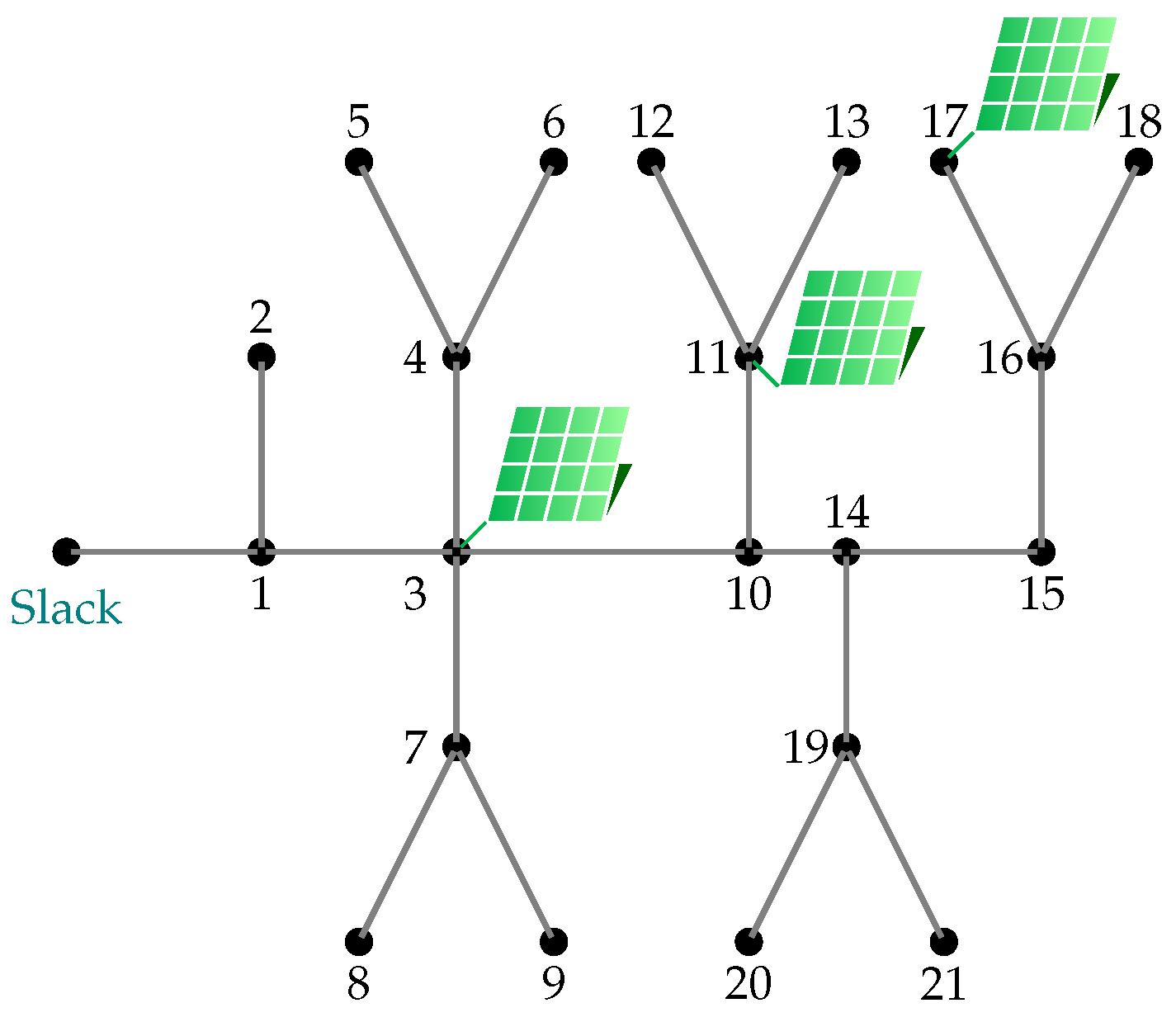
4.1. Bipolar DC 21-Bus System

The robust RQCA proposed is evaluated in the modified 21-bus bipolar DC system. This system is a modification of the proposed test system presented in [21] for a monopolar DC network. Figure 1 illustrates the modified 21-bus bipolar DC network with three PV generators. The slack node operates with a rated voltage of ±1 kV in the positive and negative poles with a neutral pole that is solidly grounded. This test system has a whole power consumption in the positive pole of 554 kW, while the negative pole is at 445 kW.

Table 2. Data information for the modified 21-bus bipolar DC system.

Node k	Node m	${\mathit{R}}_{\mathit{km}}$ (Ω)	${\mathit{P}}_{\mathit{d},2}^{\mathit{p}}$ (kW)	${\mathit{P}}_{\mathit{d},2}^{\mathit{n}}$ (kW)	${\mathit{P}}_{\mathit{d},2}^{\mathit{p}-\mathit{n}}$ (kW)
1	2	0.053	70	100	0
1	3	0.054	0	0	0
3	4	0.054	36	40	120
4	5	0.063	4	0	0
4	6	0.051	36	0	0
3	7	0.037	0	0	0
7	8	0.079	32	50	0
7	9	0.072	80	0	100
3	10	0.053	0	10	0
10	11	0.038	45	30	0
11	12	0.079	68	70	0
11	13	0.078	10	0	75
10	14	0.083	0	0	0
14	15	0.065	22	30	0
15	16	0.064	23	10	0
16	17	0.074	43	0	60
16	18	0.081	34	60	0
14	19	0.078	9	15	0
19	20	0.084	21	10	50
19	21	0.082	21	20	0

lists all the data information of the modified 21-bus bipolar DC system.

The PV systems of the modified 21-bus bipolar DC system are located at nodes 3, 11, and 17. Their available powers are depicted in Figure 2, and this information was taken from [22]. In addition, this figure shows the demand variation during 24 h.

Table 3. Location and capacity of the PV generators.

Label	Node	Pole	Capacity (kW)	Label	Node	Pole	Capacity (kW)
PV 1	3	p	300	PV 3	17	p	200
	3	n	100		17	n	300
PV 2	11	p	400

shows each PV system’s rated power in the positive and negative poles.

4.2. Numerical Validation and Analysis of Results

The robust RQCA model was assessed on a personal computer (Dell Inspiron 15 7000 Series (Intel Quad-Core i7-7700HQ), 2.80 GHz, 16 GB RAM with 64-bit Windows 10 Home Single Language) using the software MATLAB 2021a. Additionally, Yalmip toolbox [23] plus Gurobi solver [24] were used to solve the proposed model.

4.2.1. Deterministic Model

This part assesses the RQCA model (34)–(53) solution for solving the OPF problem in bipolar asymmetric DC networks considering multiple PV generators. Firstly, the proposed model is evaluated for nominal values of the bipolar DC network and compared with three metaheuristic optimization algorithms proposed in the specialized literature. The metaheuristics are the sine cosine algorithm (SCA) [25], the vortex search algorithm (VSA) [26], and the black hole optimizer (BHO) [27]. A convergence error of $\epsilon =1\times {10}^{-10}$ was considered for these metaheuristics. In addition, 1000 iterations, 10 individuals, and 100 consecutive repetitions were performed for each metaheuristic optimization algorithm. Secondly, the proposed model was analyzed for 24 h to determine the effect of the multiple PV generators in the bipolar DC network.

The results of the metaheuristic optimization algorithms and the proposed model are compared in

Table 4. Comparison of the models for solving the OPF problem ($P_{base}=100$ kW).

PV Capacity	Method	Min. (pu)	Mean (pu)	Max. (pu)	Std. Dev. (pu)	Average Time (s)
0%	SCA	0.9542368	0.9542368	0.9542368	$1.1\times {10}^{-15}$	4.6461
	VSA	0.9542368	0.9542368	0.9542368	$1.1\times {10}^{-16}$	4.1939
	BHO	0.9542368	0.9542368	0.9542368	$1.1\times {10}^{-16}$	9.2526
	RQCA	0.9542367	0.9542367	0.9542368	<$1\times {10}^{-16}$	6.0529
50%	SCA	0.3157859	0.3299539	0.3441219	$8.3\times {10}^{-3}$	4.5489
	VSA	0.3152253	0.3153301	0.3164762	$2.1\times {10}^{-4}$	5.2673
	BHO	0.3216582	0.3269265	0.3312492	$2.1\times {10}^{-1}$	9.1321
	RQCA	0.3152552	0.3152552	0.3152552	<$1\times {10}^{-16}$	5.8552
100%	SCA	0.2306334	0.2529280	0.2854381	$1.4\times {10}^{-2}$	4.3451
	VSA	0.2298536	0.2298567	0.2298805	$4.6\times {10}^{-6}$	5.0126
	BHO	0.2306558	0.2317489	0.2327831	$4.9\times {10}^{-4}$	9.1541
	RQCA	0.2298554	0.2298554	0.2298554	<$1\times {10}^{-16}$	6.1220

. This table shows the performance of the proposed model and metaheuristic optimization algorithms, considering that the PV generators are at 0, 50, and 100 % of their nominal capacity.

From Table 4 is possible to analyze that:

• The proposed RQCA reaches the global optimum for three levels of capacity of the PV generators with the solutions of $95.423$ kW, $31.525$ kW, and $22.985$ kW for 0%, 50%, and 100% of the capacity PV rating, respectively. The VSA algorithm shows numerical solutions similar to the proposed RQCA model. However, the proposed model always reaches the global optimum in each evaluation. This is because the proposed RQCA model is convex; hence, it finds the global optimum of the problem. By contrast, the VSA algorithm and other algorithms do not always reach the same solution, as these methods cannot guarantee a global solution to the problem.
• As the capacity level of the PVs increases, the solutions of the metaheuristic algorithms move away from the optimum solution. This is because these algorithms contain a random nature and simple evolution rules. In addition, the SCA and BHO algorithms present less sophisticated rules than the VSA algorithm, and for this reason, their performances are inferior to the VSA algorithm.

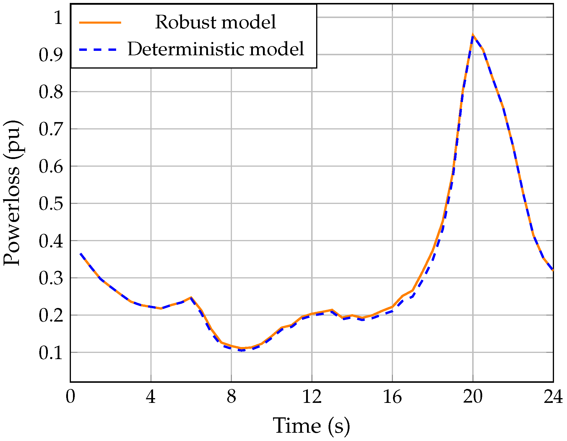
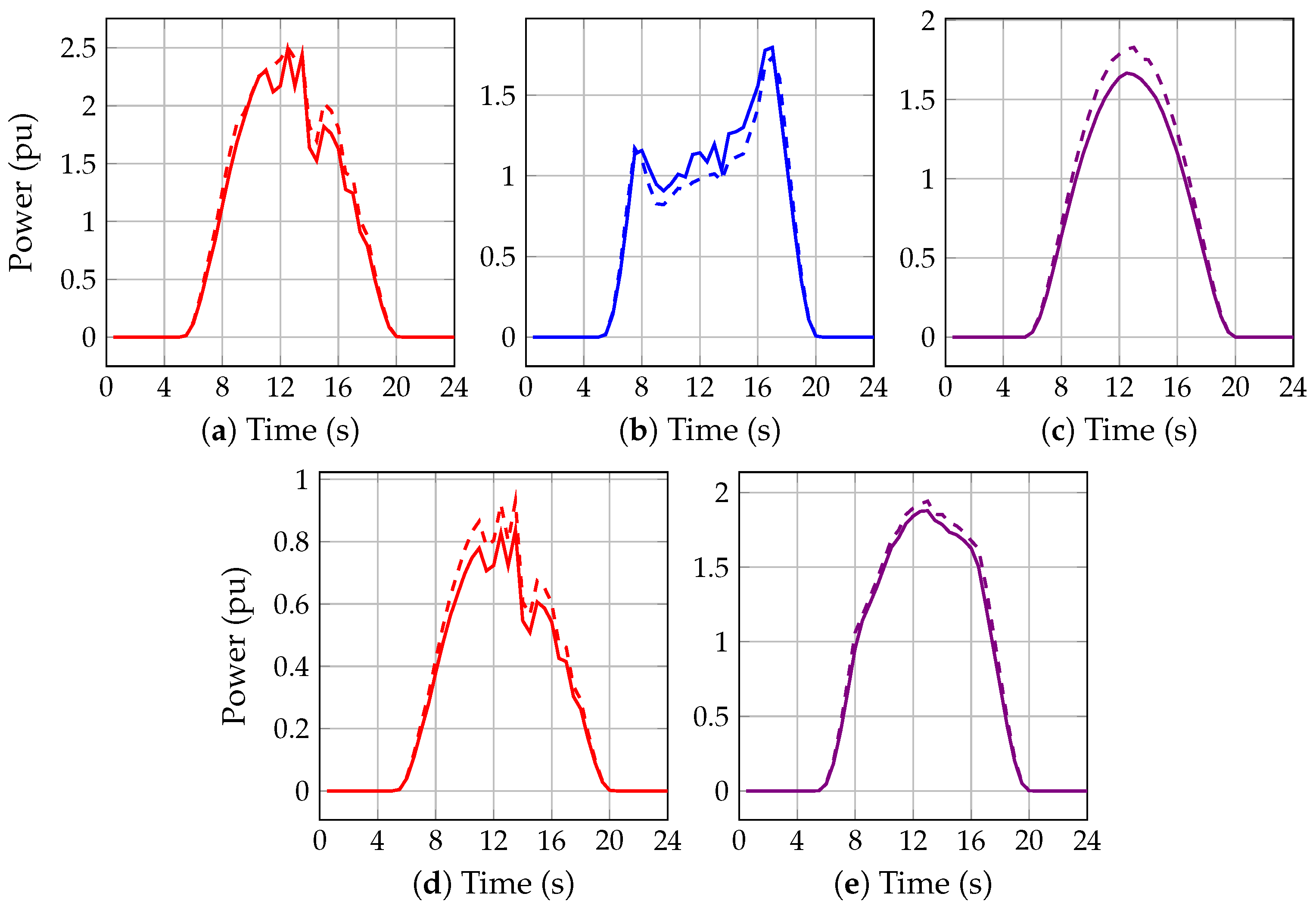
Figure 3 depicts the results of the proposed model for the optimal scheduling of PV generators in the modified 21-bus bipolar DC system. For this analysis and the following ones, only the results of the proposed model will be presented since, as seen in Table 4, the metaheuristic algorithms achieve lower results. Figure 3a illustrates the power losses of the bipolar DC grid at each hour. Figure 3b,c show the power delivered for the PV generators in the positive and negative poles, respectively.

Figure 3 shows that the power loss in the bipolar DC grid presents its highest value at 20:00 h; this occurs when the demand is highest, and there are no variables in the PV generators. Therefore, after 20:00 h, the slack node only satisfies the demand. The total power loss in the bipolar DC grid is 1513.401 kW. Analyzing Figure 3b, it can be noted that the PV generators connected to the positive pole deliver the whole available power to the bipolar DC grid between 00:00 h and 7:30 h as well as between 17:30 h and 24:00 h. At the same time, the PV generators connected to the negative pole generate the total available power from 00:00 to 8:00 h and from 16:30 h to 24:00 h (see Figure 3c). In contrast, when the PV generators do not deliver the total available power, the bipolar DC grid presents the least power losses. This is because the grid disposes of the necessary power to find the best point of operation. Further, observe in Figure 3b that the PV generator connected to node 11 (PV 2) is the generator that does not behave similarly to the available power.

4.2.2. Robust Model

This paper analyzes the performance of the proposed robust model (62) to compute the OPF problem in bipolar asymmetric DC networks with multiple PV systems. In addition, uncertainty in the available rated power of the PV systems $\pm 10\%$ is considered, as shown in Figure 4.

Figure 5 illustrates the power losses of the proposed robust RQCA model in the modified 21-bus bipolar DC system. Furthermore, this figure presents the power losses of the deterministic model in order to make a comparative analysis of the results.

In Figure 5, it can be seen that the behavior of the power losses of the robust model is similar to when uncertainties in PV generators are not considered. It is also to be expected that power losses increase considering the PV generator uncertainties, since the robust model works in the worst-case scenario. For this reason, in the hours when there is more significant uncertainty (period from 06:00 to 18:00), the power losses are higher. In this scenario, the total power loss in the bipolar DC grid is 1538.406 kW, increasing the power loss by 1.65% concerning the deterministic model.

Figure 6 shows a comparison between the power delivered by the PV generators when the robust model (solid line) and the deterministic model (dashed line) are implemented.

In Figure 5, the powers delivered by the PV generators for the robust model are lower than for the deterministic model. This behavior is expected since the robust model determines the worst case, selecting the configuration for the PV generators with the highest uncertainty. However, this trend is not seen in the PV generator connected to node 11 since it can deliver more energy in hours of more significant uncertainty. For this reason, there was no significant change in the power losses between models.

It is worth mentioning that the physical meaning of the power generation in Figure 3 and Figure 6 is that with these power values, the bipolar DC grid found its optimal operation point, which is minimal power loss. These powers permit maintaining the energy balance in each node of the bipolar DC grid.

5. Conclusions

In this work, a robust RQCA for scheduling optimal PV generators in bipolar asymmetric DC distribution grids was described. Initially, the proposed model relaxed the constraints that involve the hyperbolic relation between constant power terminals and voltage profiles. This relaxation was based on Taylor’s series expansion. Furthermore, the proposed model was resolved recursively to eliminate the errors introduced by relaxation. Numerical simulations were performed in a modified 21-bus test system to validate the robust convex model’s performance. These simulations were carried out in the MATLAB programming environment using Yalmip and Gurobi solver to evaluate the performance of the proposed model.

i.

In the proposed optimization approach, uncertainties in power available for the PV generators were considered. To solve this problem, the proposed methodology was transformed to a min–max problem, in which the problem solution is under worst-case cost, satisfying the set of constraints. This transformation becomes the proposed model in a robust model.

ii.

The proposed model was compared to three metaheuristic methods to show its effectiveness and validity, where it consistently achieved better solutions than the other methods.

iii.

The proposed solution methodology was evaluated in a scenario of 24 h using deterministic and robust models. The results show that, in the scenario of 24 h, the behavior of the power losses was similar between models. The results for the power losses in the proposed robust model were higher than the deterministic model. These results are expected since the robust mode works in the worst-case scenario.

Some future works that can be developed following this research are the following: (i) the inclusion in the proposed convex optimization method of the presence of battery energy storage systems in the bipolar DC grid; and (ii) the extension of the proposed optimization method via mixed-integer convex optimization to deal with the problem of the optimal placement and sizing of renewable energy resources in bipolar asymmetric distribution networks.

References

1. Mishra, S.; Das, D.; Paul, S. A comprehensive review on power distribution network reconfiguration. Energy Syst. 2016, 8, 227–284. [Google Scholar] [CrossRef]
2. Prakash, K.; Lallu, A.; Islam, F.; Mamun, K. Review of Power System Distribution Network Architecture. In Proceedings of the 2016 3rd Asia-Pacific World Congress on Computer Science and Engineering (APWC on CSE), Nadi, Fiji, 5–6 December 2016; IEEE: Piscataway, NJ, USA, 2016. [Google Scholar] [CrossRef]
3. Mousavizadeh, S.; Bolandi, T.G.; Alahyari, A.; Dadashzade, A.; Haghifam, M.R. A novel unbalanced power flow analysis in active AC-DC distribution networks considering PWM convertors and distributed generations. Int. J. Electr. Power Energy Syst. 2022, 138, 107938. [Google Scholar] [CrossRef]
4. Geng, Q.; Hu, Y.; He, J.; Zhou, Y.; Zhao, W.; Xu, X.; Wei, W. Optimal operation of AC–DC distribution network with multi park integrated energy subnetworks considering flexibility. IET Renew. Power Gener. 2020, 14, 1004–1019. [Google Scholar] [CrossRef]
5. Gao, S.; Liu, S.; Liu, Y.; Zhao, X.; Song, T.E. Flexible and Economic Dispatching of AC/DC Distribution Networks Considering Uncertainty of Wind Power. IEEE Access 2019, 7, 100051–100065. [Google Scholar] [CrossRef]
6. Garces, A. Uniqueness of the power flow solutions in low voltage direct current grids. Electr. Power Syst. Res. 2017, 151, 149–153. [Google Scholar] [CrossRef]
7. Montoya, O.D.; Serra, F.M.; Angelo, C.H.D. On the Efficiency in Electrical Networks with AC and DC Operation Technologies: A Comparative Study at the Distribution Stage. Electronics 2020, 9, 1352. [Google Scholar] [CrossRef]
8. Montoya, O.D.; Medina-Quesada, Á.; Hernández, J.C. Optimal Pole-Swapping in Bipolar DC Networks Using Discrete Metaheuristic Optimizers. Electronics 2022, 11, 2034. [Google Scholar] [CrossRef]
9. Noreña, L.F.G.; Rivera, O.D.G.; Toro, J.A.O.; Paja, C.A.R.; Cabal, M.A.R. Metaheuristic Optimization Methods for Optimal Power Flow Analysis in DC Distribution Networks. Trans. Energy Syst. Eng. Appl. 2020, 1, 13–31. [Google Scholar] [CrossRef]
10. Mackay, L.; Dimou, A.; Guarnotta, R.; Morales-Espania, G.; Ramirez-Elizondo, L.; Bauer, P. Optimal power flow in bipolar DC distribution grids with asymmetric loading. In Proceedings of the 2016 IEEE International Energy Conference (ENERGYCON), Piscataway, NJ, USA, 4–8 April 2016; IEEE: Piscataway, NJ, USA, 2016. [Google Scholar] [CrossRef]
11. Lee, J.O.; Kim, Y.S.; Jeon, J.H. Optimal power flow for bipolar DC microgrids. Int. J. Electr. Power Energy Syst. 2022, 142, 108375. [Google Scholar] [CrossRef]
12. Medina-Quesada, Á.; Montoya, O.D.; Hernández, J.C. Derivative-Free Power Flow Solution for Bipolar DC Networks with Multiple Constant Power Terminals. Sensors 2022, 22, 2914. [Google Scholar] [CrossRef] [PubMed]
13. Chew, B.S.H.; Xu, Y.; Wu, Q. Voltage Balancing for Bipolar DC Distribution Grids: A Power Flow Based Binary Integer Multi-Objective Optimization Approach. IEEE Trans. Power Syst. 2019, 34, 28–39. [Google Scholar] [CrossRef] [Green Version]
14. Löfberg, J. Automatic robust convex programming. Optim. Methods Softw. 2012, 27, 115–129. [Google Scholar] [CrossRef] [Green Version]
15. Mackay, L.; Guarnotta, R.; Dimou, A.; Morales-Espana, G.; Ramirez-Elizondo, L.; Bauer, P. Optimal power flow for unbalanced bipolar DC distribution grids. IEEE Access 2018, 6, 5199–5207. [Google Scholar] [CrossRef]
16. Lee, J.O.; Kim, Y.S.; Moon, S.I. Current injection power flow analysis and optimal generation dispatch for bipolar DC microgrids. IEEE Trans. Smart Grid 2020, 12, 1918–1928. [Google Scholar] [CrossRef]
17. Jat, C.K.; Dave, J.; Van Hertem, D.; Ergun, H. Unbalanced OPF Modelling for Mixed Monopolar and Bipolar HVDC Grid Configurations. arXiv 2022, arXiv:2211.06283. [Google Scholar]
18. Montoya, O.D.; Gil-González, W.; Hernández, J.C. Optimal Power Flow Solution for Bipolar DC Networks Using a Recursive Quadratic Approximation. Energies 2023, 16, 589. [Google Scholar] [CrossRef]
19. Kwok, Y.K. Applied Complex Variables for Scientists and Engineers; Cambridge University Press: Cambridge, UK, 2010. [Google Scholar]
20. Montoya, O.D.; Zishan, F.; Giral-Ramírez, D.A. Recursive Convex Model for Optimal Power Flow Solution in Monopolar DC Networks. Mathematics 2022, 10, 3649. [Google Scholar] [CrossRef]
21. Garces, A. On the Convergence of Newton’s Method in Power Flow Studies for DC Microgrids. IEEE Trans. Power Appar. Syst. 2018, 33, 5770–5777. [Google Scholar] [CrossRef] [Green Version]
22. Radiation data, S.S. Solar Training. Available online: http://www.soda-pro.com/ (accessed on 28 March 2022).
23. Löfberg, J. YALMIP: A Toolbox for Modeling and Optimization in MATLAB. In Proceedings of the 2004 IEEE International Conference on Robotics and Automation, New Orleans, LA, USA, 26 April–1 May 2004. [Google Scholar]
24. Gurobi Optimization, LLC. Gurobi Optimizer Reference Manual. 2022. Available online: http://www.gurobi.com (accessed on 5 January 2023).
25. Gabis, A.B.; Meraihi, Y.; Mirjalili, S.; Ramdane-Cherif, A. A comprehensive survey of sine cosine algorithm: Variants and applications. Artif. Intell. Rev. 2021, 54, 5469–5540. [Google Scholar] [CrossRef] [PubMed]
26. Doğan, B.; Ölmez, T. Vortex search algorithm for the analog active filter component selection problem. AEU-Int. J. Electron. Commun. 2015, 69, 1243–1253. [Google Scholar] [CrossRef]
27. Kumar, S.; Datta, D.; Singh, S.K. Black Hole Algorithm and Its Applications. In Studies in Computational Intelligence; Springer International Publishing: Berlin/Heidelberg, Germany, 2014; pp. 147–170. [Google Scholar] [CrossRef]
Figure 1. Single diagram of the modified 21-bus bipolar DC network.
Machines 11 00177 g001
Figure 2. Available power curve of the three PV generators and demand variation.
Machines 11 00177 g002
Figure 3. Optimal scheduling of PV generators: (a) power losses of the bipolar DC grid, (b) power delivered for the PV generators in the positive pole, and (c) power delivered for the PV generators in the negative pole.
Machines 11 00177 g003
Figure 4. Power available for the PV generators with Uncertainty ± 10 % : (a) PV generator connected to node 3, (b) PV generator connected to node 11, and (c) PV generator connected to node 17.
Machines 11 00177 g004
Figure 5. Comparison between the robust and deterministic model of the power losses of the bipolar DC grid.
Machines 11 00177 g005
Figure 6. The dispatched PV power for the robust model (solid line) and the deterministic model (dashed line): (a) PV generator connected to positive pole at node 3, (b) PV generator connected to positive pole at node 11, (c) PV generator connected to positive pole at node 17, (d) PV generator connected to negative pole at node 3, and (e) PV generator connected to negative pole at node 17.
Machines 11 00177 g006