Exponential Local Fisher Discriminant Analysis with Sparse Variables Selection: A Novel Fault Diagnosis Scheme for Industry Application

Abstract

Local Fisher discriminant analysis (LFDA) has been widely applied to dimensionality reduction and fault classification fields. However, it often suffers from small sample size (SSS) problem and incorporates all process variables without emphasizing the key faulty ones, thus leading to degraded fault diagnosis performance and poor model interpretability. To this end, this paper develops the sparse variables selection based exponential local Fisher discriminant analysis (SELFDA) model, which can overcome the two limitations of basic LFDA concurrently. First, the responsible faulty variables are identified automatically through the least absolute shrinkage and selection operator, and the current optimization problem are subsequently recast as an iterative convex optimization problem and solved by the minimization-maximization method. After that, the matrix exponential strategy is implemented on LFDA, it can essentially overcome the SSS problem by ensuring that the within-class scatter matrix is always full-rank, thus more practical in real industrial practices, and the margin between different categories is enlarged due to the distance diffusion mapping, which is benefit for the enhancement of classification accuracy. Finally, the Tennessee Eastman process and a real-world diesel working process are employed to validate the proposed SELFDA method, experimental results prove that the SELFDA framework is more excellent than the other approaches.

1. Introduction

Due to the gradually increasing requirements on system property, product quality as well as economic benefits, modern industrial processes have become even more complicated [1]. Hence, modern industrial processes urgently need advanced fault detection and isolation (FDI) techniques. Reviewing the existing FDI methods, there are two main subclasses: the data-based ones and the model-based ones. Specially, the data-based methods have been ever-accelerated recently with the continuously development of data collection and storage technologies, and received broad attention in both academy and industry domains [2,3,4,5]. Recently, lots of mature data-based approaches have been found applications in FDI field with great successes, which is also the focus of this paper.

Among all the data-based methods mentioned above, it is noteworthy that Fisher discriminant analysis (FDA) [6,7] and principal component analysis (PCA) [8,9] are the two most popular ones. In general, PCA and its extensions are an unsupervised feature extraction method and ignore the correlations among different faults. Hence, it is more suitable for fault detection rather than fault classification. In contrast, FDA belongs to supervised dimension reduction and feature extraction method, it selects a set of vectors that maximize the distance among classes while minimize the distance between classes simultaneously, have also becomes one of the research hotspots in classifying the detected process abnormalities nowadays [10].

Despite the fact that FDA is a popular fault classification model, it tends to show degraded performance if the samples in a class show multimodality. In response to this problem, a method named local Fisher discriminant analysis (LFDA) was originally presented in [11] for dimensionality reduction. LFDA aims to overcome the limitations of local preserving projection (LPP), which cannot select the most discriminative basis vectors to construct the subspace. Simultaneously, LFDA addresses the issue of unsatisfactory classification performance of traditional FDA when dealing with multi-modal problems. By combining locality-preserving projection and Fisher Discriminant Analysis, LFDA enhances the discriminative power of features. It achieves this by preserving similarity within the local structure of the data and optimizing global discriminability through the Fisher criterion. LFDA is particularly suitable for handling multi-modal data. Then, Yu applied this method to complex chemical process monitoring [12] and shown high sensitivity in diagnosing multiple faults. After that, the authors of [13] extended the LFDA to its multiway variation and performed much better in classifying faults as well as detecting abnormal operating conditions in fed-batch operation. Furthermore, the authors of [14] developed JFDA method to describe the process dataset from both the global and local view in a high-dimensional space and received satisfactory diagnosis performance in Tennessee Eastman (TE) process. Recently, Zhong et al. [15] proposed the sparse LFDA model, which can exploit the local data information from multiple dimensions and ease the problem of multimodality and nonlinearity. Ma et al. [16] presented the hierarchical strategy based on LFDA and canonical variable analysis (CVA) for hot strip mill process monitoring.

Nevertheless, the above LFDA-based methods typically assume that the relationships between samples have been correctly described. However, this assumption can be easily violated since the relations among the operating variables are also intricate. In such context, the variable selection strategy is necessary for feature filtering and better model interpretability, drawing great attention in both industry and academia. What is more, when the dimension of dataset is bigger than the number of samples (i.e., the small-sample-size (SSS) problem). Then the LFDA-based methods will confront with singular problem due to the irreversibility of the within-class scatter matrix. Given the reliability of LFDA in the field of fault diagnosis and classification, the following two problems maybe formidable challenges: One major challenge is how to implement proper improvements on LFDA to release the hypothesis that every sample of training data should be labeled accurately beforehand. Another challenge lies in the adverse effects on model classification performance that caused by singular data matrix.

To deal with the first predicament, an alternative way could be utilizing the useful information from labeled and unlabeled samples simultaneously [17,18], thus both the supervised information and intrinsic global structure are considered. Such methods are called the semi-supervised ones and they also have been applied to fault classification field. For example, ref. [18] proposed the semi-supervised form of the FDA (SFDA), which incorporated the supererogatory unlabeled samples when conducting the fault diagnosis model, showing better fault classification over FDA and PCA. Yan et al. presented the semi-supervised mixture discriminant analysis (SMDA) [19] to monitor batch processes and both the known and unknown faults have been diagnosed correctly. Recently, researchers combined the active learning with the semi-supervised EDA model and applied to process industries successfully [20], thus improving the applicability of the traditional EDA model in real industrial processes. However, the semi-supervised LFDA for fault classification has not been studied yet in existing literatures.

When encountering the likely and common SSS problem in practical scenarios, none of these approaches can be applied to that case directly since the within-class scatter matrix in question is singular, if an appropriate technique is utilized to solve up the SSS problem, then the model could be more broadly applicable. Fortunately, several modified methods have been provided in [21,22] to relieve the SSS problem to some extent. Nevertheless, the intrinsic limitation of FDA has not eliminated and the SFDA model could completely solve the SSS problem neither. Afterwards, Zhang et al. [23] proposed a novel advantageous FDA model from the matrix exponential perspective, which has settled the SSS problem thoroughly and show superior performance on various experiments. Soon after that, Adil et al. [24] applied the EDA model to fault diagnosis in industrial process with improved classification accuracy. Note that the authors of [25] also incorporated the exponential technique into LDE and showed better performance than the current discriminant analysis techniques in face recognition. More recently, Yu et al. [26] developed the exponential slow feature analysis (SFA) model for adaptive monitoring, which can correctly identify various operation statuses in different simulation processes. Nevertheless, the intentions of these advanced approaches are not overcome or provide practical solutions to solve the SSS problem in LFDA.

Based on the above discussions and current research status. We tend to present the sparse variables selection based exponential local Fisher discriminant analysis, referred to as SELFDA, which has not been reported in fault diagnosis field before. The salient contributions of this paper lies in the following aspects:

• The SELFDA can maximize the between-class separability and reserve the within-class local structure simultaneously through the localization factor. That is means, the multimodality of operating data has been preserved from sample dimension.
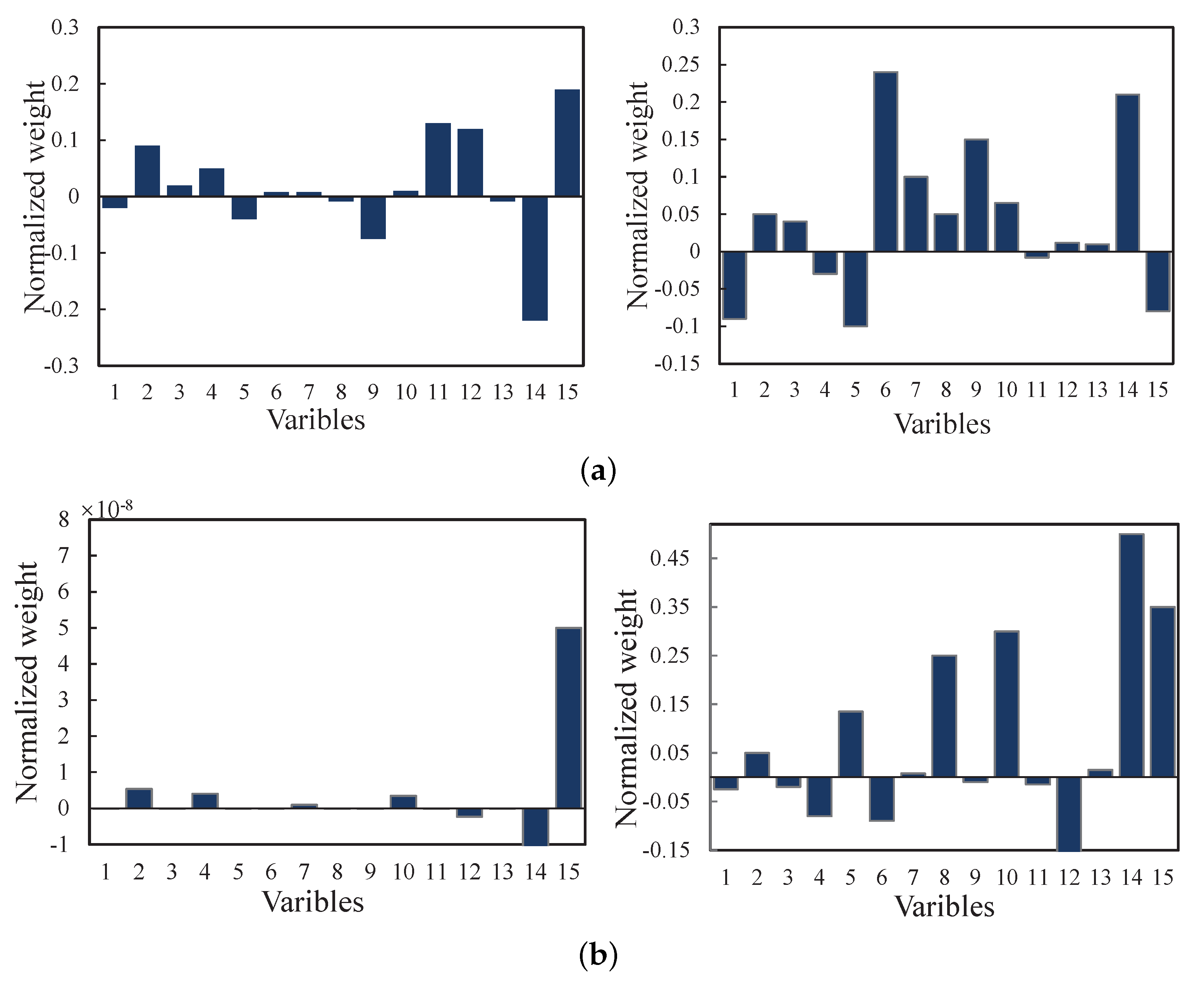
• The least absolute shrinkage and selection operator (LASSO) is used to select the responsible variables for SELFDA model effectively. Then the sparse discriminant optimization problem is formulated and solve by minimization-maximization method. Thus, the data characteristics can be well exploited from the variable dimension.
• Besides, the matrix exponential strategy is integrated into the framework of LFDA. As a consequence, the SELFDA method can function well when encountering the common SSS problem in despite of the dimensions of the input samples.
• Although SELFDA is an LFDA-based method, it is able to jointly overcome the two limitations of conventional LFDA. Thus, SELFDA is more feasible and universal in engineering practices. To our best knowledge, this paper is also the first time to leverage the SELFDA for fault classification of real-world diesel engine.

The outline of this work is structured as below. In Section 2, the classic LFDA model is reviewed. The motivation of this study as well as the specific description of the proposed SELFDA algorithm is presented in detail in Section 3. Simulation experiments are conducted on a simulation process and a real-world diesel working process in Section 4. Finally, conclusions are made in Section 5.

2. Revisit of LFDA

Assume the $X_L=\{x_1,x_2,\dots ,x_l\}\in R^{m\times l}$ is the labeled dataset matrix, where the vector $x_i$ is from m-dimensional space $R^m$. And we assume that there are $n_k$ labeled samples in the kth ($1\le k\le K$) class $C_k$.

Let $S_b$ and $S_w$ be the between-class scatter matrix and within-class scatter matrix. In order to better understand LFDA, the pairwise manner of FDA [18] is the necessary prerequisite knowledge.

$$\begin{array}{cc}\hfill & S_b=\frac{1}{2}\sum _{i=1}^n\sum _{j=1}^n{W}_{i,j}^b\left(x_i-x_j\right){\left(x_i-x_j\right)}^{\mathrm{T}}\hfill \end{array}$$

(1)

$$\begin{array}{cc}& S_w=\frac{1}{2}\sum _{i=1}^n\sum _{j=1}^n{W}_{i,j}^w\left(x_i-x_j\right){\left(x_i-x_j\right)}^{\mathrm{T}}.\hfill \end{array}$$

(2)

where

$$\begin{array}{cc}\hfill & W_{i,j}^b=\left\{\begin{array}{ll}\frac{1}{n}-\frac{1}{n_k}\hfill & \mathrm{if} x_i\in C_k,x_j\in C_k\\ \frac{1}{n}\hfill & \mathrm{otherwise}\end{array}\right.\hfill \end{array}$$

(3)

$$\begin{array}{cc}\hfill & W_{i,j}^w=\left\{\begin{array}{ll}\frac{1}{n_k}\hfill & \mathrm{if} x_i\in C_k,x_j\in C_k\\ 0\hfill & \mathrm{otherwise}\end{array}\right..\hfill \end{array}$$

(4)

Based on the pairwise forms of FDA, the pairwise forms of LFDA can be rewritten as below [11]:

$$\begin{array}{c}\hfill \begin{array}{cc}\hfill & S_{lb}=\frac{1}{2}\sum _{i=1}^n\sum _{j=1}^n{W}_{i,j}^{lb}(x_i-x_j){(x_i-x_j)}^{\mathrm{T}}\hfill \\ \hfill & S_{lw}=\frac{1}{2}\sum _{i=1}^n\sum _{j=1}^n{W}_{i,j}^{lw}(x_i-x_j){(x_i-x_j)}^{\mathrm{T}}.\hfill \end{array}\end{array}$$

(5)

The weighting matrices $W_{i,j}^{lb}$ and $W_{i,j}^{lw}$ are given as

$$\begin{array}{cc}\hfill & W_{i,j}^{lb}=\left\{\begin{array}{ll}{A}_{i,j}\left(\frac{1}{n}-\frac{1}{n_k}\right)\hfill & \mathrm{if} x_i\in C_k,x_j\in C_k\\ \frac{1}{n}\hfill & \mathrm{otherwise}\end{array}\right.\hfill \end{array}$$

(6)

$$\begin{array}{cc}\hfill & W_{i,j}^{lw}=\left\{\begin{array}{ll}\frac{A_{i,j}}{n_k}\hfill & \mathrm{if} x_i\in C_k,x_j\in C_k\\ 0\hfill & \mathrm{otherwise}.\end{array}\right.\hfill \end{array}$$

(7)

where $A_{i,j}$ is the $(i,j)$th element of affinity matrix A, being the affinity between the ith sample and jth sample. Then the projection vectors of LFDA are obtained by the objective function described as below.

$$\begin{array}{c}\hfill J_{\mathrm{LFDA}}=arg\underset{v_{l,i\ne 0}}{max}\left\{\frac{v_{l,i}^{\mathrm{T}}{S}_{lb}{v}_{l,i}}{v_{l,i}^{\mathrm{T}}{S}_{lw}{v}_{l,i}}\right\}.\end{array}$$

(8)

where $v_{l,i}$ represents the i-th discriminant vector in LFDA. It has already been proved that the solution of the above optimization problem is given by:

$$S_{lw}^{-1}{S}_{lb}{w}_{l,i}={\lambda }_{l,i}{w}_{l,i}.$$

(9)

where ${\lambda }_{l,i},w_{l,i},i=1,2,\dots ,m$ are the generalized eigenvalues and corresponding eigenvectors, respectively.

3. Methodology

3.1. Problem Statement and Motivation

Statement and Motivation 1: Generally speaking, there are always plentiful variables in real cases, especially in the complex industrial process, often resulting in inaccurate classification models. To improve the suboptimal classification performance caused by imbalanced number of normal and faulty samples, the model should explore the useful discriminant information and manifold structures from both the labeled and unlabeled samples, which is beneficial for fault classification.

However, most of the exciting LFDA models are unable to carry out variable selection in fault diagnosis area, which incorporates all process variables without emphasizing the key faulty ones. Therefore, the LASSO method is used to select the responsible variables for SELFDA model effectively. Then the sparse discriminant optimization problem is formulated and solve by feasible gradient direction method. Thus, the data characteristics can be well exploited from the variable dimension.

Statement and Motivation 2: Since the within class matrix $S_{lw}$ of LFDA is non-invertible when encounter the frequent SSS problem, thus the discriminant information corresponding to the eigenvalues of $S_{lw}$ that are equal to 0 has been ignored by LFDA, hence the LFDA cannot be applied to the SSS case. As a consequence, the application scope of fault classification methods that developed upon LFDA is largely narrowed, which has brought bottlenecks to the popularizations and implement of these methods in actual industrial process. Therefore, an efficient LFDA-based classification model able to cope with the SSS problem is badly needed.

As described in former sections, if the dimension of dataset exceeds the number of samples, then the $S_{lw}$ in (9) is non-invertible. Thus, the optimization problem of (8) is unsolvable and the fault cannot be accurately classified through the LFDA-based methods. Actually, the SSS problem is quite common in the complex industrial process since the faulty samples are insufficient and hard to obtain in most cases. Therefore, to alleviate the SSS problem is imperative for fault classification models. In the proposed method, the matrix exponential strategy is carried out to develop the favorable model, which can completely solve the SSS issue without reducing the data dimensionality compulsively, and more practical and robust in practical applications. What is more, it also inherits the discriminant nature from LFDA and allows for the enhanced classification performance by the distance diffusion mapping.

3.2. SELFDA

(1) Sparse Local Fisher Discriminant Analysis (SLFDA): Based on LFDA, SLFDA with LASSO sparsity makes the model more concise and interpretable, the object function (9) can be reformulated as below:

$$\begin{array}{cc}\hfill & \underset{{\widehat{w}}_k}{max}{\widehat{w}}_k^{\mathrm{T}}{\widehat{S}}^b{\widehat{w}}_k\hfill \\ \hfill & \mathrm{s}.\mathrm{t}.{\widehat{w}}_k^{\mathrm{T}}{\widehat{S}}^w{\widehat{w}}_k\le 1\hfill \\ \hfill & {\widehat{w}}_k^{\mathrm{T}}{\widehat{S}}^w{\widehat{w}}_i=0(\forall i<k).\hfill \end{array}$$

(10)

where ${\widehat{w}}_k$ is the kth discriminant direction of SLFDA.

The LFDA model can realize variable selection through adding L0 penalty term, which is a NP-hard problem. So the LFDA in (10) can be reformulated by adding LASSO penalty as follows:

$$\begin{array}{cc}\hfill & \underset{{\widehat{w}}_k}{max}{\widehat{w}}_k^{\mathrm{T}}{\widehat{S}}^b{\widehat{w}}_k-\lambda \left|\right|{\widehat{w}}_k{\left|\right|}_1\hfill \\ \hfill & \mathrm{s}.\mathrm{t}.{\widehat{w}}_k^{\mathrm{T}}{\widehat{S}}^w{\widehat{w}}_k\le 1\hfill \\ \hfill & {\widehat{w}}_k^{\mathrm{T}}{\widehat{S}}^w{\widehat{w}}_i=0(\forall i<k).\hfill \end{array}$$

(11)

where $\lambda$ is the LASSO penalty factor. In general, the interpretability and discriminant performance of SLFDA model increase with the increase of $\lambda$ within a certain range, and then decrease.

(2) Solution of SLFDA: As orthogonal constraint in (11) is difficult to satisfy directly. Aiming at this problem, a new between class scatter matrix ${\widehat{S}}_k^b$ is designed to replace ${\widehat{S}}^b$. So that the kth discriminant direction can be calculated as ${\widehat{S}}_k^b={\mathsf{\Psi }}^{\mathrm{T}}{P}_k^{\perp }\mathsf{\Psi }$. If $k=1$, let $P_1^{\perp }=I$, then ${\widehat{S}}_1^b={\widehat{S}}^b$. Or else, the ${\widehat{S}}^b$ can be expressed as ${\widehat{S}}^b={\mathsf{\Psi }}^{\mathrm{T}}\mathsf{\Psi }$ through Cholesky decomposition. Then, a new orthogonal projection matrix $M_k^{\perp }$ projects onto the space that orthogonal to $\mathsf{\Psi }{w}_i$ ($i=1,2,\dots ,k-1$), which can be written as:

$$\begin{array}{c}\hfill M_k^{\perp }=I-\mathsf{\Psi }W{\left(\mathsf{\Psi }W\right)}^{+}.\end{array}$$

(12)

where $W=[{\widehat{w}}_1,{\widehat{w}}_2,\dots ,{\widehat{w}}_{k-1}]$, ${\left(\mathsf{\Psi }W\right)}^{+}$ is the Moore Penrose pseudoinverse of $\mathsf{\Psi }W$.

Generally speaking, problem (11) can be worked out by Lagrangian multiplier regardless of the LASSO penalty as

$$\begin{array}{c}\hfill {\widehat{S}}_k^b{\widehat{w}}_k={\lambda }_k{\widehat{S}}^w{\widehat{w}}_k.\end{array}$$

(13)

And Equation (13) can be turn into the following form by multiplying ${\widehat{w}}_i^{\mathrm{T}}$

$$\begin{array}{c}\hfill {\widehat{w}}_i^{\mathrm{T}}{\widehat{S}}_k^b{\widehat{w}}_k={\lambda }_k{\widehat{w}}_i^{\mathrm{T}}{\widehat{S}}^w{\widehat{w}}_k.\end{array}$$

(14)

Then, the left part of (14) can be changed into

$$\begin{array}{c}\hfill {\widehat{w}}_i^{\mathrm{T}}{\widehat{S}}_k^b{\widehat{w}}_k={\left(\mathsf{\Psi }{\widehat{w}}_i\right)}^{\mathrm{T}}\{I-\mathsf{\Psi }W{\left[{\left(\mathsf{\Psi }W\right)}^{\mathrm{T}}\mathsf{\Psi }W\right]}^{-1}{\left(\mathsf{\Psi }W\right)}^{\mathrm{T}}\}\mathsf{\Psi }{\widehat{w}}_k.\end{array}$$

(15)

Set $m_i=\mathsf{\Psi }{\widehat{w}}_i$, so $m_i^{\mathrm{T}}{m}_i={\widehat{w}}_i^{\mathrm{T}}{\widehat{S}}^b{\widehat{w}}_i={\lambda }_i{\widehat{w}}_i^{\mathrm{T}}{\widehat{S}}^w{\widehat{w}}_i={\lambda }_i$, and $m_i^{\mathrm{T}}{m}_j=0$ when $i\ne j$. Set $M=\mathsf{\Psi }W$, then $M=[m_1,m_2,\dots ,m_{k-1}]$. Therefore, Equation (15) can be changed into (16)

$$\begin{array}{c}\hfill {\lambda }_k{\widehat{w}}_i^{\mathrm{T}}{\widehat{S}}^w{\widehat{w}}_k=[m_i^{\mathrm{T}}-m_i^{\mathrm{T}}M{\left(M^{\mathrm{T}}M\right)}^{-1}{M}^{\mathrm{T}}]m_k.\end{array}$$

(16)

Since ${\left(M^{\mathrm{T}}M\right)}^{-1}$ in (16) is diagonal matrix that consist of $\frac{1}{{\lambda }_i}$, so $m_i^{\mathrm{T}}M{\left(M^{\mathrm{T}}M\right)}^{-1}{M}^{\mathrm{T}}$ can be expressed as:

$$\begin{array}{c}\hfill [0,\dots ,{\lambda }_i,\dots ,0]\left(\begin{array}{cc}1/{\lambda }_1& \\ & \ddots & \\ & & 1/{\lambda }_{k-1}\end{array}\right)\left(\begin{array}{c}{m}_1^{\mathrm{T}}\\ m_2^{\mathrm{T}}\\ ⋮\\ m_{k-1}^{\mathrm{T}}\end{array}\right)=m_i^{\mathrm{T}}.\end{array}$$

(17)

Then we have ${\lambda }_k{\widehat{w}}_i^{\mathrm{T}}{\widehat{S}}^w{\widehat{w}}_k=0$, that is to say ${\widehat{w}}_i^{\mathrm{T}}{\widehat{S}}^w{\widehat{w}}_k=0$. After that, Equation (11) can be calculate as

$$\begin{array}{cc}\hfill & \underset{{\widehat{w}}_k}{max}{\widehat{w}}_k^{\mathrm{T}}{\widehat{S}}_k^b{\widehat{w}}_k-\lambda \left|\right|{\widehat{w}}_k{\left|\right|}_1\hfill \\ \hfill & \mathrm{s}.\mathrm{t}.{\widehat{w}}_k^{\mathrm{T}}{\widehat{S}}^w{\widehat{w}}_k\le 1.\hfill \end{array}$$

(18)

since the problem in (18) is non-convex. And the minimization-maximization (MM) method that is a common choice for figuring out nonconvex functions. Thus, (18) is finally transformed into the following iterative optimization problem by MM algorithm:

$$\begin{array}{cc}\hfill & \underset{\theta }{max}{\theta }^{\mathrm{T}}{\widehat{S}}_k^b{\widehat{w}}_k^i-{\lambda \left|\right|\theta \left|\right|}_1\hfill \\ \hfill & \mathrm{s}.\mathrm{t}.{\theta }^{\mathrm{T}}{\widehat{S}}^w\theta \le 1.\hfill \end{array}$$

(19)

where $\theta$ is the parameter vector used to maximize the objective function. ${\widehat{w}}_k^i$ is the optimal solution of the last iteration. In this way, the kth discriminant direction can be approximated by iterated operation, which can be solved by the feasible gradient direction method [15].

Then, the regularized forms of scatter matrixes $S_{rlb}$ and $S_{rlw}$ are defined in following form:

$$\begin{array}{c}\hfill \begin{array}{cc}\hfill & S_{rlb}=(1-\beta ){\widehat{S}}_k^b+\beta S_t.\hfill \\ \hfill & S_{rlw}=(1-\beta ){\widehat{S}}^w+\beta I_m.\hfill \end{array}\end{array}$$

(20)

where $S_t$ is the total scatter matrix of the whole dataset [18], $I_m$ is an identity matrix, and $\beta \in [0,1]$ denotes the weighting factor. Under most condition, one may choose different $\beta$ value to increase the flexibility of the model.

(3) Derivation Procedure of SELFDA: In order to extract the discriminant information contained in the null space of within-class scatter matrix, the matrix exponential strategy is carried out here. Analogous to the kernel methods, in SELFDA model, suppose there is a non-linear distance diffusion mapping $\phi$, then the scatter matrices $S_{rlb}$ and $S_{rlw}$ can be mapped into a new high-dimensional space.

$$\begin{array}{c}\hfill \phi :R^n\to F\end{array}$$

(21)

$$\begin{array}{c}\hfill S_{rlb}\to \phi \left(S_{rlb}\right)=exp\left(S_{rlb}\right).\end{array}$$

(22)

$$\begin{array}{c}\hfill S_{rlw}\to \phi \left(S_{rlw}\right)=exp\left(S_{rlw}\right).\end{array}$$

(23)

Specifically, taking the covariance matrix $S_{rlb}$ as an example, its exponential form can be calculated as below:

$$\begin{array}{c}\hfill exp\left(S_{rlb}\right)=\mathrm{I}+S_{rlb}+\frac{S_{rlb}^2}{2!}+\cdots =Q{e}^{\wedge }Q.\end{array}$$

(24)

where $S_{rlb}=Q\wedge Q^{\mathrm{T}}$, Q is an orthogonal matrix and ∧ is a diagonal matrix.

Similar to the LFDA introduced in Section 2, the projection directions of SELFDA can be obtained by solving the exponential of $S_{rlb}$ and $S_{rlw}$ from the following optimization problem:

$$J_{\mathrm{SELFDA}}=arg\underset{v_{ce,i\ne 0}}{max}\left\{\frac{v_{ce,i}^{T}exp\left(S_{rlb}\right)v_{ce,i}}{v_{ce,i}^{T}exp\left(S_{rlw}\right)v_{ce,i}}\right\}.$$

(25)

And the matrices $S_{rlb}$ and $S_{rlw}$ should be normalized beforehand to prevent the appearance of large values of the numbers originating from $exp\left(S_{rlb}\right)$ and $exp\left(S_{rlw}\right)$. Since the $exp\left(S_{rlb}\right)$ and $exp\left(S_{rlw}\right)$ are full-rank matrices according to the Theorem 3 in [23]. Thus, the SSS problem of LFDA is solved because there is no need for (25) to consider the singularity of within-class scatter matrix.

Similarly, the solution of (25) is acquired through the following Lagrangian multiplier method:

$$exp\left(S_{rlb}\right)w_{ce,i}={\lambda }_{ce,i}exp\left(S_{rlw}\right)w_{ce,i}.$$

(26)

where ${\lambda }_{ce,i}$ and $w_{ce,i}$ are the eigenvalues and the corresponding eigenvectors, respectively. The first d eigenvectors $W_d=[w_{ce,1},\dots ,w_{ce,d}]$ are used to span the subspace.   

3.3. Discriminant Power of SELFDA

It is noted that SELFDA is equivalent to transforming the original data into a new space by exponential mapping, after that, the LFDA model with comprehensive sample information is carried out in such a new space, which might shown some analogous characteristics of kernel mapping. The only difference between them is that the latter maps the feature vectors while the SELFDA maps the scatter matrices. After that, the SELFDA may show enhanced performance over LFDA when involving nonlinear circumstance.

The LFDA tends to search the optimal discriminate direction, which can minimize the within-class distance and maximize the between-class distance simultaneously. In mathematics, the $trace$ of the scatter matrices can be given:

$$\begin{array}{c}\hfill \begin{array}{c}trace\left(S_{rlb}\right)={\displaystyle \sum _{i=1}^K}{n}_k{∥\left({\mu }_k-\mu \right)∥}_2^2\hfill \\ ={\lambda }_{rlb,1}+{\lambda }_{rlb,2}+\cdots +{\lambda }_{rlb,m}.\hfill \end{array}\end{array}$$

(27)

$$\begin{array}{c}\hfill \begin{array}{c}trace\left(S_{rlw}\right)={\displaystyle \sum _{k=1}^K}{\displaystyle \sum _{x_i\in C_k}}{∥\left(x_i-{\mu }_k\right)∥}_2^2\hfill \\ ={\lambda }_{rlw,1}+{\lambda }_{rlw,2}+\cdots +{\lambda }_{rlw,m}.\hfill \end{array}\end{array}$$

(28)

Since the eigenvalues of $trace\left(S_{rlb}\right)$ are often used to describe the separation between classes, while the eigenvalues of $trace\left(S_{rlw}\right)$ are often used to describe the closeness of the samples within classes. Hence, the discriminant vector that corresponds to the bigger ratio of ${\lambda }_{rlb,i}/{\lambda }_{rlw,i}$ owns stronger discriminant power.

And the eigenvalue of the exponential matrix can be obtained by the following equation:

$$\begin{array}{c}\hfill exp\left(S_{rlb}\right)w_{rlb}=\mathrm{I}{w}_{ce}+S_{rlb}{w}_{rlb}+\cdots =e^{{\lambda }_{rlb}}{w}_{rlb}.\end{array}$$

(29)

where $w_{rlb}$ is the eigenvector of $S_{rlb}$, and ${\lambda }_{rlb}$ is its corresponding eigenvalue.

Therefore, the $trace$ of the SELFDA can be calculated as following:

$$\begin{array}{cc}\hfill trace\left(exp\left(S_{rlb}\right)\right)& =e^{{\lambda }_{rlb,1}}+\cdots +e^{{\lambda }_{rlb,m}}\hfill \\ \hfill trace\left(exp\left(S_{rlw}\right)\right)& =e^{{\lambda }_{rlw,1}}+\cdots +e^{{\lambda }_{rlw,m}}.\hfill \end{array}$$

(30)

It is noticeable that for most of the eigenvalues in (29) and (30), we have the inequality ${\lambda }_{rlb,i}>{\lambda }_{rlw,i}$ and $e^{{\lambda }_{rlb,i}}>e^{{\lambda }_{rlw,i}}$.

Since ${\lambda }_{rlb,i}>{\lambda }_{rlw,i}>0$, then ${\lambda }_{rlb,i}-{\lambda }_{rlw,i}>0$ and consequently since $\forall a>0,e^a>1+a$, we have

$$e^{{\lambda }_{rlb,i}-{\lambda }_{rlw,i}}>1+{\lambda }_{rlb,i}-{\lambda }_{rlw,i}.$$

(31)

Also we have $1+{\lambda }_{rlb,i}-{\lambda }_{rlw,i}>1+\frac{{\lambda }_{rlb,i}-{\lambda }_{rlw,i}}{{\lambda }_{rlw,i}}$, since ${\lambda }_{rlw,i}>1$ for large eigenvalues. We obtain the following equation through transitivity

$$e^{{\lambda }_{rlb,i}-{\lambda }_{rlw,i}}>1+{\lambda }_{rlb,i}-{\lambda }_{rlw,i}>\frac{{\lambda }_{rlb,i}}{{\lambda }_{rlw,i}}.$$

(32)

That gives us

$$\frac{e^{{\lambda }_{rlb,i}}}{e^{{\lambda }_{rlw,i}}}=e^{{\lambda }_{rlb,i}-\lambda rlw,i}>\frac{{\lambda }_{rlb,i}}{{\lambda }_{rlw,i}}.$$

(33)

From the above analysis, we know that diffusion scale to between class distance is bigger than that of within class. That is means, SELFDA can enlarge the margin between different categories compared with LFDA, which is desirable for fault classification.

In order to better understand the working process of SELFDA algorithm, the pseudo-codes are given in Algorithm 1.

Algorithm 1 SELFDA

Input: Training data $X\in R^{m\times n}$ Output: The data matrix projection 1: Establish the of SELFDA model according to (10)–(20) 2: for $i,j=1$ to n, $\beta \in [0,1]$ do 3:     $S_{lb}\leftarrow \frac{1}{2}{\displaystyle \sum _{i=1}^n}{\displaystyle \sum _{j=1}^n}{W}_{i,j}^{lb}(x_i-x_j){(x_i-x_j)}^{\mathrm{T}}$ 4:     $S_{lw}\leftarrow \frac{1}{2}{\displaystyle \sum _{i=1}^n}{\displaystyle \sum _{j=1}^n}{W}_{i,j}^{lw}(x_i-x_j){(x_i-x_j)}^{\mathrm{T}}$ 5:     $S_{rlb}\leftarrow (1-\beta ){\widehat{S}}_k^b+\beta S_t$ 6:     $S_{rlw}\leftarrow (1-\beta ){\widehat{S}}^w+\beta I_m$ 7: Implement the matrix exponential on $S_{rlb}$ and $S_{rlw}$ to construct the optimization problem of (25) 8: $\{{\lambda }_{ce,i},w_{ce,i}\}\leftarrow$ Solve the optimization problem in (25) by $exp\left(S_{rlb}\right)w_{ce,i}={\lambda }_{ce,i}exp\left(S_{rlw}\right)w_{ce,i}$ 9: Rank the eigenvectors $w_{ce,i}$ according to the eigenvalues ${\lambda }_{ce,i}$ in descending order 10: end for 11: for $d<n$  do 12: Choose the first d eigenvectors associated with the first d eigenvalues defined by $W_d=[w_{ce,1},\dots ,w_{ce,d}]$ 13: end for 14: The projection of X into the discriminant subspace is given by $W_d^{\mathrm{T}}X$

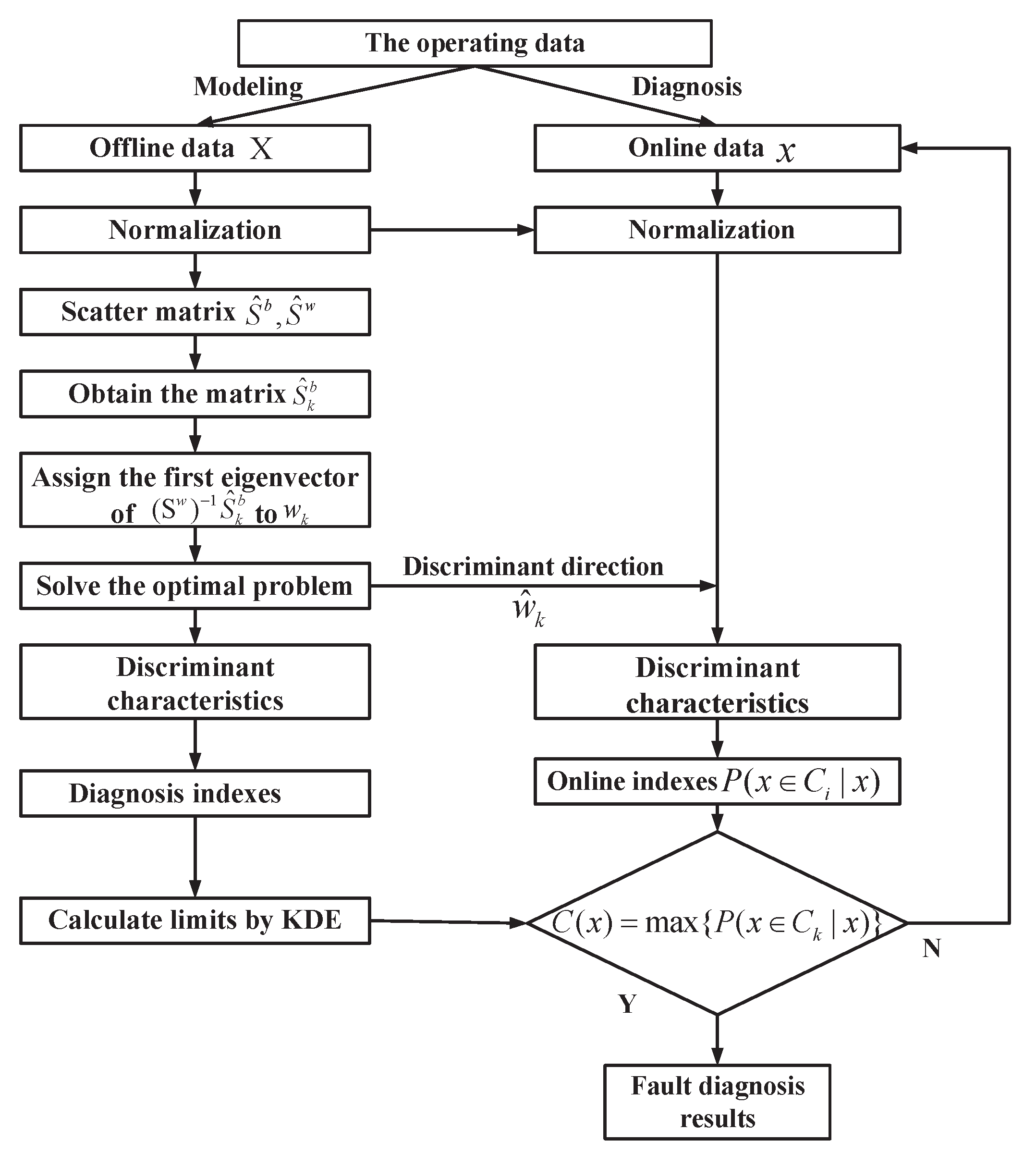
3.4. SELFDA-Based Fault Diagnosis Scheme

After introducing the theoretical framework of SELFDA, the Bayesian inference is borrowed to realize fault classification. Suppose all the samples follow the Gaussian distributions and thereby the priori probability of each category is $P\left(x\in C_k\right)=\frac{1}{K}$. Hence, the conditional probability density function (PDF) of the new testing sample x is given as:

$$\begin{array}{c}\hfill \begin{array}{cc}\hfill & P\left(x|x\in C_k\right)=\frac{exp\left[-\frac{{\left(x-{\overline{x}}_k\right)}^{\mathrm{T}}{W}_d{\Sigma }_k^{-1}{W}_d^{\mathrm{T}}\left(x-{\overline{x}}_k\right)}{2}\right]}{{\left(2\pi \right)}^{d/2}det{\left[\left({\Sigma }_k\right)\right]}^{1/2}}\hfill \\ \hfill & {\Sigma }_k=\frac{1}{n_k-1}{W}_d^{\mathrm{T}}exp\left(S_k\right)W_d.\hfill \end{array}\end{array}$$

(34)

where ${\overline{x}}_k$ and $S_k$ are the mean vector and within-class scatter matrix of the labeled training dataset in $C_k$. $W_d$ is a matrix used for dimensionality reduction of the data. In the light of Bayes rule, the posterior probability of the x belonging to ith fault category is expressed as:

$$P\left(x\in C_k|x\right)=\frac{P\left(x|x\in C_k\right)P\left(x\in C_k\right)}{{\sum }_{i=1}^{K}P\left(x|x\in C_k\right)P\left(x\in C_k\right)}.$$

(35)

As a result, the testing samples are classified into the certain type by the classification criterion defined in (36).

$$\begin{array}{c}\hfill C\left(x\right)=arg\underset{1\le k\le K}{max}\left\{P\left(x\in C_k|x\right)\right\}.\end{array}$$

(36)

To simplify the discriminant task in practice, a discriminant function can be redefined as follows

$$g_k\left(x\right)=-\frac{{\left(x-{\overline{x}}_k\right)}^{\mathrm{T}}{W}_d{\Sigma }_k^{-1}{W}_d^{\mathrm{T}}\left(x-{\overline{x}}_k\right)}{2}-\frac{ln\left[det\left({\Sigma }_k\right)\right]}{2}.$$

(37)

In conclusion, the flowchart of the favorable SELFDA method is briefly showed in Figure 1.

4. Experimental Results and Discussion

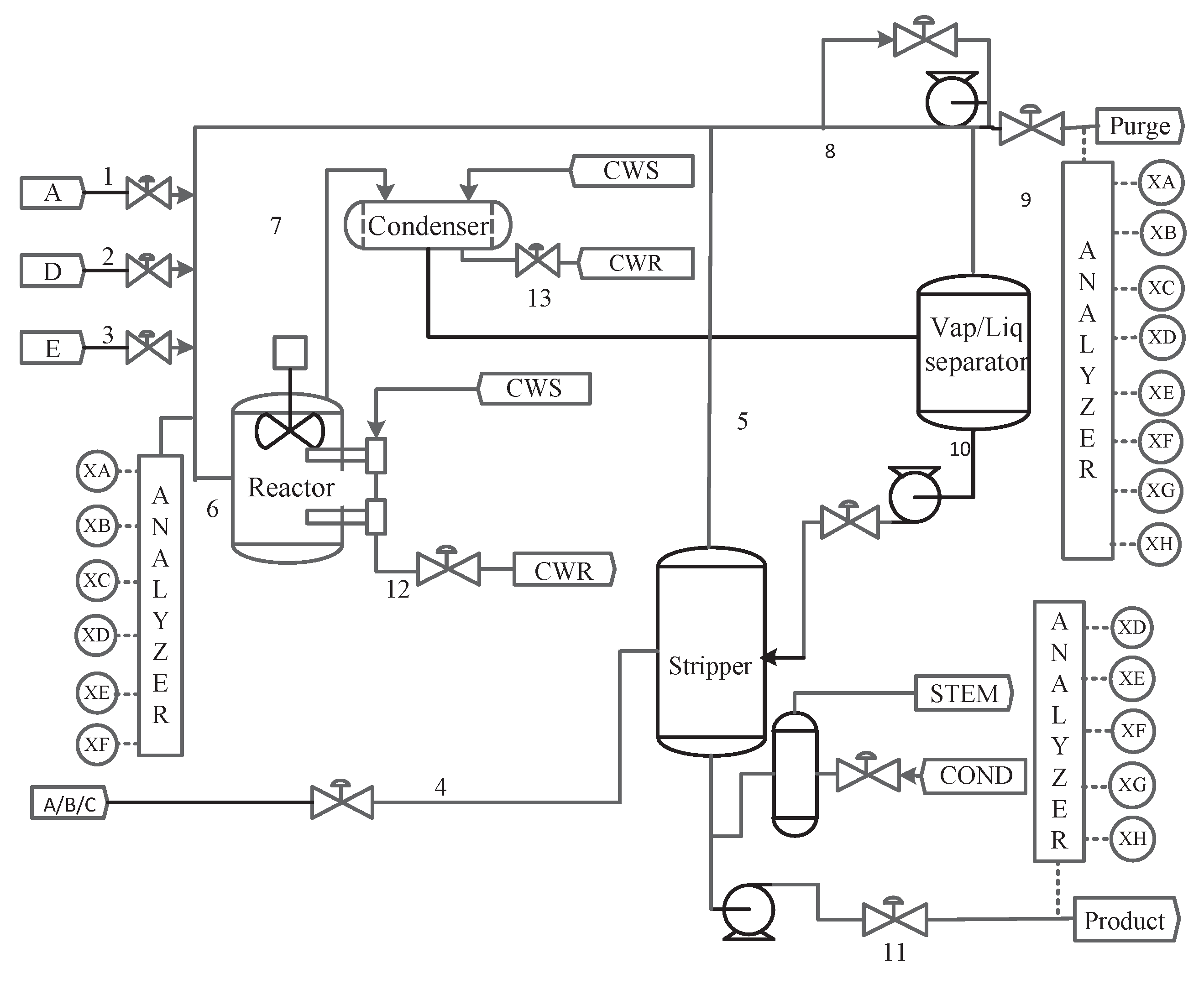
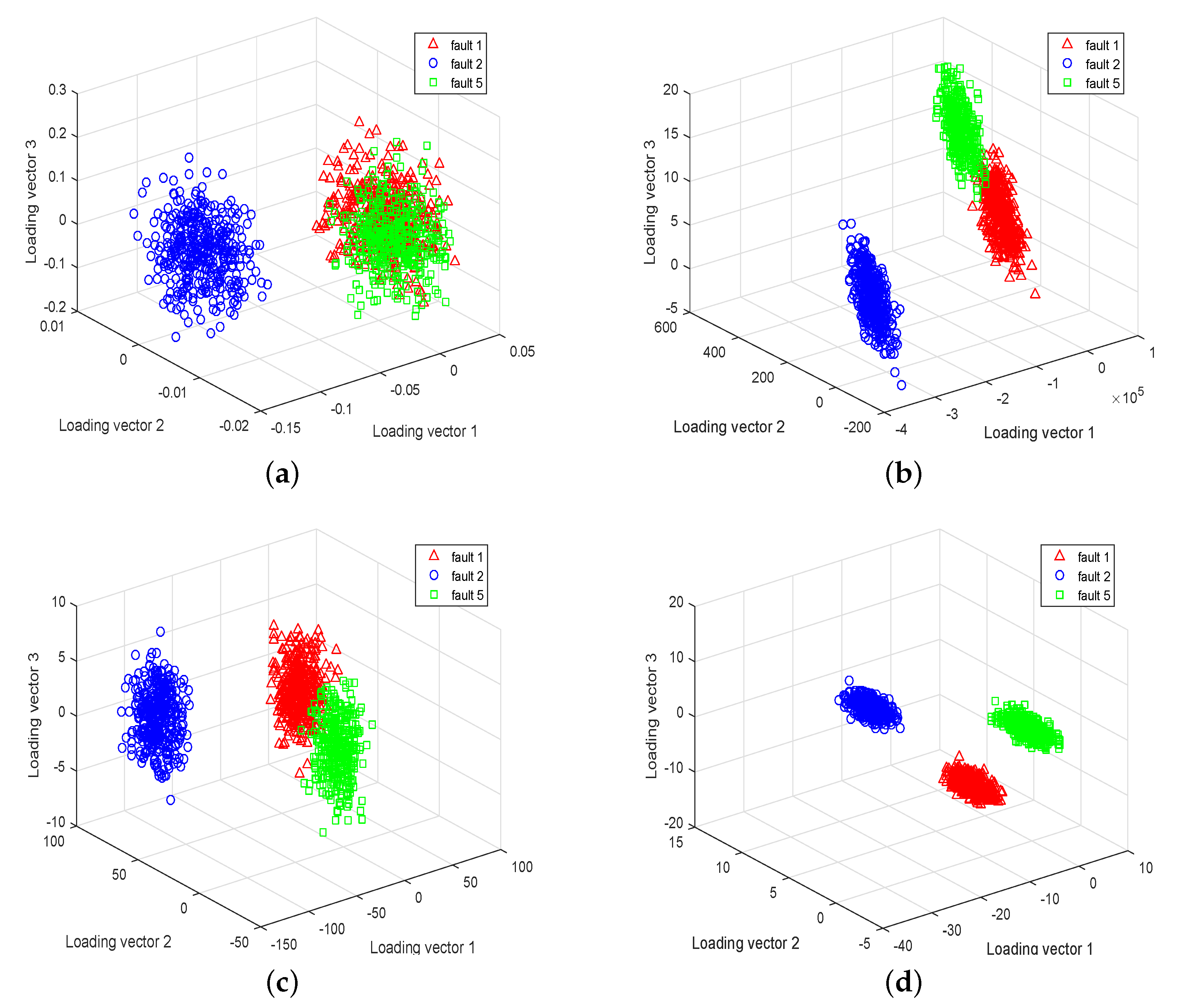
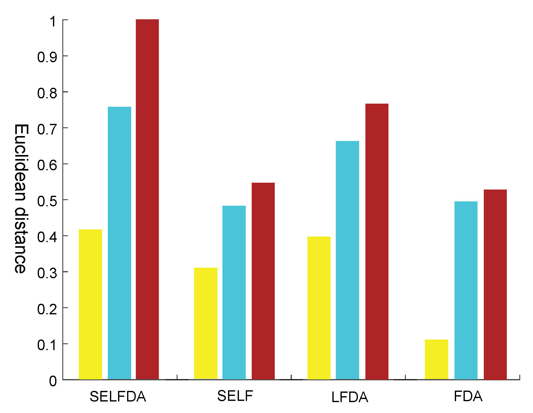
4.1. TE Process

The TE process is a benchmark simulation platform of the real chemical process, which is firstly proposed by Downs and Vogel [27]. It mainly composed of five parts: a reactor, a condenser, a recycle compressor, a separator and a striper. In this process, each sample contains 52 variables, including 12 manipulated variables and 41 measured variables. There are also 21 types of programmed fault conditions. More information about the TE process can refer to [26,28]. The process mainly produces two products with four raw materials. And Figure 2 shows the schematic diagram of the TE process.

In order to carry out the fault classification experiment, all the 41 measurement variables are used in this work, and Faults 1, 2 and 5 are taken as an example to carry out detailed comparative studies between FDA and LFDA, SELF and SELFDA, since they are all step faults involving process variables [18], hence it is suitable to verify the SELFDA in this paper. The description and types of the three faults are showed in

Table 1. Three Faults in The TE Process.

No	Description	Type
Fault 1	A/C feed ratio B composition constant	Step
Fault 2	B composition, A/C ration constant	Step
Fault 5	Condenser cooling water inlet temperature	Step

. Every fault contains 200 samples for training and the labeled samples account for 5% of each class, which are selected randomly. The testing dataset include 1200 faulty samples (each failure contains 400 samples). For convenience, the value of weighting factor parameter $\beta$ is chosen as 0.4.

(1) Analysis of the Visual Performance: To be noted, the classification results obtained by different methods are shown in Figure 3a–d. Specifically, there is plenty of overlaps between Fault 1 and Fault 5 in Figure 3a, that is means, the FDA cannot separate the three faults well. And the similar situation happens in Figure 3b,c. In contrast, from the visual results in Figure 3d, we know that SELFDA method shows no overlaps in separating the three faults, which means the SELFDA achieves best classification performance with least misclassification points. To demonstrate the superiority of SELFDA better, the Euclidean distance between the centers of the three faults in the low-dimensional space are calculated and shown in Figure 4. The bar charts in different colors denote the distances obtained by different faults, and normalized them into [0, 1]. From the figure, it is easy to conclude that the three bar charts achieved by SELFDA is higher than the corresponding ones of the competitors, that is to say, the three faults are farther parted by SELFDA, which verify the classification capacity of SELFDA from another point of view.

(2) Discussions of the Classification Accuracy: Here, we choose accuracy as the performance metric for diagnosis. Accuracy refers to the proportion of correctly classified samples by a classification model among the total number of samples. Furthermore, the quantified classification results of different algorithms are given in

Table 2. Classification Accuracy of The Faults In TE Process.

	FDA	LFDA	SELF	SELFDA
Fault 1	83.25%	83.25%	64%	100%
Fault 2	39.5%	0.95%	100%	100%
Fault 5	63.75%	69.5%	66.5%	96.25%
Average	62.17%	54.08%	76.83%	98.75%

. Both the FDA and LFDA show undesirable performance since none of them can explore the comprehensive discriminant information. The classification performance of SELF is improved to some degree since it involves the whole dataset, however, the SSS problem is not included. By contrast, SELFDA acquires the best classification accuracy (highlighted in bold) regarding Fault 1 (100%), Fault 2 (100%) and Fault 5 (96.25%), respectively. And the average classification accuracy is also the highest (98.75%), which further explained the effectiveness of the SELFDA method. The enhanced discrimination performance of SELFDA over the comparing algorithms can be explained by two reasons. First, SELFDA makes full use of the discrimination information that contained in both the labeled and unlabeled samples. Second, it can enlarge the margins distance between different fault categories after the introduction of matrix exponential strategy.

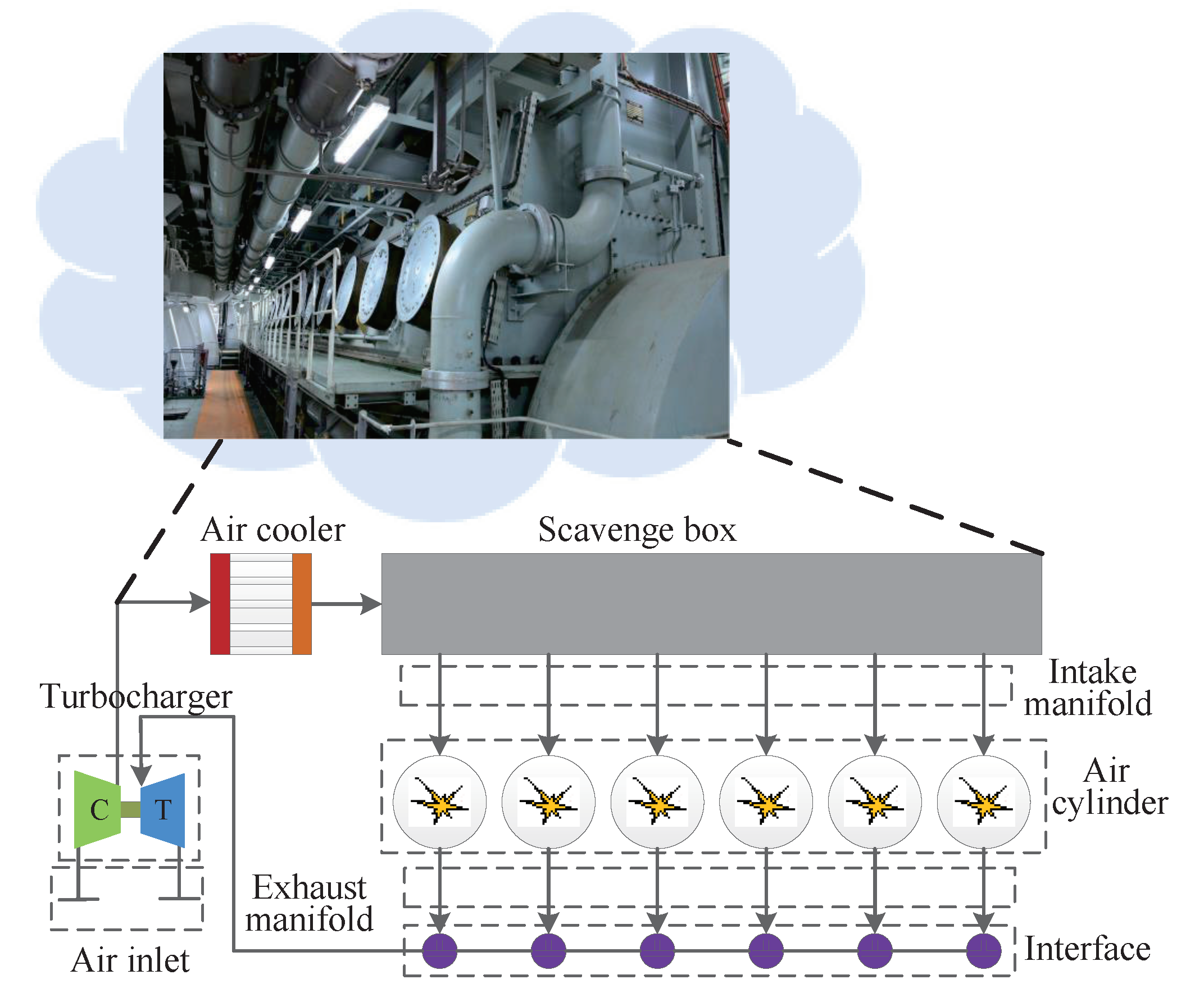
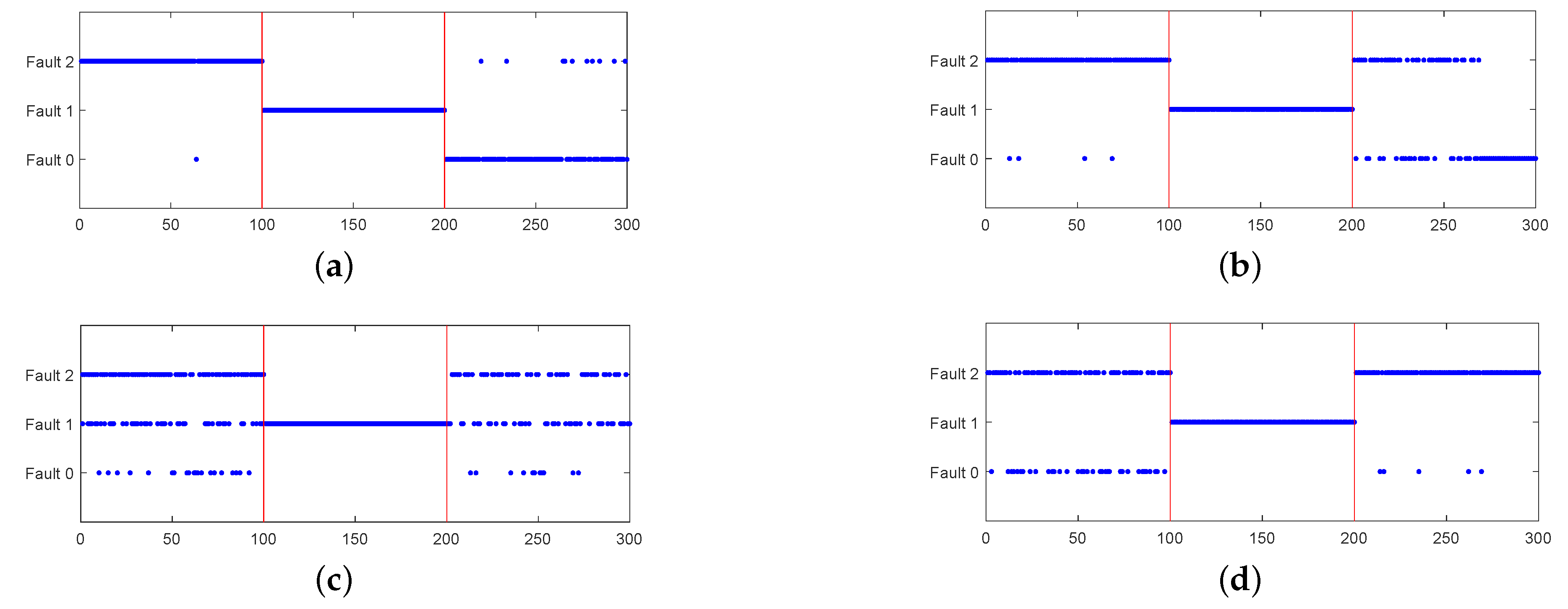
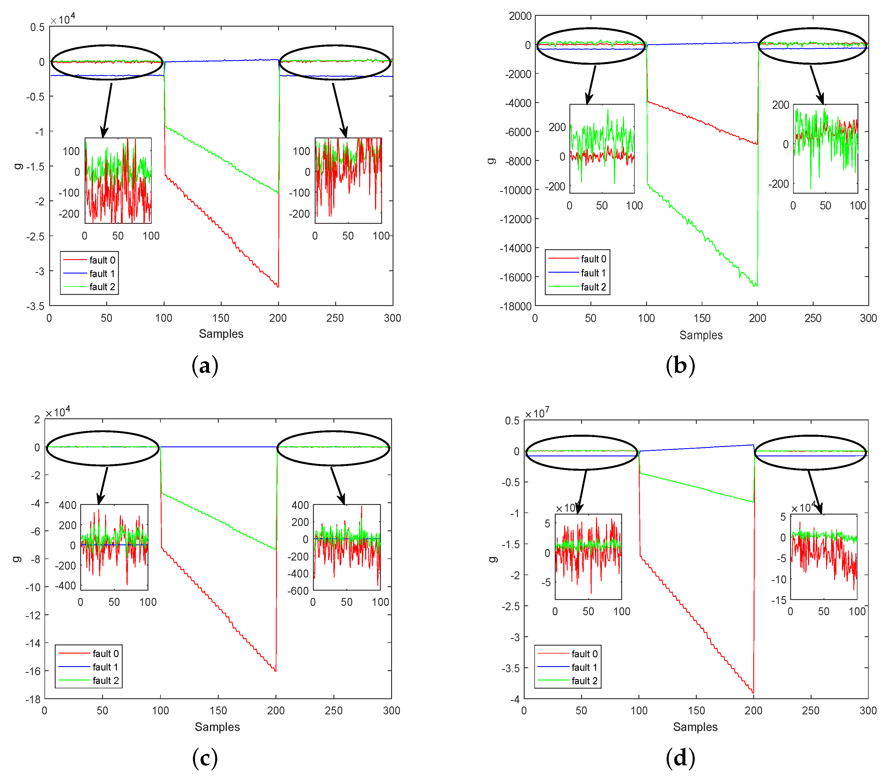
4.2. Real-World Diesel Working Process

Due to the thermal efficiency, long useful life and high reliability of the diesel engine, it has been widely utilized in ships. Nevertheless, since the aging process of the machine is irreversible, the working environment is harsh, and various faults occur frequently, thus resulting in economic losses and even casualties. To this end, ever-increasing attention should be paid to accurate and timely fault diagnosis for diesel engine. And abundant scientific payoffs have been proposed recently from both academia and industry. For example, the authors of [29] analysed the vibration data by artificial neural networks to realize fault classification in a four-stroke gasoline engine. More recently, ref. [30] presented LAMDA algorithm to classify the faults in an automotive diesel engine operating under some smooth operating conditions.

However, in-depth analysis of the above researches, none of them can handle the SSS problem or large number of unlabeled fault samples, which are quite common in diesel working process. In this paper, two universal process failures are used to confirm the superiority of SELFDA in fault classification. One of them is the exhaust pipe blockage (i.e., fault 1), the other is insufficient cooling of the air cooler (i.e., fault 2), all the operating data are collected during the working process of the 6S35ME-B9 diesel engine produced by the MAN company, which is demonstrated in Figure 5, the main system parameters and monitored sensor variables of 6S35ME-B9 diesel engine are given in

Table 3. Main System Parameters of 6S35ME-B9 Diesel Engine.

Parameter	Value	Unit
Rated power	3570	Kw
Rated speed	142	r/min
Cylinders	6	N
Fuel consumption	174.36	g/kw·h
Stroke	2	t
Oil	MGO	-
Viscosity	3–5 at 100 °C	cSt
Density	≤0.887 at 15 °C	g/cm${}^3$

and

Table 4. Monitored Variables in Diesel Engine Working Process.

No.	Variable Description	Units	No.	Variable Description	Units
1	Diesel power	kW	9	Scavenge air pressure	Bar
2	Exhaust manifold pressure	Bar	10	Scavenge air temp	${}^{\circ }\mathrm{C}$
3	Press flow	kg/c	11	Pressure difference	Bar
4	Outlet temp of press	${}^{\circ }\mathrm{C}$	12	Exhaust gas tempe	${}^{\circ }\mathrm{C}$
5	Outlet pressure of press	Bar	13	Exhaust pipe pressure	Bar
6	Intercooler post temp	${}^{\circ }\mathrm{C}$	14	Turbocharger inlet tempe	${}^{\circ }\mathrm{C}$
7	Fuel consumption	g/kw·h	15	Turbocharger outlet tempe	${}^{\circ }\mathrm{C}$
8	Intercooler post pressure	Bar

, respectively. And the detail introduction of the system parameters and data acquisition process can refer to [15].

In this experiment, each type of the faults contains 200 samples and 900 normal samples for training and the labeled samples account for 10% of each class, which are selected randomly. The testing dataset includes 100 normal samples (Fault 0) and 200 faulty samples (each type of fault contains 100 samples). For simplicity, weighting factor parameter $\beta$ is set as 0.5 here. The detailed classification performance of different methods is shown in Figure 6. The horizontal axis denotes the position of the sample points, the first 100 samples are Fault 0, the 101–200th ones are Fault 1, and the last 100 ones are Fault 2, the vertical axis presents the label of the corresponding sample. From Figure 6, all four methods show excellent performance in classifying Fault 1. However, the classification performance of SELFDA is obviously better than the other three methods regarding Fault 0 and Fault 2. This improvement is mainly ascribed to the advantages of SELFDA discussed earlier.

Also, the discriminant functions of different methods are detailedly demonstrated in Figure 7a–d, it is easy to see that the discriminant functions of Fault 1 produced by the four methods own the maximum output in the corresponding interval (100–200th samples), which means all of they can separate Fault 1 well. However, there are a lot of intersections and overlaps between the discriminant function curves of Fault 0 and Fault 2, with a mass of false and missing classified points in all the three contrast algorithms. However, this situation is greatly relieved by SELFDA in Figure 7d, which further exhibit the superiorities of SELFDA in complex industrial processes.

Besides, the quantitative classification results are tabulated in

Table 5. Classification Accuracy of The Faults In Real-Word Diesel Working Process.

	FDA	LFDA	SELF	SELFDA
Fault 0	1%	4%	20%	35%
Fault 1	100%	100%	100%	100%
Fault 2	10%	43%	49%	95%
Average	37%	49%	56.33%	76.67%

. And the highest classification accuracy (in bold) are all achieved by SELFDA (35% for Fault 0, 100% for Fault 1, 95% for Fault 2 and 76.67% for average). More specifically, the classification accuracy produced by SELFDA is 15% and 46% higher than the suboptimal SELF model for Fault 0 and Fault 2, respectively. The average classification accuracy of SELFDA is also significantly enhanced compared to FDA (76.67% versus 37.00%), LFDA (76.67% versus 49%) and SELF (76.67% versus 56.33%).

In addition, normalized weight of each variable regarding fault 1 and fault 2 of the real-word diesel working process obtained by the four methods are given in Figure 8a–d. Specifically, from Figure 8a, we know that the first three key variables of fault 1 are misidentified as variables 11, 14, 15 by FDA. Analogously, the key variables fault 2 are also misidentified as variables 6, 9, 14. And the similar situation happens in Figure 8b since the LFDA approach is unable to handle the variable selection issue. By contrast, SLFDA can recognize the real responsible variables (variables 2, variable 12 for fault 1, variable 7, variable 9 and variable 10 for fault 2) in Figure 8c successfully, which is in consistence with actual condition. Besides, the proposed SELFDA method can also automatically select the key variables for different faults, and the details are demonstrated in Figure 8d.

5. Conclusions

This paper presents an practical SELFDA model, which improves the discrimination performance of conventional LFDA and provides a promising way to handle the challenges of multimodality, model interpretability. Besides, the novel method is insensitive to SSS problem that can enhance the performance of traditional LFDA in real industrial cases. And the simulation results on both the simulated and real industrial process demonstrated that this new fault classification framework outperforms the FDA and LFDA methods. In the future work, embedding the classification method into software systems deserves further explorations.

References

1. Yin, S.; Li, X.; Gao, H.; Kaynak, O. Data-Based Techniques Focused on Modern Industry: An Overview. IEEE Trans. Ind. Electron. 2015, 62, 657–667. [Google Scholar] [CrossRef]
2. Subrahmanya, N.; Shin, Y.C. A data-based framework for fault detection and diagnostics of non-linear systems with partial state measurement. Eng. Appl. Artif. Intell. 2013, 26, 446–455. [Google Scholar] [CrossRef]
3. Chiang, L.H.; Russell, E.L.; Braatz, R.D. Fault Detection and Diagnosis in Industrial Systems; Springer Science & Business Media: Berlin, Germany, 2000. [Google Scholar]
4. Wang, H.; Cai, Y.; Fu, G.; Wu, M.; Wei, Z. Data-driven fault prediction and anomaly measurement for complex systems using support vector probability density estimation. Eng. Appl. Artif. Intell. 2018, 67, 1–13. [Google Scholar] [CrossRef]
5. Tidriri, K.; Tiplica, T.; Chatti, N.; Verron, S. A generic framework for decision fusion in Fault Detection and Diagnosis. Eng. Appl. Artif. Intell. 2018, 71, 73–86. [Google Scholar] [CrossRef]
6. Jiang, Y.; Yin, S. Recent Advances in Key-Performance-Indicator Oriented Prognosis and Diagnosis with a MATLAB Toolbox: DB-KIT. IEEE Trans. Ind. Inform. 2018, 15, 2849–2858. [Google Scholar] [CrossRef]
7. Nor, N.M.; Hassan, C.R.C.; Hussain, M.A. A review of data-driven fault detection and diagnosis methods: Applications in chemical process systems. Rev. Chem. Eng. 2019, 36, 513–553. [Google Scholar] [CrossRef]
8. Jiang, Q.; Yan, X.; Huang, B. Performance-Driven Distributed PCA Process Monitoring Based on Fault-Relevant Variable Selection and Bayesian Inference. IEEE Trans. Ind. Electron. 2016, 63, 377–386. [Google Scholar] [CrossRef]
9. Tong, C.; Lan, T.; Zhu, Y.; Shi, X.; Chen, Y. A missing variable approach for decentralized statistical process monitoring. ISA Trans. 2018, 81, 8–17. [Google Scholar] [CrossRef]
10. Zhao, C.; Gao, F. Critical-to-fault-degradation variable analysis and direction extraction for online fault prognostic. IEEE Trans. Control Syst. Technol. 2017, 25, 842–854. [Google Scholar] [CrossRef]
11. Sugiyama, M. Dimensionality reduction of multimodal labeled data by local fisher discriminant analysis. J. Mach. Learn. Res. 2007, 8, 1027–1061. [Google Scholar]
12. Yu, J. Localized Fisher discriminant analysis based complex chemical process monitoring. AIChE J. 2011, 57, 1817–1828. [Google Scholar] [CrossRef]
13. Yu, J. Nonlinear bioprocess monitoring using multiway kernel localized Fisher discriminant analysis. Ind. Eng. Chem. Res. 2011, 50, 3390–3402. [Google Scholar] [CrossRef]
14. Feng, J.; Wang, J.; Zhang, H.; Han, Z. Fault Diagnosis Method of Joint Fisher Discriminant Analysis Based on the Local and Global Manifold Learning and Its Kernel Version. IEEE Trans. Autom. Sci. Eng. 2016, 13, 122–133. [Google Scholar] [CrossRef]
15. Zhong, K.; Han, M.; Qiu, T.; Han, B. Fault Diagnosis of Complex Processes Using Sparse Kernel Local Fisher Discriminant Analysis. IEEE Trans. Neural Netw. Learn. Syst. 2020, 31, 1581–1591. [Google Scholar] [CrossRef]
16. Liang, M.; Jie, D.; Kaixiang, P.; Chuanfang, Z. Hierarchical Monitoring and Root Cause Diagnosis Framework for Key Performance Indicator-Related Multiple Faults in Process Industries. IEEE Trans. Ind. Inform. 2018, 15, 2091–2100. [Google Scholar]
17. Adeli, E.; Thung, K.H.; An, L.; Wu, G.; Shi, F.; Wang, T.; Shen, D. Semi-supervised discriminative classification robust to sample-outliers and feature-noises. IEEE Trans. Pattern Anal. Mach. Intell. 2019, 41, 515–522. [Google Scholar] [CrossRef]
18. Zhong, S.; Wen, Q.; Ge, Z. Semi-supervised Fisher discriminant analysis model for fault classification in industrial processes. Chemom. Intell. Lab. Syst. 2014, 138, 203–211. [Google Scholar] [CrossRef]
19. Yan, Z.; Huang, C.C.; Yao, Y. Semi-supervised mixture discriminant monitoring for chemical batch processes. Chemom. Intell. Lab. Syst. 2014, 134, 10–22. [Google Scholar] [CrossRef]
20. Liu, J.; Song, C.; Zhao, J. Active learning based semi-supervised exponential discriminant analysis and its application for fault classification in industrial processes. Chemom. Intell. Lab. Syst. 2018, 180, 42–53. [Google Scholar] [CrossRef]
21. Chen, L.F.; Liao, H.Y.M.; Ko, M.T.; Lin, J.C.; Yu, G.J. A new LDA-based face recognition system which can solve the small sample size problem. Pattern Recognit. 2000, 33, 1713–1726. [Google Scholar] [CrossRef]
22. Ye, J.; Li, Q. A two-stage linear discriminant analysis via QR-decomposition. IEEE Trans. Pattern Anal. Mach. Intell. 2005, 27, 929–941. [Google Scholar]
23. Zhang, T.; Fang, B.; Tang, Y.Y.; Shang, Z.; Xu, B. Generalized discriminant analysis: A matrix exponential approach. IEEE Trans. Syst. Man Cybern. Part B (Cybern.) 2009, 40, 186–197. [Google Scholar] [CrossRef]
24. Adil, M.; Abid, M.; Khan, A.Q.; Mustafa, G.; Ahmed, N. Exponential discriminant analysis for fault diagnosis. Neurocomputing 2016, 171, 1344–1353. [Google Scholar] [CrossRef]
25. Dornaika, F.; Bosaghzadeh, A. Exponential local discriminant embedding and its application to face recognition. IEEE Trans. Cybern. 2013, 43, 921–934. [Google Scholar] [CrossRef]
26. Yu, W.; Zhao, C. Recursive Exponential Slow Feature Analysis for Fine-Scale Adaptive Processes Monitoring With Comprehensive Operation Status Identification. IEEE Trans. Ind. Inform. 2019, 15, 3311–3323. [Google Scholar] [CrossRef]
27. Downs, J.J.; Vogel, E.F. A plant-wide industrial process control problem. Comput. Chem. Eng. 1993, 17, 245–255. [Google Scholar] [CrossRef]
28. Tong, C.; Lan, T.; Shi, X. Double-layer ensemble monitoring of non-gaussian processes using modified independent component analysis. ISA Trans. 2017, 68, 181–188. [Google Scholar] [CrossRef]
29. Ahmed, R.; Sayed, M.E.; Gadsden, S.A.; Tjong, J.; Habibi, S. Automotive Internal-Combustion-Engine Fault Detection and Classification Using Artificial Neural Network Techniques. IEEE Trans. Veh. Technol. 2015, 64, 21–33. [Google Scholar] [CrossRef]
30. Ruiz, F.A.; Isaza, C.V.; Agudelo, A.F.; Agudelo, J.R. A new criterion to validate and improve the classification process of LAMDA algorithm applied to diesel engines. Eng. Appl. Artif. Intell. 2017, 60, 117–127. [Google Scholar] [CrossRef]
Figure 1. Flowchart of the SELFDA based fault diagnosis.
Machines 11 01066 g001
Figure 2. The schematic diagram of benchmark TE process.
Machines 11 01066 g002
Figure 3. Classification results by (a) FDA, (b) LFDA, (c) SELF, and (d) SELFDA.
Machines 11 01066 g003
Figure 4. Between-class distances produced by different methods.
Machines 11 01066 g004
Figure 5. Layout and schematic diagram of 6S35ME-B9 diesel engine.
Machines 11 01066 g005
Figure 6. Fault classification performance of testing samples by (a) FDA, (b) LFDA, (c) SELF, and (d) SELFDA.
Machines 11 01066 g006
Figure 7. Discriminant function curve of three faults achieved by (a) FDA, (b) LFDA, (c) SELF, and (d) SELFDA.
Machines 11 01066 g007
Figure 8. Normalized weight of each variable in Fault 1 (left) and Fault 2 (right) of diesel engine working process. (a) FDA, (b) LFDA, (c) SLFDA, (d) SELFDA.
Machines 11 01066 g008aMachines 11 01066 g008b