Abstract
An observer is proposed for a trapezoidal brushless DC motor composed of a cascade connection of a reduced-order Luenberger observer and a high-order sliding mode (HOSM) differentiator. This configuration can estimate the angular velocity and reconstruct the load torque, key elements for the control of this type of motor, under the mild assumption that the variable load torque and its k-th time derivatives are bounded. The proposed observer was tested on an experimental test bench based on Texas Instruments (TI) High Voltage Digital Motor Control (HVMTR Kit) using a Delfino F28379D micro controller. The results show that the velocity and load torque can be properly estimated, despite the presence of noise in the current measurements.
1. Introduction
The Brushless Direct Current motor (BLDC) has become a good choice for variable speed drives, given its simple structure, ruggedness, low cost, high efficiency, and good speed versus torque characteristics, all of them well suited to demanding applications, such as electric vehicles, as indicated in [1,2]. In these applications, it is important to estimate or identify the disturbance, commonly the load torque, to compensate its effect. Most of the recent articles in the study of load torque estimation for electric motors are designed for permanent magnet synchronous motors (PMSM). An example is the work [3], where an improved observer for a surface permanent magnet machine is proposed. This observer utilizes injection-based self-sensing for position, velocity, and disturbance torque estimation. Another example is [4], where the viscous friction coefficient and the moment of inertia are obtained by an extended sliding mode observer and the load torque is identified by a Luenberger observer working in parallel, and results are validated using simulations. The article [5] proposes a double extended sliding-mode observer-based synchronous estimation method of total inertia and load torque for a PMSM in a roller grinding machine, and simulations and experiments are presented to validate the proposed method. More recently, in the article [6] two observers are used, an adaptive-gain super-twisting load torque observer and a variable-learning-rate Adaline inertia observer, with performance validated via simulations and experiments.
In the case of the trapezoidal BLDC motor load estimation, the articles [7,8] present a Generalized Proportional Integral Observer (GPIO) designed to compensate variable lumped disturbances, such as load torque and friction terms. The work [9] studies an Electro–mechanical Actuator (EMA) for aerospace applications which includes a trapezoidal BLDC. The proposed method estimates the residual torque, defined as the sum of all the friction and viscous torques, from data acquired during the functioning of the EMA; simulations are used to validate this scheme. Using another approach, in the work [10] the torque is estimated from real-time data using five distinct Adaptive-Network Based Fuzzy Inference Systems. Finally, the article [11] presents a comparison between Kalman and Extended Kalman Filters algorithms for torque estimation; simulations are also used to validate the proposed approach.
For commutation purposes, BLDC motors are commonly equipped with Hall effect sensors to provide a discrete measure of the angular position, used for back electromotive force versus angular position calculations. These sensors are widely used because of their small volume, light weight and low cost compared with traditional optical or capacitive encoders. Their disadvantage is that after processing the sensor signals, the obtained position is discrete, and its resolution depends on the number of installed sensors. Furthermore, the error in the position may vary depending on whether they are mounted externally or internally, as was found in [12]. To solve this problem, various solutions have been proposed. For example, in [13], a technique is proposed based on a novel dual observer for the estimation of speed and rotor position, which utilizes low-resolution position sensors. In [14] an observer is designed to reconstruct the electrical angular position, while in [15], on the basis of a position error compensator, an online advanced angle adjustment method using input voltage and input current is proposed. More recently, ref. [16] estimates the position using the calculated rotational rotor’s speed and elapsed time.
Therefore, the problem to solve in this paper is the estimation of the torque load, calculated as a variable lumped disturbance, in the rotor shaft of a trapezoidal BLDC motor that uses Hall effect sensors. For this purpose, an interconnected observer [17,18] is applied to the BLDC motor disturbance estimation problem. The observer is formed by the cascade connection of a reduced-order Luenberger observer and a high-order sliding mode (HOSM) differentiator, which reconstructs the disturbance by using the motor model. Unlike several of the works mentioned above, the load torque in this technique may not be constant or a predefined function, but a time-varying function, provided that both the function and its k-th derivatives are bounded. In addition, to complement the cascade observer implementation, a position estimation algorithm (PEA) is designed to obtain the angular position from the Hall effect sensors signals.
To prove the validity of the scheme, first, simulations are performed that can calibrate the experimental platform and give an idea of the expected results. Then, experiments are executed on a commercial platform, composed of a motor equipped with Hall sensors, a power driver, a DC motor, and a standard micro-controller. The main contributions of this article are as follows:
- The proposed method can estimate time-varying load torque, provided that this torque and its k-th derivatives are bounded;
- A position estimation algorithm (PEA) is included to use with Hall effect sensor signals when needed;
- The proposed scheme can guarantee a bounded error in the disturbance estimation, the size of which depends on the measurement noise and sampling time.
The paper is organized as follows. Section 2 recalls the mathematical model of the BLDC motor and the observability definitions needed for the observer design. Section 3 presents the interconnected observer design. Section 4 includes a numerical validation of the observer. Section 5 presents the test bench, the PEA, and the experimental results. Finally, Section 6 contains the conclusions of this work.
2. Preliminaries
This section presents the brushless DC motor model and the basic notions needed for the observer design.
2.1. Brushless DC Motor Model
The brushless DC motor under study has three sets of windings on the inside surface of the stator connected in a Y configuration and a permanent magnet rotor. The magnetic fields in this motor are uniformly distributed, which implies that when the motor is at constant speed, the back electromotive force has a trapezoidal shape. It it is assumed that the stator phases are balanced.
As described in [19], a mathematical model for a balanced 3–phases BLDC motor is
where is the vector of stator currents, with the components of , that under the assumption of balanced phases imply that , is the vector of voltage inputs, is the angular velocity, is the back electromotive force constant, is the torque constant, is a diagonal matrix accounting for the winding resistances, is the load torque, is the rotor inertia, is the viscous friction coefficient, and the inductance matrix is defined as
where is the stator winding inductance and is the stator winding mutual inductance. The vector of back electromotive force terms, , is defined as
with given by
with and defined using Equation (6) with the respective phase shift.
2.2. Observability Definitions
In order to present the observability definitions for Linear Time Invariant (LTI) systems with unknown inputs that will be used to define the main result, the next system is presented
where is the state vector, is the input vector, is the output vector, is the unknown input, and , , , have adequate dimensions. The observability conditions, as defined by [20], for system (7) are summarized in the next definitions.
Definition 1 ([20]).
Definition 2 ([21]).
Based on these definitions, [17] establishes a relation between strong observability and relative degree with respect to the unknown input to facilitate the perturbed LTI characterization and observer design as follows:
Lemma 1 ([17]).
System (7) is strong observable if and only if the system output has relative degree n with respect to the unknown input .
2.3. Mechanical System
To design the cascade observer, two assumptions are required:
Assumption 1.
The time constant of the mechanical subsystem is much larger than the time constant of the electrical subsystem, i.e., only Equations (2) and (3) are considered for the observer design.
Assumption 2.
The stator current vector, , and the angular position, θ are measured.
From the first assumption, define the state vector , thus Equations (2) and (3) can be written as
where the state dimension is and . From the second assumption, u is a known input and w is the unknown input. Finally, defining matrices , and as
system (8) can be written as system (7). Consequently, system (8) from Definitions 3 and 4 is strongly observable and moreover the following fact can be stated:
Fact 1.
3. Main Result
This section presents the design of the unknown input observer to recover the load torque that consists of two parts.
3.1. Luenberger Observer
Given that system (8) is strongly observable, it is possible to design a Luenberger observer for this system of form
with gains and and the estimated states for , . Defining the estimation error vector the estimation error dynamics can be written as
where vector gain is designed so matrix is Hurwitz. Up to this point, the state estimates will be confined to a region around the origin. In order to analyze the convergence properties of the linear observer, propose a Lyapunov candidate function with , the solution of Lyapunov’s algebraic equation
with .
Consequently, the first time derivative of V is
Therefore, is negative definite for any estimation error that satisfies the following inequality:
where is an upper bound on the unknown input signal w, to be described below.
This inequality means that this Luenberger observer can only ensure the convergence of the estimation error to a bounded region around the origin. Note, in addition, that both and remain bounded.
3.2. HOSM Differentiator
For the HOSM design, it is necessary to impose one additional assumption on the unknown input:
Assumption 3 ([18]).
The unknown input w is a bounded Lebesgue function with , with k derivatives bounded also by , i.e., the k-th derivative has a Lipschitz constant no larger than .
To guarantee the finite time estimation of the states and the unknown input, a high-order differentiator is defined as
where , gains , and are chosen so the states , and tend in finite time to , and with large enough, in particular with . Considering and that and its derivative remain uniformly bounded, then so will and its time derivatives. Now consider the functions and a Lebesgue-measurable noise function , then any solution of (16) satisfies the following differential inclusion, if is large enough:
The proof of the non-linear part of the estimation scheme is based on the following lemma:
Lemma 2 ([17]).
Suppose and , are selected large enough. Therefore, after a finite time of the transient process, any solution of (17) satisfies the inequalities with where are some positive constants that depend only on the selection of .
If the assumptions are met, then , will ensure finite-time convergence of (16) and establishes the equalities with .
3.3. Estimated States and Load Torque Reconstruction
To obtain the expression of the state estimates, the next variable’s inversion is used
where and are the estimates of states and , respectively, obtained after the use of the HOSM differentiatior.
On the other hand, from [17] the estimation of the unknown input estimation w is defined as
where the coefficients are obtained using the polynomial
with the identity matrix of n dimension. Therefore, the disturbance term, , can be reconstructed using the states of the differentiator (16) as
4. Simulations
In this section, a numerical validation of the cascade observer is presented. Simulations were carried out in Simulink-Matlab (R2022b Update 3) using the parameters of the Anaheim BLDC BLY-344S-240V-3000 motor, which are listed in Table 1, that also include several parameters that were derived from experimental data. In the case of the inertia and viscous friction, they were determined by considering all the devices coupled to the BLDC motor in the experimental platform, which is described in the experiments section.

Table 1.
BLDC motor parameters.
For motor control, the field oriented control (FOC) technique was employed to regulate both currents and speed, while the generation of PWM signals sent to the inverter was achieved through the use of the Space Vector Modulation (SVM) technique. Figure 1 shows the control and observer implementation.

Figure 1.
Block diagram of FOC, PEA, and cascade observer.
The estimator gains were chosen in such a way that the matrix becomes Hurwitz with L determined by solving an LQR problem, and the gain selected to be sufficiently large to ensure that the estimation error converges to zero. In the simulation, the specific gain values employed were: and . With the selection of this particular set of gains and utilizing Equations (21) and (20), the expression for the estimated load torque is derived.
The sampling time of the observer and the current control was [ms]. It was also assumed that continuous measurement of the angular position and currents was available.
To verify the observer’s performance, two tests are presented below. The first one involves applying a variable load torque over time while the rotor is spinning at a constant speed of 80 rad/s. In the second test, both the speed reference and the applied load torque are time-varying. The error metric used to evaluate the results is the root-mean-square error (RMSE), expressed as:
Figure 2 illustrates the behavior of the estimated angular velocity , the simulated velocity , and the velocity estimation error , while Figure 3 displays the estimated load torque , the simulated load torque , and the load torque estimation error , for the first test. Figure 4 shows the behavior of the estimated angular velocity compared with the simulated velocity and the velocity estimation error , and Figure 5 depicts the estimated load torque , the simulated load torque , and the load torque estimation error for the second test, where the velocity and the load torque are time-varying.
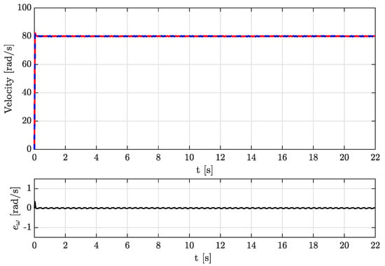
Figure 2.
Simulation results, test 1: estimated velocity () vs. velocity (−) and the velocity estimation error (−).

Figure 3.
Simulation results, test 1: estimated load torque () vs. load toque (−) and the load torque estimation error (−).
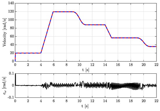
Figure 4.
Simulation results, test 2: estimated velocity () vs. velocity (−) and the velocity estimation error (−).

Figure 5.
Simulation results, test 2: estimated load torque () vs. load toque (−) and the load torque estimation error (−).
Table 2 displays the RMSE values obtained in the two tests. The error between the estimated load torque and the actual load torque is attributed to the sampling period with which the observer is executed, as well as to the noise present in the currents. How these two factors impact the estimation of the states is analyzed in [17]. However, even in the presence of noise, the observer reconstructs the states and the load torque with a small error.

Table 2.
RMS error values.
5. Experimental Results
In this section, the experimental validation of the proposed estimator is presented. First, the experimental platform used is described, as well as the algorithm employed to calculate the angular position from the information provided by the Hall effect sensors. Lastly, the experimental results are presented and analyzed.
5.1. Experimental Test Bench
The brushless DC motor utilized in this study was the BLY344S-240V-3000 model from Anaheim Automation (Anaheim, CA, USA). Detailed parameters extracted from the datasheet and experiments can be found in Table 1. This BLDC motor is equipped with three Hall effect sensors positioned at 120 electrical degrees apart on the rear side of the motor. The Hall effect sensors work with additional magnets mounted on the rotor shaft. These sensors are essential for a rough calculation of position and speed and are commonly used to ensure the correct commutation of the motor phases during each transition of these sensors, which occurs every 60 electrical degrees.
Furthermore, the absolute capacitive encoder AMT333S-V from CUI Devices (Tualatin, OR, USA), which offers configurable resolution ranging from 48 to 4096 pulses per revolution, was attached to the motor shaft. This encoder was used to calculate the rotor’s speed and compare it with the speed estimated by the proposed observer. In this case, the encoder was configured with a resolution of 2000 PPR.
The inverter employed for this setup was the high-voltage digital motor control and power factor correction kit (TMDSHVMTRPFCKIT) from Texas Instruments (TI) (Dallas, TX, USA). This board includes a 3-phase inverter stage designed to control motors with voltages up to 450 [V] DC, and an AC rectifier stage for generating the DC bus voltage required by the inverter, and it is compatible with a wide variety of Texas Instruments microcontroller cards. The current measurement was carried out on the low side of the inverter using shunt resistors for each stator phase.
The control card used was based on the F28379D Delfino microcontroller also from TI, which is a 32-bit floating-point microcontroller unit with dual CPUs optimized for real-time control applications. Similar to the simulation, the method employed for motor control was field-oriented control. The gains of the speed PI controller were tuned, taking into consideration all the devices coupled to the BLDC motor. This was done with the aim of minimizing the impact of the load torque on speed tracking, as the main objective was to demonstrate the operation of the observer. The sampling time at which the cascade observer and current control were executed was the same as in the simulations, namely [ms]. A direct current motor was employed, connected to the shaft of the BLDC motor as a variable load torque. This was achieved by following a current trajectory that generated a load torque similar to that in the simulations. To measure the torque generated by this motor, the FSH01996 torque sensor from Futek was mounted between the DC motor and the BLDC motor. This sensor can measure up to 5 Nm of load torque and was used to compare the estimated torque from the observer with the measured value of the sensor. Figure 6 provides an illustration of the experimental setup.

Figure 6.
Experimental test bench.
5.2. Position Estimation Algorithm-PEA
While it is possible to use an encoder to obtain angular position, it was decided to utilize Hall effect sensor signals for this purpose, as BLDC motors typically come equipped with them. However, it should be noted that three Hall effect sensors only provide new information at intervals of electrical degrees, whereas the proposed observer requires continuous measurement of angular position. To address this limitation, a position estimation algorithm (PEA) was developed, making use of the state of the Hall effect sensors and the elapsed time between transitions.
In summary, the PEA operates as a saturated integrator with a variable initial condition. The integrator takes the speed estimate, , where , and represents the time elapsed between transitions of the Hall effect sensors, as its input. Whenever one of these transitions occurs, the integrator is reset, and a new initial condition is determined. The initial condition of the integrator depends on the current state of the Hall effect sensors and the rotation sequence. Figure 7 illustrates the relationship between the state of the Hall effect sensors and the position for a constant speed motion, where 0 and 1 in the upper right part of the figure indicate whether a given Hall effect sensor is active or not. The numbers 5, 4, 2, 6, 3, 1 at the bottom show the switching state considering the three Hall effect sensors, related to the electrical angular position indicated on the right that goes from 0 to , and Figure 8 shows a simple diagram of the position estimation algorithm.

Figure 7.
Relationship between Hall sensor signals and wrapped position (−). With Hall effect sensor signal A (−), Hall effect sensor signal B (−) and Hall effect sensor signal C (−).

Figure 8.
Position estimation algorithm block diagram.
5.3. Disturbance Estimation
Similar to the simulations, two experiments were conducted on the platform. One involved maintaining a constant speed with a variable load torque, where the load torque applied to the BLDC motor was controlled using the DC motor current control. In the second experiment, both speed and load torque varied over time. The estimator gains used in these tests were the same as those used in the simulations. Figure 9 shows the electrical position calculated with PEA and the measured position with the encoder.

Figure 9.
Experimental results with flywheel: estimated electrical position with PEA () vs. encoder position (−).
In the first test the speed reference was the same as in the first simulation, that is, constant speed and time-varying load torque. Figure 10 illustrates the behavior of the estimated angular velocity ,the measured velocity , and the velocity estimation error , with Figure 11 showing the estimated load torque , the measured load torque and the load torque estimation error .
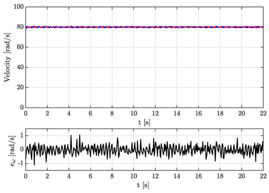
Figure 10.
Experimental results, test 1: estimated velocity () vs. measured velocity (−) and the velocity estimation error (−).
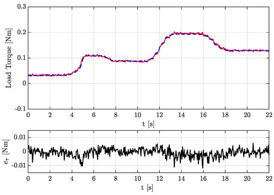
Figure 11.
Experimental results, test 1: estimated load torque () vs. measured load toque (−) and the load torque estimation error (−).
In the second test, the speed reference and the load torquewere both time-varying, similar to the second simulation. Figure 12 illustrates the behavior of the estimated angular velocity compared with the measured velocity and the velocity estimation error . Figure 13 depicts the estimated load torque , the measured load torque , and the load torque estimation error .
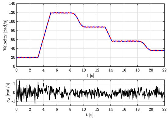
Figure 12.
Experimental results, test 2: estimated velocity () vs. measured velocity (−) and the velocity estimation error (−).

Figure 13.
Experimental results, test 2: estimated load torque () vs. measured load toque (−) and the load torque estimation error (−).
5.4. Results Discussion
Comparing the experimental results with the numerical simulations, it is clear to see that the signals are much noisier than in the simulations; however, the RMS errors displayed in Table 3 are relatively small despite this in both tests. The size of the RMS velocity estimation error is the most affected and it is clearly influenced by the inclusion in the experiments of the PEA, that was not used in the simulations; the size of the RMS torque estimation error was also impacted by noise, although the increase on the error size was modest in this case.

Table 3.
RMS error values.
The effect of obtaining the position through the PEA, which relies on Hall effect sensors, in the estimation of the angular velocity is larger at low velocities. This is evident in Figure 14, which illustrates the relative velocity estimation error across a wide range of velocities. This relative error remains below 2% for velocities exceeding . In contrast, Figure 15 displays the relative velocity estimation error using the position obtained through the encoder mounted on the platform, rather than the one obtained through the PEA. It is clear to see that the estimation error remains small even at low speeds. Therefore, the suggested cascade observer, when utilizing the PEA, can effectively estimate torque and velocity within a range of medium to high velocities, and for low-velocity applications, it is recommended to use an encoder in conjunction with the proposed observer.

Figure 14.
Relative estimation error with respect to angular velocity using Hall effect sensors.

Figure 15.
Relative estimation error with respect to angular velocity using encoder.
6. Conclusions
A load torque observer for a BLDC motor was proposed in this article. It was demonstrated through simulations and experiments that the observer can estimate the load torque and velocity with relatively small errors, under the reasonable assumption that the variable torque and its time derivatives are bounded, even in the presence of noise in the current measurements. In addition to this, it was possible to estimate the state variables and the load torque. For medium to high speeds it is possible to use the position information from the Hall effect sensors, that are typically mounted on these type of motors. For low speeds, the inclusion of an encoder is recommended. In all cases, the use of expensive torque sensors for high-performance control applications can be avoided.
Author Contributions
Formal analysis A.C.-A., A.d.l.G. and L.A.-I. Investigation A.C.-A. Funding acquisition L.A.-I. Supervision A.d.l.G. and L.A.-I. Software A.C.-A. Writing—original draft preparation A.C.-A. and A.d.l.G. Writing—review & editing L.A.-I. All authors have read and agreed to the published version of the manuscript.
Funding
This research was funded by PAPIIT grant number IT101420.
Data Availability Statement
The data that support the findings of this study are available from the authors, upon reasonable request.
Conflicts of Interest
The authors declare no conflict of interest.
References
- Ehsani, M.; Gao, Y.; Longo, S.; Ebrahim, K. Modern Electric, Hybrid Electric, and Fuel Cell, Vehicles; CRC Press: Boca Raton, FL, USA, 2018. [Google Scholar]
- Zarma, T.J.; Galadima, A.A.; Aminu, M.A. Review of Motors for Electrical Vehicles. J. Sci. Res. Rep. 2019, 24, 1–6. [Google Scholar] [CrossRef]
- Yang, S.-C.; Lorenz, R.D. Surface Permanent-Magnet Machine Self-Sensing at Zero and Low Speeds Using Improved Observer for Position, Velocity, and Disturbance Torque Estimation. IEEE Trans. Ind. Appl. 2012, 48, 151–160. [Google Scholar] [CrossRef]
- Liao, Z.; Liu, Z.; Chen, L.; Lyu, M.; Wang, Z.; Wang, D.; Wu, F.; Wei, H. An Integrated Observer Framework Based Mechanical Parameters Identification for Adaptive Control of Permanent Magnet Synchronous Motor. TUP Complex Syst. Model. Simul. 2022, 2, 354–367. [Google Scholar] [CrossRef]
- Wang, L.; Tang, Z.; Zhang, P.; Liu, X.; Wang, D.; Li, X. Double Extended Sliding Mode Observer-Based Synchronous Estimation of Total Inertia and Load Torque for PMSM-Driven Spindle-Tool Systems. IEEE Trans. Ind. Inform. 2022, 19, 8496–8507. [Google Scholar] [CrossRef]
- Yang, C.; Song, B.; Xie, Y.; Zheng, S.; Tang, X. Adaptive Identification of Nonlinear Friction and Load Torque for PMSM Drives via a Parallel-Observer-Based Network with Model Compensation. IEEE Trans. Power Electron. 2023, 38, 5875–5897. [Google Scholar] [CrossRef]
- de la Guerra, A.; Alvarez–Icaza, L.; Torres, L. Brushless DC Motor Control with Unknown and Variable Torque Load. Elsevier IFAC-PapersOnLine 2018, 51, 644–649. [Google Scholar] [CrossRef]
- de la Guerra, A.; Alvarez-Icaza, L. Robust Control of the Brushless DC Motor with Variable Torque Load for Automotive Applications. Electr. Power Compon. Syst. 2020, 48, 117–127. [Google Scholar] [CrossRef]
- Quattrocchi, G.; Iacono, A.; Berri, P.C.; Dalla Vedova, M.D.; Maggiore, P. A new method for friction estimation in EMA transmissions. Actuators 2021, 10, 194. [Google Scholar] [CrossRef]
- Kerem, A. Torque estimation of electric vehicle motor using adaptive-network based fuzzy inference systems. Murat CINIVIZ Int. J. Automot. Eng. Technol. 2021, 10, 33–41. [Google Scholar] [CrossRef]
- Nair, D.S.; Jagadanand, G.; George, S. Torque estimation using Kalman filter and extended Kalman filter algorithms for a sensorless direct torque controlled BLDC motor drive: A comparative study. J. Electr. Eng. Technol. 2021, 16, 2621–2634. [Google Scholar] [CrossRef]
- Sikora, A.; Zielonka, A.; Woźniak, M. Minimization of energy losses in the BLDC motor for improved control and power supply of the system under Static Load. Sensors 2022, 22, 1058. [Google Scholar] [CrossRef] [PubMed]
- Yoo, A.; Sul, S.-K.; Lee, D.-C.; Jun, C.-S. Novel Speed and Rotor Position Estimation Strategy Using a Dual Observer for Low-Resolution Position Sensors. IEEE Trans. Power Electron. 2009, 24, 2897–2906. [Google Scholar] [CrossRef]
- Ahn, H.-J.; Lee, D.-M. A new bumpless rotor-flux position estimation scheme for vector-controlled washing machine. IEEE Trans. Ind. Inform. 2016, 12, 466–473. [Google Scholar] [CrossRef]
- Park, J.S.; Lee, K.-D. Online advanced angle adjustment method for sinusoidal BLDC motors with misaligned hall sensors. IEEE Trans. Power Electron. 2017, 32, 8247–8253. [Google Scholar] [CrossRef]
- Kolano, K.; Drzymała, B.; Gęca, J. Sinusoidal Control of a Brushless DC Motor with Misalignment of Hall Sensors. Energies 2021, 14, 3845. [Google Scholar] [CrossRef]
- Fridman, L.; Levant, A.; Davila, J. Observation of linear systems with unknown inputs via high-order sliding-modes. Int. J. Syst. Sci. 2007, 38, 773–791. [Google Scholar] [CrossRef]
- Moreno, J. Existence of unknown input observers and feedback passivity for linear systems. In Proceedings of the 40th IEEE Conference on Decision and Control, Orlando, FL, USA, 4–7 December 2001; pp. 3366–3371. [Google Scholar]
- Chiasson, J.N. Modeling and High Performance Control of Electric Machines; John Wiley & Sons: Hoboken, NJ, USA, 2005. [Google Scholar]
- Hautus, M.L.J. Strong detectability and observers. Linear Algebra Its Appl. 1983, 50, 353–368. [Google Scholar] [CrossRef]
- Isidori, A. Global almost disturbance decoupling with stability for non minimum-phase single-input single-output nonlinear systems. Syst. Control. Lett. 1996, 28, 115–122. [Google Scholar] [CrossRef]
Disclaimer/Publisher’s Note: The statements, opinions and data contained in all publications are solely those of the individual author(s) and contributor(s) and not of MDPI and/or the editor(s). MDPI and/or the editor(s) disclaim responsibility for any injury to people or property resulting from any ideas, methods, instructions or products referred to in the content. |
© 2023 by the authors. Licensee MDPI, Basel, Switzerland. This article is an open access article distributed under the terms and conditions of the Creative Commons Attribution (CC BY) license (https://creativecommons.org/licenses/by/4.0/).