Figure 1.
Top view of the NASA Maxwell X-57 distributed propulsion aircraft [
19].
Figure 1.
Top view of the NASA Maxwell X-57 distributed propulsion aircraft [
19].
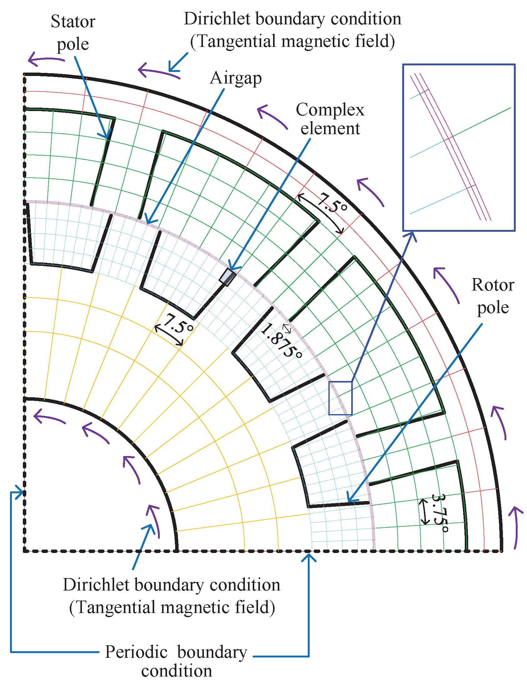
Figure 2.
An example reluctance mesh for 12/16 SRM [
18].
Figure 2.
An example reluctance mesh for 12/16 SRM [
18].
Figure 3.
Structure of a reluctance mesh element and MMF source arrangement.
Figure 3.
Structure of a reluctance mesh element and MMF source arrangement.
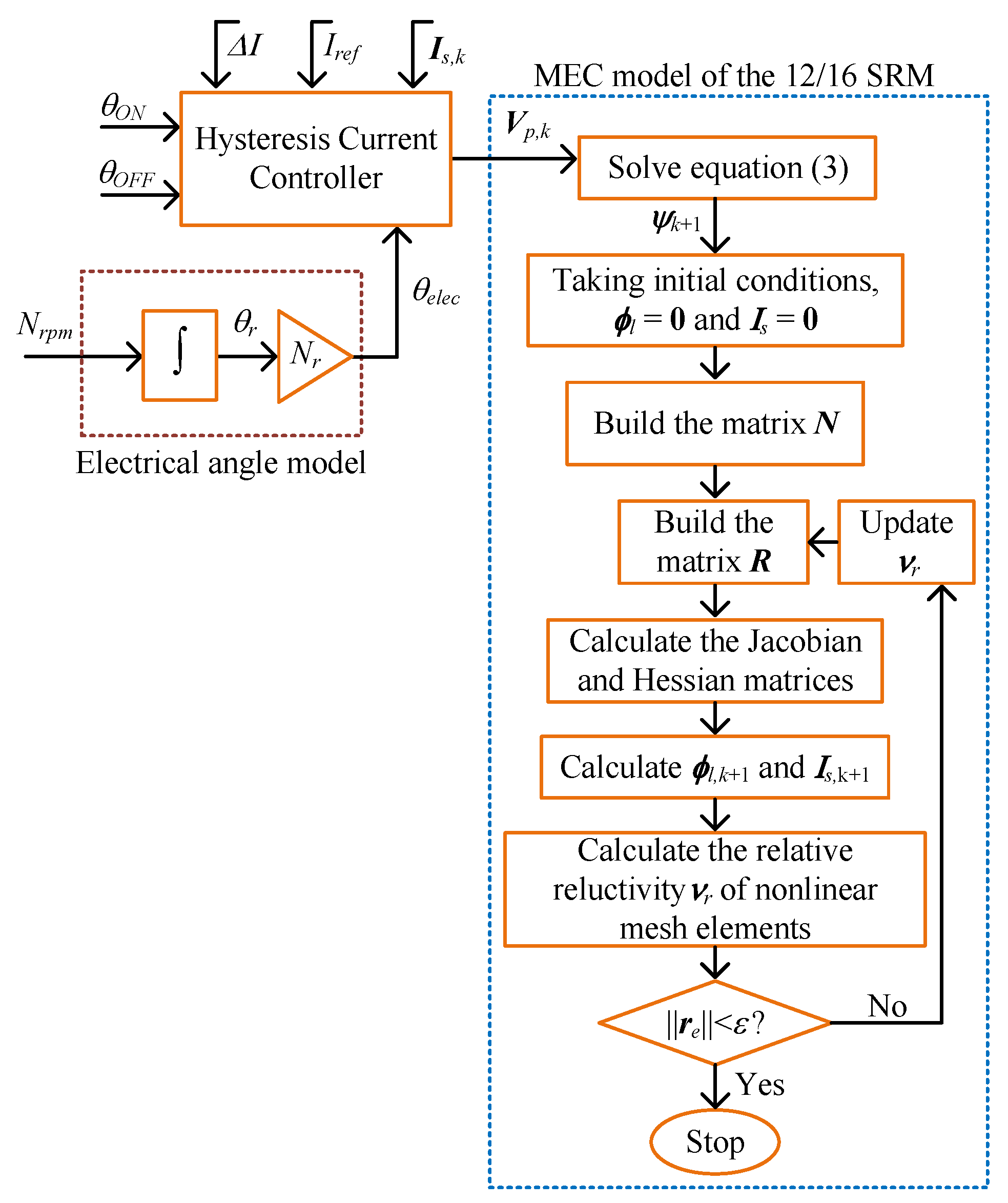
Figure 4.
The procedure for implementing the dynamic model, including the magnetic saturation effects and mutual coupling.
Figure 4.
The procedure for implementing the dynamic model, including the magnetic saturation effects and mutual coupling.
Figure 5.
Static electromagnetic torque at a 60 A excitation current for 6/16, 12/16, and 24/16 SRMs.
Figure 5.
Static electromagnetic torque at a 60 A excitation current for 6/16, 12/16, and 24/16 SRMs.
Figure 6.
Static electromagnetic torque at a 60 A excitation current for 12/8, 12/16, and 12/20 SRMs.
Figure 6.
Static electromagnetic torque at a 60 A excitation current for 12/8, 12/16, and 12/20 SRMs.
Figure 7.
Main geometry parameters of the 12/16 SRM.
Figure 7.
Main geometry parameters of the 12/16 SRM.
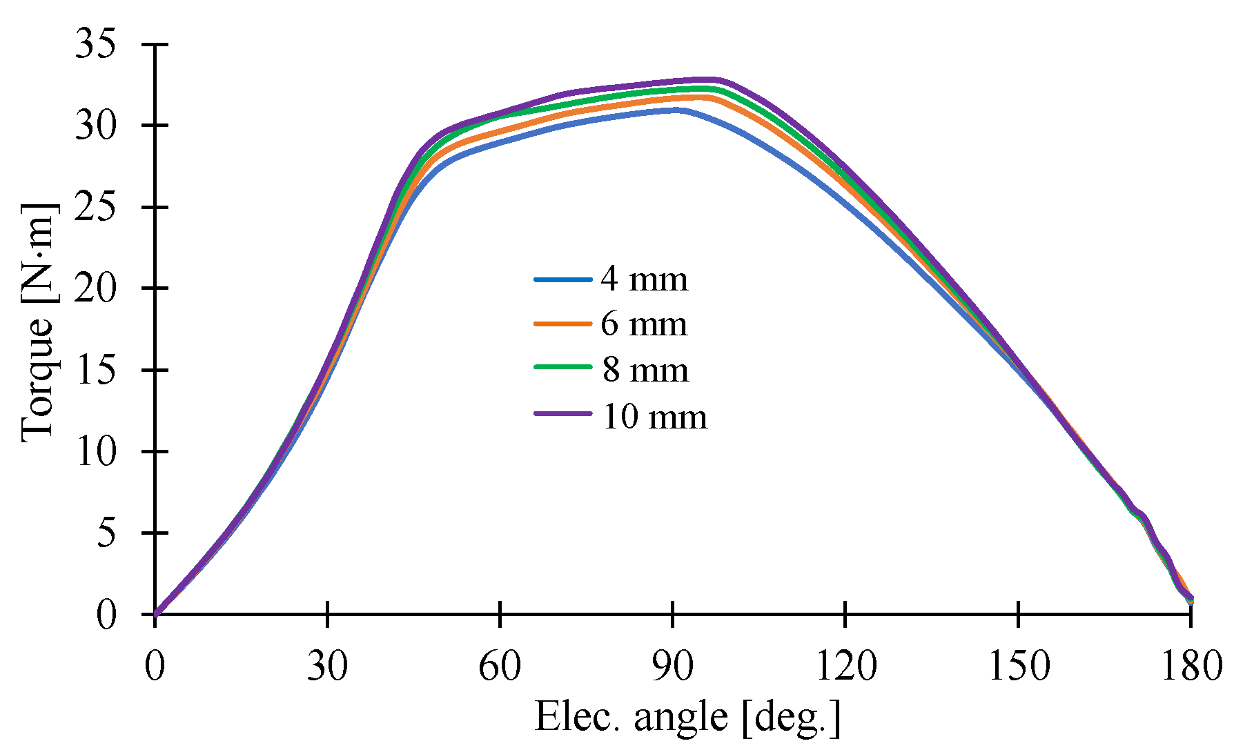
Figure 8.
Dynamic electromagnetic torque from the MEC model at 5450 r/min at different airgaps.
Figure 8.
Dynamic electromagnetic torque from the MEC model at 5450 r/min at different airgaps.
Figure 9.
Static torque profiles at a 60 A excitation current for different rotor pole heights.
Figure 9.
Static torque profiles at a 60 A excitation current for different rotor pole heights.
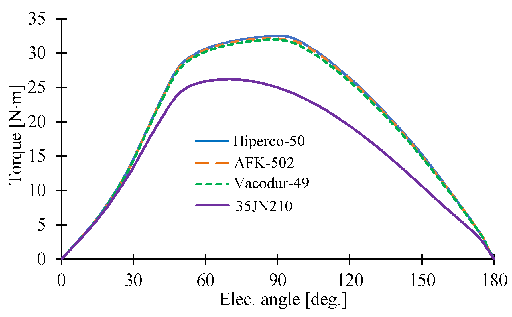
Figure 10.
Static torque profiles at a 60 A excitation current for different magnetic materials.
Figure 10.
Static torque profiles at a 60 A excitation current for different magnetic materials.
Figure 11.
Characteristics of Hiperco-50 0.15 mm laminations: (a) BH characteristics and (b) specific core losses.
Figure 11.
Characteristics of Hiperco-50 0.15 mm laminations: (a) BH characteristics and (b) specific core losses.
Figure 12.
The steady-state temperature of the motor computed in MotorCAD.
Figure 12.
The steady-state temperature of the motor computed in MotorCAD.
Figure 13.
The temperature variation in the hotspot during winding under peak operating conditions.
Figure 13.
The temperature variation in the hotspot during winding under peak operating conditions.
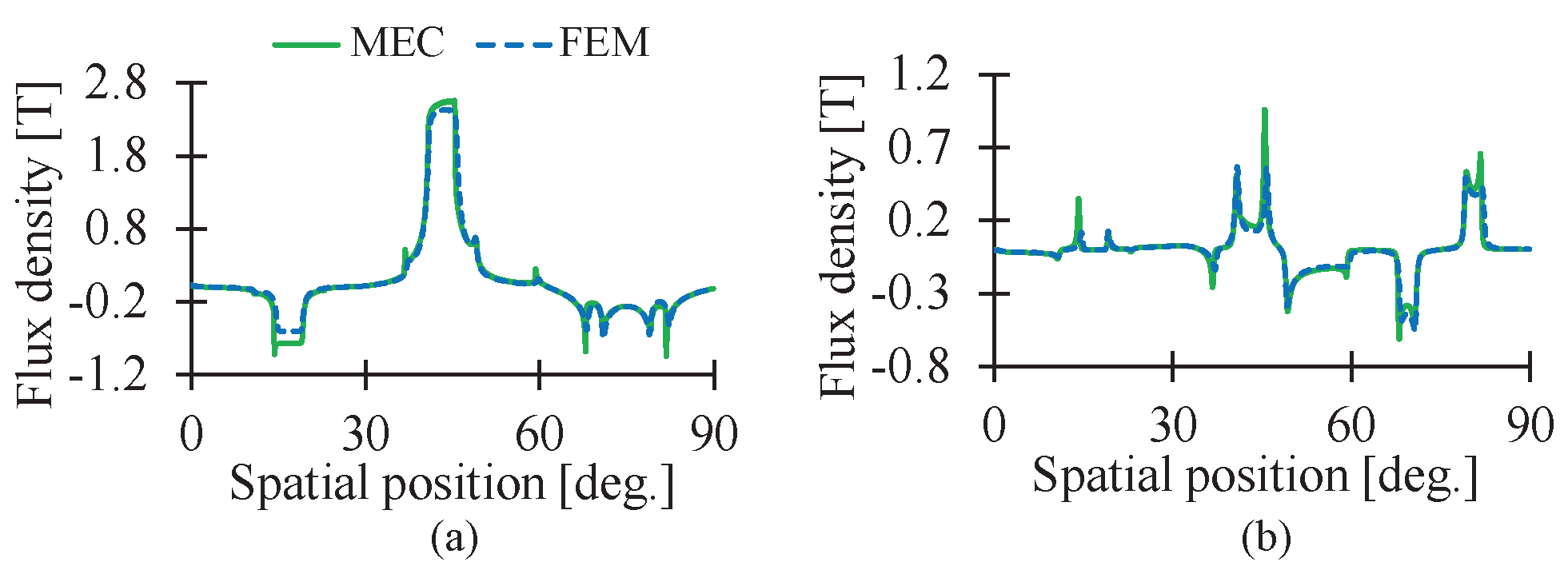
Figure 14.
Airgap flux density waveforms at 60 A static excitation current: (a) radial flux density at the unaligned position, (b) tangential flux density at the unaligned position, (c) radial flux density at the aligned position, and (d) tangential flux density at the aligned position.
Figure 14.
Airgap flux density waveforms at 60 A static excitation current: (a) radial flux density at the unaligned position, (b) tangential flux density at the unaligned position, (c) radial flux density at the aligned position, and (d) tangential flux density at the aligned position.
Figure 15.
Magnetic flux density contours at 60 A static excitation current: (a) unaligned position, MEC, (b) unaligned position, FEM, (c) aligned position, MEC, and (d) aligned position, FEM.
Figure 15.
Magnetic flux density contours at 60 A static excitation current: (a) unaligned position, MEC, (b) unaligned position, FEM, (c) aligned position, MEC, and (d) aligned position, FEM.
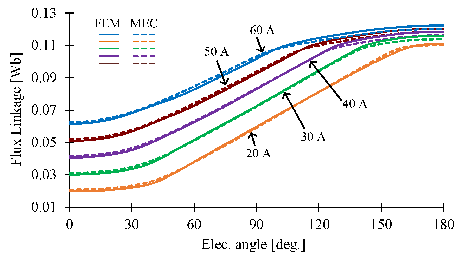
Figure 16.
Static phase flux linkage characteristics at different currents.
Figure 16.
Static phase flux linkage characteristics at different currents.
Figure 17.
Static phase voltage characteristics at 5450 r/min at different currents.
Figure 17.
Static phase voltage characteristics at 5450 r/min at different currents.
Figure 18.
Static torque characteristics at different currents.
Figure 18.
Static torque characteristics at different currents.
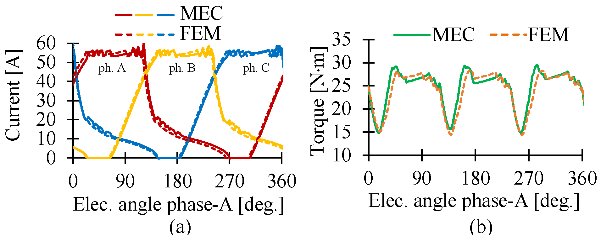
Figure 19.
Dynamic characteristics at 2000 r/min at 385 V DC: (a) phase currents A, , and and (b) developed electromagnetic torque.
Figure 19.
Dynamic characteristics at 2000 r/min at 385 V DC: (a) phase currents A, , and and (b) developed electromagnetic torque.
Figure 20.
Dynamic characteristics at 4000 r/min at 385 V DC: (a) phase currents A, , and and (b) developed electromagnetic torque.
Figure 20.
Dynamic characteristics at 4000 r/min at 385 V DC: (a) phase currents A, , and and (b) developed electromagnetic torque.
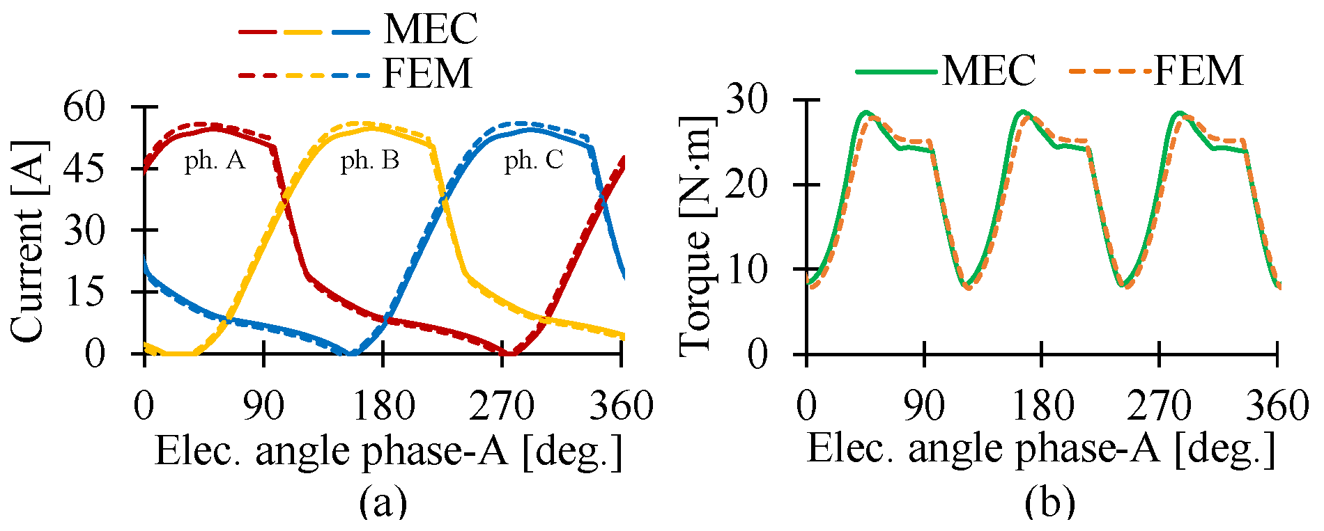
Figure 21.
Dynamic characteristics at 5450 r/min at 385 V DC: (a) phase currents A, , and and (b) developed electromagnetic torque.
Figure 21.
Dynamic characteristics at 5450 r/min at 385 V DC: (a) phase currents A, , and and (b) developed electromagnetic torque.
Figure 22.
Dynamic characteristics at 5460 r/min at 385 V DC: (a) phase currents A, , and and (b) developed electromagnetic torque.
Figure 22.
Dynamic characteristics at 5460 r/min at 385 V DC: (a) phase currents A, , and and (b) developed electromagnetic torque.
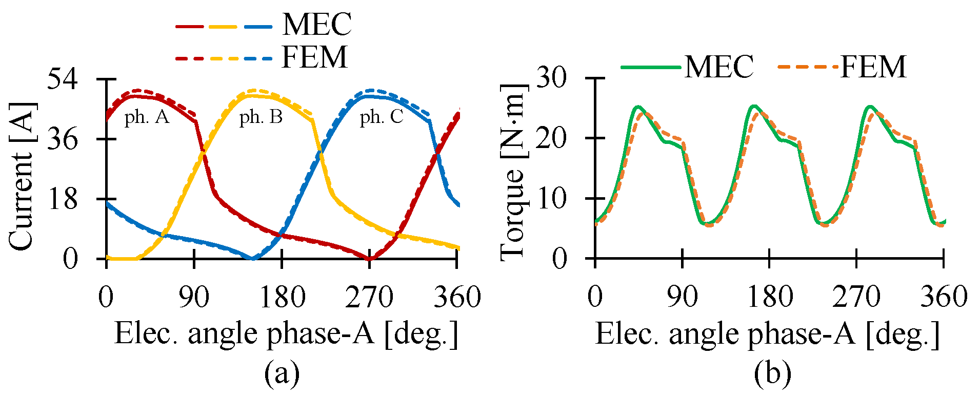
Figure 23.
Dynamic characteristics at 7000 r/min at 385 V DC: (a) phase currents A, , and and (b) developed electromagnetic torque.
Figure 23.
Dynamic characteristics at 7000 r/min at 385 V DC: (a) phase currents A, , and and (b) developed electromagnetic torque.
Figure 24.
Dynamic characteristics at 8000 r/min at 385 V DC: (a) phase currents A, , and and (b) developed electromagnetic torque.
Figure 24.
Dynamic characteristics at 8000 r/min at 385 V DC: (a) phase currents A, , and and (b) developed electromagnetic torque.
Figure 25.
Airgap flux density at
for phase currents in
Figure 21: (a) radial component and (b) tangential component.
Figure 25.
Airgap flux density at
for phase currents in
Figure 21: (a) radial component and (b) tangential component.
Figure 26.
Magnetic flux density contours at
for the current waveform in
Figure 21.
Figure 26.
Magnetic flux density contours at
for the current waveform in
Figure 21.
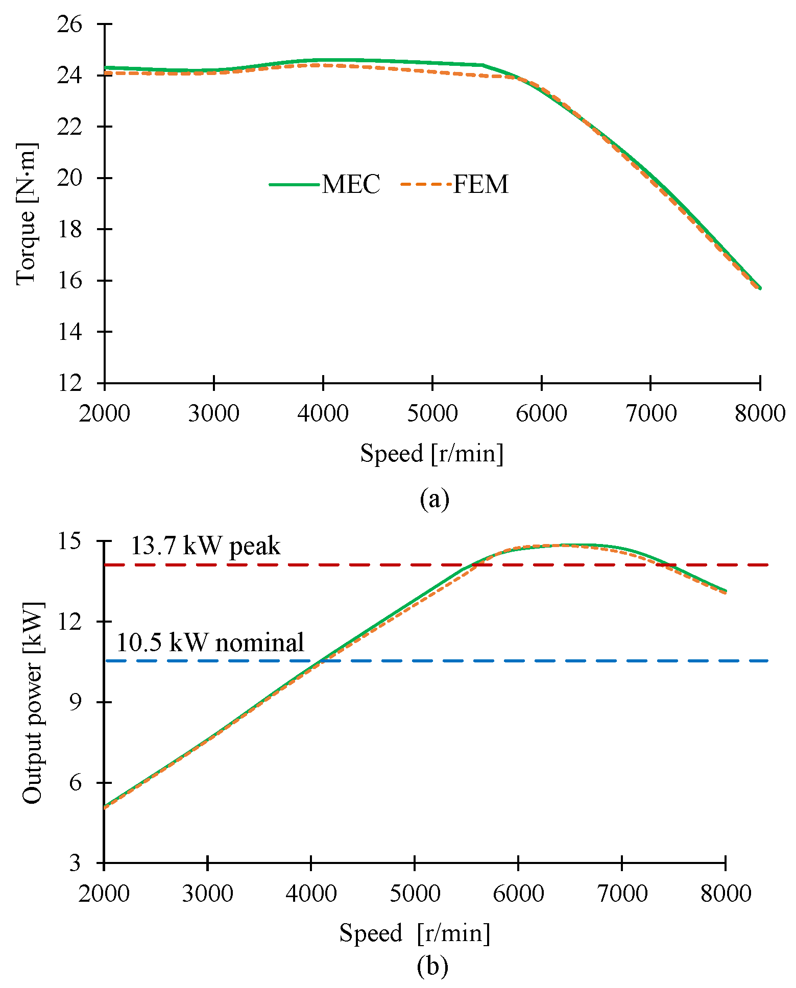
Figure 27.
Motor characteristics for the peak operating point of the 12/16 SRM at 385 V DC link voltage: (a) torque–speed characteristics and (b) power–speed characteristics.
Figure 27.
Motor characteristics for the peak operating point of the 12/16 SRM at 385 V DC link voltage: (a) torque–speed characteristics and (b) power–speed characteristics.
Table 1.
Main design specifications of an HLM.
Table 1.
Main design specifications of an HLM.
| Electromagnetic Design Parameters |
|---|
| Peak output power | 13.7 kW |
| Peak torque | 24 N·m |
| Minimum torque density | 18.8 N·m/L |
| Base speed | 5450 r/min |
| RMS phase current | 35 A |
| DC link voltage | 385–538 V |
| Number of phases | 3 |
| Geometry Constraints |
| Maximum motor diameter (with casing) | 161.5 mm |
| Maximum stator outer diameter (without casing) | 156.45 mm |
| Maximum stator axial length including end turns | 66.4 mm |
| Expected Performance |
| 1. Provide 24 N·m of torque between 2000 and 5450 r/min and 22 N·m of torque at 5460 r/min. |
| 2. Capable of producing 10.5 kW output power at 5460 r/min and at 460 V DC link voltage with a minimum efficiency of 93%. |
Table 2.
Fill factor and current density constraints.
Table 2.
Fill factor and current density constraints.
| Characteristic | Maximum Allowable Value | Achieved by PMSM Design |
|---|
| Wire fill factor | 60% | 58.4% |
| Current density | 11 A/mm2 | 10.7 A/mm2 |
Table 3.
Average torque and torque ripple of the torque profiles in
Figure 8.
Table 3.
Average torque and torque ripple of the torque profiles in
Figure 8.
| Airgap Length | Avg. Torque | Pk–Pk Torque Ripple | Torque Density |
|---|
| 0.4 mm | 23.6 N·m | 14 N·m | 18.5 N·m/L |
| 0.35 mm | 24.6 N·m | 14.59 N·m | 19.3 N·m/L |
| 0.3 mm | 25.5 N·m | 15.23 N·m | 20 N·m/L |
Table 4.
Proposed dimensions of the SRM geometry.
Table 4.
Proposed dimensions of the SRM geometry.
| Parameter | Value |
|---|
| Outer diameter () | 156.45 mm |
| Bore diameter () | 115 mm |
| Shaft diameter () | 50 mm |
| Airgap length (g) | 0.35 mm |
| Stator pole arc angle () | 8.2∘ |
| Rotor pole arc angle () | 8.5∘ |
| Stator pole height () | 15 mm |
| Rotor pole height () | 10 mm |
| Stator back-iron thickness () | 5.725 mm |
| Rotor back-iron thickness () | 22.15 mm |
Table 5.
Magnetic, thermal, and mechanical characteristics of the cobalt–iron materials [
23,
24,
25].
Table 5.
Magnetic, thermal, and mechanical characteristics of the cobalt–iron materials [
23,
24,
25].
| Characteristic | Hiperco-50 | AFK-502 | Vacodur-49 |
|---|
| Specific core loss | 400 Hz/2 T | 56.7 W/kg | 70 W/kg | 60 W/kg |
| 1000 Hz/2 T | 301 W/kg | 320 W/kg | 330 W/kg |
| Saturation flux density | 2.3 T | 2.32 T | 2.3 T |
| Resistivity | 0.4 | 0.4 | 0.42 |
| Yield strength | 331 MPa–414 Mpa | 300 MPa–420 Mpa | 210 MPa–390 Mpa |
| Thermal conductivity | 29.8 W/m·K | 32 W/m·K | 32 W/m·K |
Table 6.
Proposed winding configuration and axial length constraints.
Table 6.
Proposed winding configuration and axial length constraints.
| Parameter | Value |
|---|
| Number of turns per coil () | 32 |
| Number of strands | 3 |
| Wire fill factor | 58.4% |
| Maximum current density | 10.96 A/mm2 |
| Wire gauge | 17 AWG heavy-build |
| Coil resistance () | 0.02768 |
| Stator core stack length () | 47 mm |
| Estimated stacking factor | 97% |
| Estimated end turn length () | 9.7 mm |
| Total axial length () | 66.4 mm |
Table 7.
Comparison of the SRM design with benchmark PMSM design.
Table 7.
Comparison of the SRM design with benchmark PMSM design.
| Design Parameters | SRM Design | PMSM Design |
|---|
| Outer diameter | 156.45 mm | 156.45 mm |
| Axial length | 66.4 mm | 51.5 mm |
| Torque density | 19.3 Nm/L | 24.2 Nm/L |
| Current density | 10.96 A/mm2 (<11 A/mm2) | 10.7 A/mm2 (<11 A/mm2) |
| Fill factor | 58.4% (<60%) | 58.4% (<60%) |
| Efficiency | 95.46% | 96% |
Table 8.
Thermal conductivities of materials used in the thermal analysis.
Table 8.
Thermal conductivities of materials used in the thermal analysis.
| Component | Material | Thermal Conductivity |
|---|
| Housing (heatsink) | Aluminum 2024-T3 | 120 W/m2 |
| Stator and rotor | Hiperco-50 | 20 W/m2 |
| Windings | Copper | 400 W/m2 |
| Stator slot voids | Epoxy resin | 1 W/m2 |
| Slot linear | Nomex 410 | 0.14 W/m2 |
Table 9.
Flux density comparison at points P
1, P
2, and P
3 in
Figure 15 in static simulations.
Table 9.
Flux density comparison at points P
1, P
2, and P
3 in
Figure 15 in static simulations.
| Position | Point P1 | Point P2 | Point P3 |
|---|
| MEC | FEM | % Error | MEC | FEM | % Error | MEC | FEM | % Error |
|---|
| Unaligned | 0.98 T | 0.96 T | 2.1% | 1.43 T | 1.31 T | 9.1% | 0.55 T | 0.54 T | 1.9% |
| Aligned | 1.89 T | 1.8 T | 5% | 2.41 T | 2.33 T | 3.4% | 2.31 T | 2.25 T | 2.7% |
Table 10.
Comparison of RMS current, average torque, and peak–peak torque ripple from the MEC and FEM models.
Table 10.
Comparison of RMS current, average torque, and peak–peak torque ripple from the MEC and FEM models.
| Speed | RMS Current | Avg. Torque | Pk–Pk Torque Ripple |
|---|
| MEC | FEM | % Error | MEC | FEM | % Error | MEC | FEM | % Error |
|---|
| 2000 r/min | 35.8 A | 34.9 A | 3.2% | 24.2 N·m | 25.3 N·m | 4.3% | 11.7 N·m | 8.7 N·m | 25.6% |
| 4000 r/min | 35.5 A | 34.8 A | 2% | 24.5 N·m | 24.4 N·m | 0.6% | 7.86 N·m | 10.37 N·m | 9.7% |
| 5450 r/min | 34.3 A | 34.2 A | 0.3% | 24.4 N·m | 24 N·m | 2.5% | 14.59 N·m | 13.97 N·m | 4.44% |
| 5460 r/min | 34 A | 34.1 A | 0.3% | 24.4 N·m | 24 N·m | 2.5% | 14.86 N·m | 14.18 N·m | 4.8% |
| 6000 r/min | 32 A | 33. 6A | 4.8% | 23.4 N·m | 23.5 N·m | 0.4% | 15.95 N·m | 14.89 N·m | 7.12% |
| 7000 r/min | 31.7 A | 32.5 A | 2.5% | 20.1 N·m | 19.9 N·m | 1% | 20.45 N·m | 20.13 N·m | 1.59% |
| 8000 r/min | 27.8 A | 28.6 A | 2.8% | 15.7 N·m | 15.6 N·m | 0.6% | 19.5 N·m | 18.72 N·m | 4.17% |
Table 11.
Flux density comparison at points P
1, P
2, P
3, P
4, P
5, and P
6 for the dynamic operation in
Figure 26.
Table 11.
Flux density comparison at points P
1, P
2, P
3, P
4, P
5, and P
6 for the dynamic operation in
Figure 26.
| Location | MEC | FEM | % Error |
|---|
| Point P1 | 1.01 T | 0.89 T | 13.5% |
| Point P2 | 0.39 T | 0.38 T | 2.6% |
| Point P3 | 2.24 T | 2.26 T | 0.9% |
| Point P4 | 2.03 T | 1.98 T | 2.5% |
| Point P5 | 0.61 T | 0.52 T | 17.3% |
| Point P6 | 0.63 T | 0.54 T | 16.7% |


