Kinematic Calibration Method for Large-Sized 7-DoF Hybrid Spray-Painting Robots

Abstract

Large-sized seven-degrees-of-freedom (7-DoF) hybrid spray-painting robots combine ample working space and high flexibility, making them lucrative for the spray painting of aircraft and rocket surfaces. However, their kinematic calibration is hindered by gravitational deformation, which problem is addressed in this study by introducing a rigid-flexible coupling error modeling method. The latter combines the finite element method (FEM) and stiffness matrix method to assess the spatial gravitational deformation of a hybrid robot, which is then introduced into a geometric error model to establish the rigid-flexible coupling error identification model. Given many redundant parameters in the identification model for 7-DoF robots, these parameters are classified and simplified using the nonlinear least-square regularization method for parameter identification. Combining the inverse solution of 7-DoF spray-painting robots with dynamic characteristics considered, an error compensation method for 7-DoF robots is proposed. The kinematic calibration test results strongly indicate that position errors are significantly reduced with gravity compensation taken into consideration, and error convergence speed increases, demonstrating that the kinematic calibration method is feasible and can effectively improve the accuracy of spray-painting robots. The mean errors in the X- and Y-directions are reduced by 20 and 17%, respectively, compared to the conventional method. The proposed method is instrumental in the accurate kinematic calibration of large-sized 7-DoF hybrid robots.

1. Introduction

With the rapid development of aviation and spacecraft industries, large-sized aero- and spacecraft production is gradually increasing. Their surface is usually protected from erosion and heat by special coatings [1], with thickness and uniformity satisfying stringent requirements [2]. Compared to manual operation, robot spray painting is more stable, high-efficient, and uniform, and thus has a higher coating quality, making automated painting a vital development direction [3,4]. With the advantages of good dynamic characteristics, increased flexibility, high acceleration, ample working space, and the ability to keep the spray gun perpendicular to the painted surface and avoid obstacles, a hybrid robot with seven degrees of freedom (7-DoF) [5,6] is a lucrative choice for the spray painting of large-sized airplanes and rockets.

However, in practice, the accuracy of spray painting by 7-DoF hybrid robots is significantly deteriorated by the following factors:

(1) The robot has many joints, which may have relatively large errors in manufacturing and assembly, and the significant geometric errors can result in a relatively low absolute position accuracy [7,8].

(2) Due to the large size of the robot, which can extend up to 4 m, gravitational deformation significantly impacts the accuracy of this mechanism.

Thus, improving the kinematic accuracy of this mechanism becomes a problem to be solved. The accuracy problem limits the operational capability of the spray-painting robot and makes it challenging to perform spray-painting tasks with a demanding requirement for accuracy. Therefore, improving the absolute kinematic accuracy of the spray-painting robots is of great significance.

Generally, the above problem can be mitigated by kinematic calibration [9,10]. However, for the proposed 7-DoF hybrid spray-painting robot, conventional kinematic calibration, which considers only geometric errors in error modeling, is hardly sufficient because gravitational deformation also significantly impacts the terminal position error of the proposed large-sized robot with a cantilever-like terminal telescopic mechanism. The above gravitational deformation’s effect on the terminal error leads to inaccurate terminal posture error modeling.

This paper attempts to solve this problem via the proposed calibration method for the 7-DoF spray-painting robot using a rigid-flexible coupling error model combining a rigid error model and an analytical stiffness model of the robot. Such a combination allows one to consider both geometric and gravity deformation errors in the calibration process. The proposed method‘s verification proves its higher accuracy compared with the conventional kinematic calibration method.

2. Related Works

Kinematic calibration of robots has been widely used to improve their kinematic accuracy [9,10]. Generally, kinematic calibration involves the following four steps: (i) error modeling, (ii) posture measurement, (iii) parameter identification, and (iv) error compensation. Error modeling establishes the relationship between the kinematic error and terminal actuator posture error. Herein, geometric error [11,12,13] is mainly caused by manufacturing and assembly errors, encoder zero-point errors, and other errors, and is the leading cause of terminal posture error. Kinematic modeling is the foundation of geometric error modeling. In kinematic modeling, the most widely used Denavit-Hartenberg (D-H) kinematic model [14] does not apply to robots with two adjacent parallel joints, as the small angular error in the two parallel joints can lead to a significant error in the terminal position of the robot. To address this issue, Hayati [15] proposed the Modified Denavit-Hartenberg (MD-H) model, where an additional angle β was added around the Y-axis at the parallel joints to avoid the singularity problem caused by the slight deflection of the two parallel axes. Additionally, both the S model [16] and the Complete and Parametrically Continuous(CPC) model [17] were used in kinematic modeling. In establishing geometric errors, the more DoF the robot has, the more redundancy errors are introduced.

Since the redundancy errors will reduce the identifiability of errors, the redundancy errors need to be eliminated. Khalil [18] screened and eliminated redundancy errors by analyzing the correlation of errors between adjacent joints. The measurement method dramatically affects the efficiency and accuracy of the calibration. A variety of devices [19,20,21,22] have been used for the measurement of terminal errors. Laser trackers with an extensive measurement range, high accuracy, and good flexibility are more suitable for measuring large-sized robots with high posture flexibility. Parameter identification is the process of using identification algorithms to solve the error model parameters based on the measured data, and the least square method [23,24], maximum likelihood estimation [25], and genetic algorithms [26,27] are used in the parameter identification process. Patel [28] obtained the error sensitivity of Hexapod by approximate linear error mapping and eliminated redundant parameters based on the obtained error sensitivity. Additionally, for error models with complex covariance between parameters, the least squares method faces the problem of unstable identification. The regularization method [29,30] is an ideal identification algorithm with high robustness. Error compensation is the last step in the calibration of geometric parameters. In this step, the identified errors are compensated into the robot control model, improving the robot terminal accuracy.

The terminal errors of the proposed 7-DoF hybrid spray-painting robot is strongly biased by gravitational deformation, whose effects needs to be accurately estimated and compensated for in the calibration process. For the estimation of gravitational deformation, a static stiffness model is required. The finite element method (FEM) [31,32], virtual joint method (VJM) [33,34], and matrix structure analysis (MSA) [35,36] are the three most commonly used methods to establish the static stiffness model. The gravitational deformation results obtained by using FEM are relatively accurate. Still, the modeling process is complicated and computationally inefficient. The entire FEM model must be re-modeled when the mechanism position or posture changes, significantly affecting the error model’s efficiency. Proposed by Gosselin [37,38], the VJM takes the connecting rod as a rigid body and the virtual spring at the joint as the flexibility of the connecting rod and joint. However, when multidimensional equivalent springs are used, the virtual joint’s stiffness parameters are difficult to solve. Combining the idea of FEM, MSA represents complex structural parts by using simple approximate units and then translates the analytical stiffness model of robots according to the deformation coordination condition and the superposition principle. However, this method requires profound simplification of structural parts, which affects the modeling accuracy. To solve the problem of modeling accuracy of MSA, Klimchik et al. [39,40] proposed the method of using FEM to extract the stiffness matrix of a complex structure and then solve it by MSA, which promoted the application of the structural matrix stiffness modeling method. Overall, the existing techniques for static stiffness modeling of robots and relevant theories considering the impact of gravity need to be revised, and few studies consider both the geometric error model and the gravitational deformation error. Therefore, based on geometric error kinematic calibration, how to efficiently and accurately estimate gravitational deformation, and consider the gravitational deformation in the establishment of the error model to improve model accuracy has become an urgent problem, especially for large-sized robots.

Error compensation is the last step of calibration. Two methods have been widely used for error compensation [41]. The first method involves the modification of structural parameters in the kinematic equations and is usually used in calibration, considering only structural errors [42]. The second method requires modification of commands and postures. It is generally used in calibration considering non-geometric errors [43] or when the errors of structural parameters are not included in the kinematic equations [44]. Given that the proposed 7-DoF hybrid spray-painting robot has redundant DoFs and numerous compensation methods for error compensation, which are difficult to solve, a comprehensive compensation strategy was proposed by combining the inverse kinematic optimization method.

This study established a rigid-flexible coupling error model for the kinematic calibration of 7-DoF hybrid spray-painting robots. Based on the MD-H stiffness error model, the commercial ANSYS software package was used to extract the stiffness matrix of each part. MSA was used to obtain the analytical stiffness model of hybrid robots, thereby separating the position errors induced by geometric errors and those caused by gravity. Considering gravity’s impact, the terminal’s position was corrected, improving the kinematic model’s accuracy and error compensation performance. To address the problem of multiple solutions for error compensation, combining the inverse kinematic solution-solving method that considers dynamic characteristics, an error compensation method with the same objective as the inverse kinematic optimization was proposed. The rest of the paper is organized as follows: Section 1 introduces the structure of the 7-DoF spray-painting robot and establishes a forward kinematic model for robots; Section 2 establishes a kinematic model with geometric deviation taken into consideration, analyzes the redundancy of geometric errors, and eliminates the redundancy errors in the error model by combining FEM and the structural matrix method; Section 3 establishes a static stiffness model for robots and analyzes the impact of gravity on robots, followed by correction of the error model; In Section 4, given the redundancy feature of the 7-DoF spray painting robot, a 7-DoF inverse kinematic solution-solving strategy involving error compensation is proposed, and then, calibration experiments are conducted to verify the correctness of the proposed method and the experimental results are analyzed. In the last section, conclusions are presented.

3. Kinematic Modeling

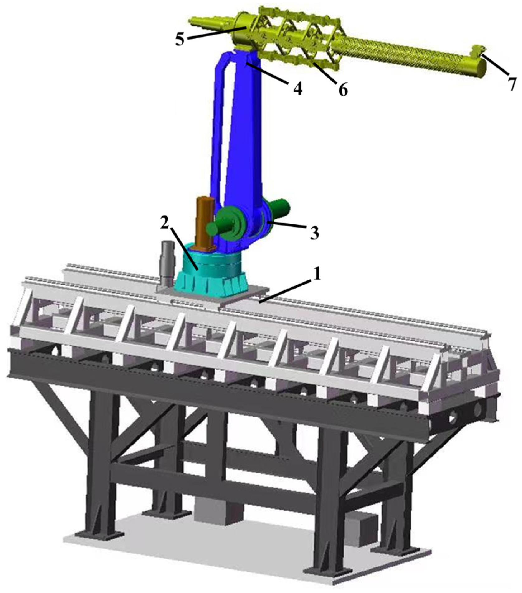
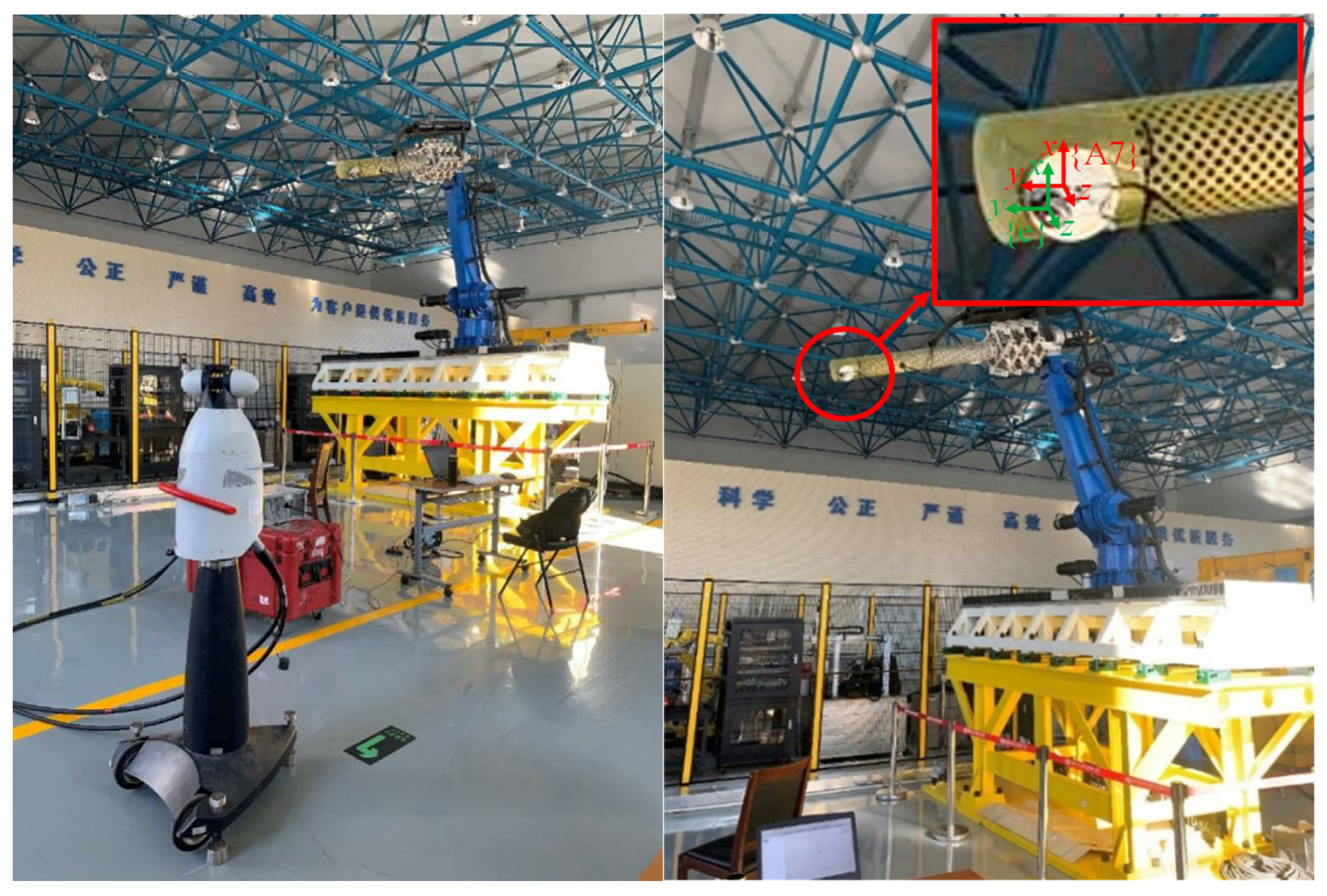
3.1. Introduction to Robot Configuration

The 3D model of the large-sized 7-DoF redundancy spray-painting robot is shown in Figure 1. The robot contains seven kinematic joints, including two motion joints and five rotation joints, and is a 7-DoF kinematic redundancy robot.

Figure 1. 3D model of the robot. For the convenience of description, the seven joints are numbered from 1 to 7, from the base to the terminal of the robot.

The base of the robot is connected to the pedestal through joint #1, which makes the robot capable of moving as a whole in the direction of the axis of the sprayed workpiece to realize the spraying of the whole surface of the sprayed workpiece. The base is connected to the waist through joint #2, which controls the robot’s swing in the lateral direction. The waist is connected to the main arm through joint #3, and the main arm is connected to the forearm through joint #4. Joints #3 and #4 are two rotation joints with their axes parallel and which control the angle of pitch of the main arm and forearm respectively. Joint #5 on the forearm controls the rotational movement of the forearm around its own axis. Joint #6 controls the telescopic movement of the forearm, which can increase its working space and flexibility without increasing the size of the robot. The spray gun is installed at the terminal of the forearm, and the direction of the spray gun is the same as the axis $x_7$, so joint #7 can control the angle between the pointing direction of the spray gun and the axis of the forearm. Joints #5 and #7 are two rotation joints with axes perpendicular to each other, which can ensure that the spray gun points in any direction in the space.

As can be observed from the 3D model of the robot shown in Figure 1, the drive motor of joint #4 utilizes a parallelogram four-rod mechanism on the main arm to transfer the motion to the forearm. By doing so, the motor on the forearm can be transferred to the head of the main arm, which can reduce the weight on the terminal as well as the inertia in the moving process, thus improving the flexibility and operational stability of the robot. The parallelogram four-rod mechanism is simplified in the subsequent section to reduce complexity. Since the driving connecting rod of the forearm near the head of the main arm and the forearm itself are opposite sides of the parallelogram, the motion of the two is similar. Therefore, in kinematic modeling, the four-rod mechanism can be ignored, and only the movement of the forearm relative to the main arm is considered.

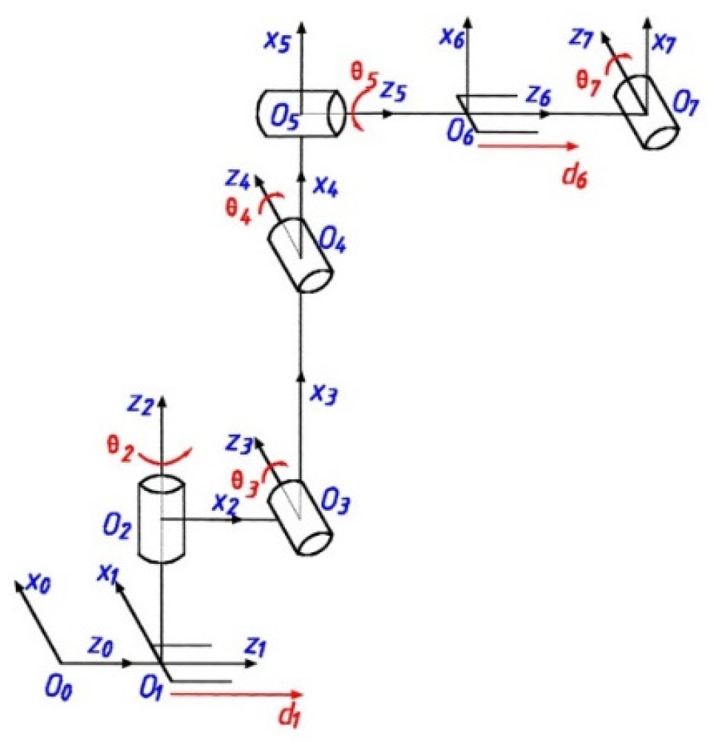
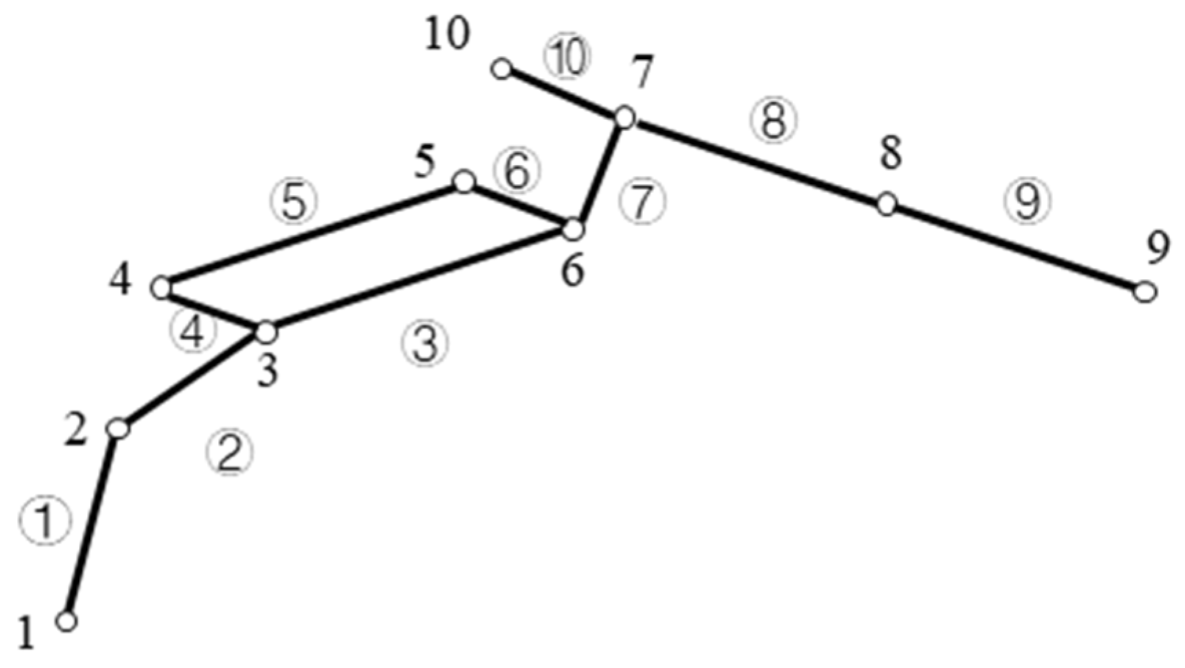
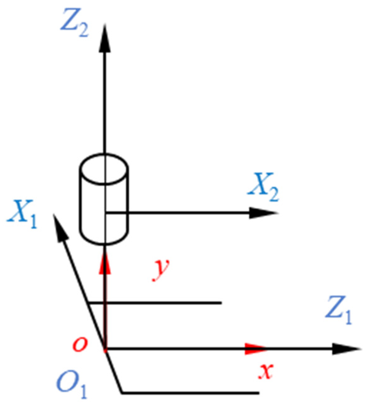
3.2. Forward Kinematic Modeling

The kinematic homogeneous transformation matrix of the robot is established using the D-H method, as shown in Figure 2.

Figure 2. Schematic of the robot mechanism.

According to the D-H method, the coordinate system of each rod is shown in Figure 2. Therefore, the relative position relationship between two adjacent rods can be described by four parameters: distance a_i−1 from axis Z_i−1 to axis Z_i along the direction of axis X_i−1, rotating angle α_i−1 from axis Z_i−1 to axis Z_i around axis X_i−1, distance d_i^* from axis X_i−1 to axis X_i along the direction of axis Z_i, and rotating angle θ_i from axis X_i−1 to axis X_i about axis Z_i. As a result, the homogeneous transformation matrix from the coordinate system O_i−1–X_i−1Y_i−1Z_i−1 to O_i−1–X_iY_iZ_i can be expressed as

$$\begin{array}{cc}\hfill {}^{i-1}{T}_i& =R_X({\alpha }_{i-1})D_X({\alpha }_{i-1})R_Z({\theta }_i)D_Z(d_i)\hfill \\ & =\left[\begin{array}{cccc}\cos {\theta }_i& -\sin {\theta }_i& 0& a_{i-1}\\ \sin {\theta }_i\cos {\alpha }_{i-1}& \cos {\theta }_i\cos {\alpha }_{i-1}& -\sin {\alpha }_{i-1}& -d_i\sin {\alpha }_{i-1}\\ \sin {\theta }_i\sin {\alpha }_{i-1}& \cos {\theta }_i\sin {\alpha }_{i-1}& \cos {\alpha }_{i-1}& d_i\cos {\alpha }_{i-1}\\ 0& 0& 0& 1\end{array}\right]\hfill \end{array}$$

(1)

$${}^0{T}_7{=}^0{T}_1{}^1{T}_2{}^2{T}_3{}^3{T}_4{}^4{T}_5{}^5{T}_6{}^6{T}_7=\left[\begin{array}{cccc}{n}_x& o_x& a_x& p_x\\ n_y& o_y& a_y& p_y\\ n_z& o_z& a_z& p_z\\ 0& 0& 0& 1\end{array}\right]$$

(2)

3.3. The MD-H Error Model

Since the third and fourth axes of the 7-DoF robot are parallel, the shortcomings of the D-H model shall be considered in error modeling. Therefore, the D-H model is improved by using 5-parameter MD-H modeling, which adds a rotation parameter β_i about the Y-axis to transform axis Z_i−1 to Z_i, thus avoiding the defects of the D-H model. The other parameter definitions of the improved model are the same as those of the D-H model. The joint deviation d_i^* is set to zero if the axes of two adjacent connecting rods are parallel. The rotation angle β_i is set to zero if the axes of two adjacent shores are not parallel. Then the MDH parameters of the robot are shown in Table 1. The coordinate transformation matrix of the improved model can be expressed as

$${}^{i-1}{T}_i=R_X({\alpha }_{i-1})D_X({\alpha }_{i-1})R_Z({\theta }_i)D_Z(d_i){\mathit{R}}_Y({\beta }_i)$$

(3)

Table 1. MD-H parameters of the robot.

Joint No.	${\mathit{a}}_{\mathit{i}-1}$/mm	${\mathit{\alpha }}_{\mathit{i}-1}$/°	${\mathit{d}}_{\mathit{i}}^{*}$/mm	${\mathit{\theta }}_{\mathit{i}}$/°	βi/°
#1	0	0	$d_1^{*}$	0	-
#2	0	−90	$d_2^{*}$	${\theta }_2$	-
#3	$a_2$	−90	0	${\theta }_3$	-
#4	$a_3$	0	0	${\theta }_4$	β4
#5	$a_4$	−90	0	${\theta }_5$	-
#6	0	0	$d_6^{*}$	0	-
#7	0	90	0	${\theta }_7$	-

4. Rigid-Flexible Coupling Error Model

4.1. Kinematic Error Model

Kinematic Error Model

By taking the differential of Equation (3), we can obtain

$${}^0{T}_7={\displaystyle \sum _{i=1}^7{}^0{T}_1{}^1{T}_2\cdots d^{i-1}{T}_i{\cdots }^6{T}_7}$$

(4)

Then, the total differential of Equation (4) can be calculated as

$$d^{i-1}{T}_i=\frac{{\partial }^{i-1}{T}_i}{\partial {\alpha }_{i-1}}\delta {\alpha }_{i-1}+\frac{{\partial }^{i-1}{T}_i}{\partial a_{i-1}}\delta a_{i-1}+\frac{{\partial }^{i-1}{T}_i}{\partial \theta }\delta \theta +\frac{{\partial }^{i-1}{T}_i}{\partial d}\delta d+\frac{{\partial }^{i-1}{T}_i}{\partial \beta }\delta \beta$$

(5)

To simplify Equation (5), dⁱ⁻¹T_i needs to be expressed as a function of ⁱ⁻¹T_i. Suppose that

$$\frac{{\partial }^{i-1}{T}_i}{\partial {\alpha }_{i-1}}{=}^{i-1}{T}_i{\mathit{D}}_{\alpha }; \frac{{\partial }^{i-1}{T}_i}{\partial a_{i-1}}{=}^{i-1}{T}_i{\mathit{D}}_a; \frac{{\partial }^{i-1}{T}_i}{\partial \theta }{=}^{i-1}{T}_i{\mathit{D}}_{\theta }; \frac{{\partial }^{i-1}{T}_i}{\partial d^{*}}{=}^{i-1}{T}_i{\mathit{D}}_{d^{*}};\frac{{\partial }^{i-1}{T}_i}{\partial \beta }{=}^{i-1}{T}_i{\mathit{D}}_{\beta }$$

(6)

where D_α, D_a, D_θ, D_d*, and D_β are coefficient matrices.

Combining Equations (5) and (6), we get

$$\begin{array}{ll}\hfill d^{i-1}{T}_i& {=}^{i-1}{T}_i{\mathit{D}}_{\alpha }\delta {\alpha }_{i-1}{+}^{i-1}{T}_i{\mathit{D}}_a\delta a_{i-1}{+}^{i-1}{T}_i{\mathit{D}}_{\theta }\delta {\theta }_i{+}^{i-1}{T}_i{\mathit{D}}_{d*}\delta d_i^{*}{+}^{i-1}{T}_i{\mathit{D}}_{\beta }\delta {\beta }_i\hfill \\ & {=}^{i-1}{T}_i\left({\mathit{D}}_{\alpha }\delta {\alpha }_{i-1}+{\mathit{D}}_a\delta a_{i-1}+{\mathit{D}}_{\theta }\delta {\theta }_i+{\mathit{D}}_{d*}\delta d_i+{\mathit{D}}_{\beta }\delta {\beta }_i\right)\hfill \end{array}$$

(7)

The differentiation by coordinates yields

$$d^{i-1}{T}_i{=}^{i-1}{T}_i{\mathit{\Delta }}_i$$

(8)

where Δ_i is the differential transformation matrix of the ith joint in the (i − 1)th joint coordinate system and can be expressed as

$${\mathit{\Delta }}_i=\left[\begin{array}{cccc}0& -\delta z_i& \delta y_i& \mathrm{d}{x}_i\\ \delta z_i& 0& -\delta x_i& \mathrm{d}{y}_i\\ -\delta y_i& \delta x_i& 0& \mathrm{d}{z}_i\\ 0& 0& 0& 0\end{array}\right]$$

(9)

where dx_i, dy_i, and dz_i correspond to differential translation, and δx_i, δy_i, and δz_i to differential rotation.

Combining Equations (7) and (8), we get

$${\mathit{D}}_i={\mathit{G}}_i{\mathit{E}}_i$$

(10)

where

$${\mathit{D}}_i=\left[\begin{array}{c}d{x}_i\\ d{y}_i\\ d{z}_i\\ \delta x_i\\ \delta y_i\\ \delta z_i\end{array}\right], {\mathit{G}}_i=\left[\begin{array}{cccc}-d_i^{*}s{\theta }_{i}c{\beta }_i& c{\theta }_{i}c{\beta }_i& 0& -s{\beta }_i\\ -d_i^{*}c{\theta }_i& -s{\theta }_i& 0& 0\\ -d_i^{*}s{\theta }_{i}s{\beta }_i& c{\theta }_{i}s{\beta }_i& 0& c{\beta }_i\\ c{\theta }_{i}c{\beta }_i& 0& -s{\beta }_i& 0\\ -s{\theta }_i& 0& 0& 0\\ c{\theta }_{i}s{\beta }_i& 0& c{\beta }_i& 0\end{array}\begin{array}{l}0\hfill \\ 0\hfill \\ 0\hfill \\ 0\hfill \\ 1\hfill \\ 0\hfill \end{array}\right], {\mathit{E}}_i=\left[\begin{array}{c}\delta {\alpha }_{i-1}\\ \delta a_{i-1}\\ \delta {\theta }_i\\ \begin{array}{l}\delta d_i\\ \delta {\beta }_i\end{array}\end{array}\right]$$

The terminal position error of the robot is the sum of the errors of different joints. Since the terminal position of the robot is measured in practical measurement, it is necessary to transform the errors of various joints into the robot terminal. Based on the principle of differential transformation of robots, the differential error transformation matrix from the ith joint coordinate system to the terminal coordinate system can be obtained as

$${}^i{\mathit{J}}_7=\left[\begin{array}{llllll}{n}_i^7{}_x\hfill & n_i^7{}_y\hfill & n_i^7{}_z\hfill & {(p_i^7\times n_i^7)}_x\hfill & {(p_i^7\times n_i^7)}_y\hfill & {(p_i^7\times n_i^7)}_z\hfill \\ o_i^7{}_x\hfill & o_i^7{}_y\hfill & o_i^7{}_z\hfill & {(p_i^7\times o_i^7)}_x\hfill & {(p_i^7\times o_i^7)}_y\hfill & {(p_i^7\times o_i^7)}_z\hfill \\ a_i^7{}_x\hfill & a_i^7{}_y\hfill & a_i^7{}_z\hfill & {(p_i^7\times a_i^7)}_x\hfill & {(p_i^7\times a_i^7)}_y\hfill & {(p_i^7\times a_i^7)}_z\hfill \\ 0\hfill & 0\hfill & 0\hfill & n_i^7{}_x\hfill & n_i^7{}_y\hfill & n_i^7{}_z\hfill \\ 0\hfill & 0\hfill & 0\hfill & o_i^7{}_x\hfill & o_i^7{}_y\hfill & o_i^7{}_z\hfill \\ 0\hfill & 0\hfill & 0\hfill & a_i^7{}_x\hfill & a_i^7{}_y\hfill & a_i^7{}_z\hfill \end{array}\right]$$

(11)

where n_i⁷, o_i⁷, a_i⁷, and p_i⁷ are the values of the transformation matrix from the ith joint coordinate system to the terminal coordinate system. Then, we can obtain the terminal errors induced by joint i as

$${\mathit{e}}_i^7={}^i{\mathit{J}}_7{\mathit{G}}_i{\mathit{E}}_i$$

(12)

The total terminal error induced by all joints can be obtained by

$$\mathit{e}={\displaystyle \sum _{i=0}^7{}^i{\mathit{J}}_7{\mathit{G}}_i{\mathit{E}}_i}=\mathit{J}d\mathit{r}$$

(13)

where dr denotes the total error obtained by summing the errors of the D-H parameters.

4.2. Analysis of Redundancy Kinematic Error of Robots

According to the correlation between the column vectors of the Jacobian matrix, errors can be divided into: independent, correlated, and nonfunctional errors. Independent error refers to an error that can be identified directly, reflected in the fact that the corresponding column of the error is not linearly correlated with other columns of the Jacobian matrix. The correlated error implies that the corresponding error column is linearly correlated with other columns of the Jacobian matrix. Given the interaction of each other during the identification process, only one of them is retained. The nonfunctional error refers to an error that does not affect the terminal error, and since this parameter cannot be identified, it needs to be eliminated.

The transformation matrix from any joint i coordinate system to the base coordinate system of the robot can be expressed as

$${}_i{}^0\mathit{T}=\left[\begin{array}{llll}{\mathit{n}}_i\hfill & {\mathit{o}}_i\hfill & {\mathit{a}}_i\hfill & {\mathit{p}}_i\hfill \\ 0\hfill & 0\hfill & 0\hfill & 1\hfill \end{array}\right]$$

(14)

The transformation matrix from the previous joint coordinate system i−1 to the base coordinate system of the robot is

$${}_{i-1}{}^0\mathit{T}=\left[\begin{array}{llll}{\mathit{n}}_{i-1}\hfill & {\mathit{o}}_{i-1}\hfill & {\mathit{a}}_{i-1}\hfill & {\mathit{p}}_{i-1}\hfill \\ 0\hfill & 0\hfill & 0\hfill & 1\hfill \end{array}\right]$$

(15)

The relationship between the two coordinate systems can be expressed as

$${}_i{}^0\mathit{T}={}_{i-1}{}^0\mathit{T}\left[\begin{array}{cccc}\cos {\theta }_i& -\sin {\theta }_i& 0& a_{i-1}\\ \sin {\theta }_i\cos {\alpha }_{i-1}& \cos {\theta }_i\cos {\alpha }_{i-1}& -\sin {\alpha }_{i-1}& -d_i\sin {\alpha }_{i-1}\\ \sin {\theta }_i\sin {\alpha }_{i-1}& \cos {\theta }_i\sin {\alpha }_{i-1}& \cos {\alpha }_{i-1}& d_i\cos {\alpha }_{i-1}\\ 0& 0& 0& 1\end{array}\right]$$

(16)

Thus, the column vectors in the transformation matrix can be written as

$$\begin{array}{l}{\mathit{n}}_i=c{\theta }_i\cdot {\mathit{n}}_{i-1}+s{\theta }_{i}c{\alpha }_{i-1}\cdot {\mathit{o}}_{i-1}+s{\theta }_{i}s{\alpha }_{i-1}\cdot {\mathit{a}}_{i-1}\\ {\mathit{o}}_i=-s{\theta }_i\cdot {\mathit{n}}_{i-1}+c{\theta }_{i}c{\alpha }_{i-1}\cdot {\mathit{o}}_{i-1}+c{\theta }_{i}s{\alpha }_{i-1}\cdot {\mathit{a}}_{i-1}\\ {\mathit{a}}_i=-s{\alpha }_{i-1}\cdot {\mathit{o}}_{i-1}+c{\alpha }_{i-1}\cdot {\mathit{a}}_{i-1}\\ {\mathit{p}}_i=a_{i-1}\cdot {\mathit{n}}_{i-1}-d_{i}s{\alpha }_{i-1}\cdot {\mathit{o}}_{i-1}+d_{i}c{\alpha }_{i-1}\cdot {\mathit{a}}_{i-1}+{\mathit{p}}_{i-1}\end{array}$$

(17)

The Jacobian matrix J is obtained by taking the total differential of all the kinematic parameters, and J_ai−1, J_αi−1, J_di, J_θ1, and J_βi indicate the five columns of the Jacobian matrix corresponding to the five D-H parameters, respectively. Then, the Jacobian matrix J can be expressed as

$$\mathit{J}=\left[\begin{array}{lllll}{\mathit{J}}_{ai-1}\hfill & {\mathit{J}}_{\alpha i-1}\hfill & {\mathit{J}}_{di}\hfill & {\mathit{J}}_{\theta i}\hfill & {\mathit{J}}_{\beta i}\hfill \end{array}\right]$$

(18)

According to the differential kinematics of robots, the column vectors of the Jacobian matrix at any joint can be expressed as the cross-product of vectors.

$${\mathit{J}}_{ai-1}=\left[\begin{array}{c}{\mathit{n}}_{i-1}\\ 0\end{array}\right],{\mathit{J}}_{\alpha i-1}=\left[\begin{array}{c}{\mathit{n}}_{i-1}\times {}^{i-1}p_n^0\\ {\mathit{n}}_{i-1}\end{array}\right],{\mathit{J}}_{di}=\left[\begin{array}{c}{\mathit{a}}_i\\ 0\end{array}\right],{\mathit{J}}_{\theta i}=\left[\begin{array}{c}{\mathit{a}}_i\times {}^{i}p_n^0\\ {\mathit{a}}_i\end{array}\right],{\mathit{J}}_{\beta i}=\left[\begin{array}{c}{\mathit{o}}_i\times {}^{i}p_n^0\\ {\mathit{o}}_i\end{array}\right]$$

(19)

By combining these equations, we get

$$\begin{array}{l}{\mathit{J}}_{ai}=c{\theta }_i\cdot {\mathit{J}}_{ai-1}+s{\theta }_{i}c{\alpha }_{i-1}\left[\begin{array}{c}{\mathit{o}}_{i-1}\\ {\mathit{0}}_{1\times 3}\end{array}\right]+s{\theta }_{i}s{\alpha }_{i-1}{\mathit{J}}_{di-1};\\ {\mathit{J}}_{di}=c{\alpha }_{i-1}{\mathit{J}}_{di-1}-s{\alpha }_{i-1}\left[\begin{array}{c}{\mathit{o}}_{i-1}\\ {\mathit{0}}_{1\times 3}\end{array}\right];\\ {\mathit{J}}_{\alpha i}=-d_{i}s{\theta }_i{\mathit{J}}_{ai-1}+(a_{i-1}c{\alpha }_{i-1}s{\theta }_i+d_{i}s{\alpha }_{i-1}c{\theta }_i){\mathit{J}}_{di-1}+c{\theta }_i{\mathit{J}}_{\alpha i-1}+s{\theta }_{i}c{\alpha }_{i-1}{\mathit{J}}_{\beta i-1}+\\ s{\theta }_{i}s{\alpha }_{i-1}{\mathit{J}}_{\theta i-1}+(-a_{i-1}s{\theta }_{i}s{\alpha }_{i-1}+d_{i}c{\theta }_{i}c{\alpha }_{i-1})\left[\begin{array}{c}{\mathit{o}}_{i-1}\\ {\mathit{0}}_{1\times 3}\end{array}\right];\\ {\mathit{J}}_{\theta i}=-a_{i-1}c{\alpha }_{i-1}\left[\begin{array}{c}{\mathit{o}}_{i-1}\\ {\mathit{0}}_{1\times 3}\end{array}\right]-a_{i-1}s{\alpha }_{i-1}{\mathit{J}}_{ai-1}-s{\alpha }_{i-1}{\mathit{J}}_{\beta i-1}+c{\alpha }_{i-1}{\mathit{J}}_{\theta i-1};\\ {\mathit{J}}_{\beta i}=-d_{i}c{\theta }_i{\mathit{J}}_{ai-1}+(-a_{i-1}s{\alpha }_{i-1}c{\theta }_i-d_{i}c{\alpha }_{i-1}s{\theta }_i)\left[\begin{array}{c}{\mathit{o}}_{i-1}\\ {\mathit{0}}_{1\times 3}\end{array}\right]-s{\theta }_i{\mathit{J}}_{\alpha i-1}+c{\theta }_{i}c{\alpha }_{i-1}{\mathit{J}}_{\beta i-1}+\\ s{\alpha }_{i-1}c{\theta }_i{\mathit{J}}_{\theta i-1}+(-d_{i}s{\theta }_{i}s{\alpha }_{i-1}+a_{i-1}c{\theta }_{i}c{\alpha }_{i-1}){\mathit{J}}_{di-1};\end{array}$$

(20)

Substituting the theoretical values of the kinematic parameters into the above equations, the following conditions can be derived:

• If α_i−1 ≠ 0, a redundancy error is present;
• If α_i−1 = 0 and a_i−1 ≠ 0, δd_i−1^* and δd_i^* are mutually redundant, and either shall be eliminated, and δβ_i shall be introduced for identification.
• If α_i−1 = 0 and a_i−1 = 0, δd_i−1^* and δd_i^* are mutually redundant, and δθ_i−1 and δθ_i are mutually redundant, and some parameters shall be eliminated.
• If θ_i = 0 and d_i^* ≠ 0, δa_i−1 and δa_i are mutually redundant, and some parameters shall be eliminated.
• If θ_i = 0 and d_i^* = 0, δα_i−1 and δα_i are mutually redundant and δa_i−1 and δa_i are mutually redundant, and some parameters shall be eliminated.
• After eliminating redundant parameters, the D-H parameter error still contains 24 errors.

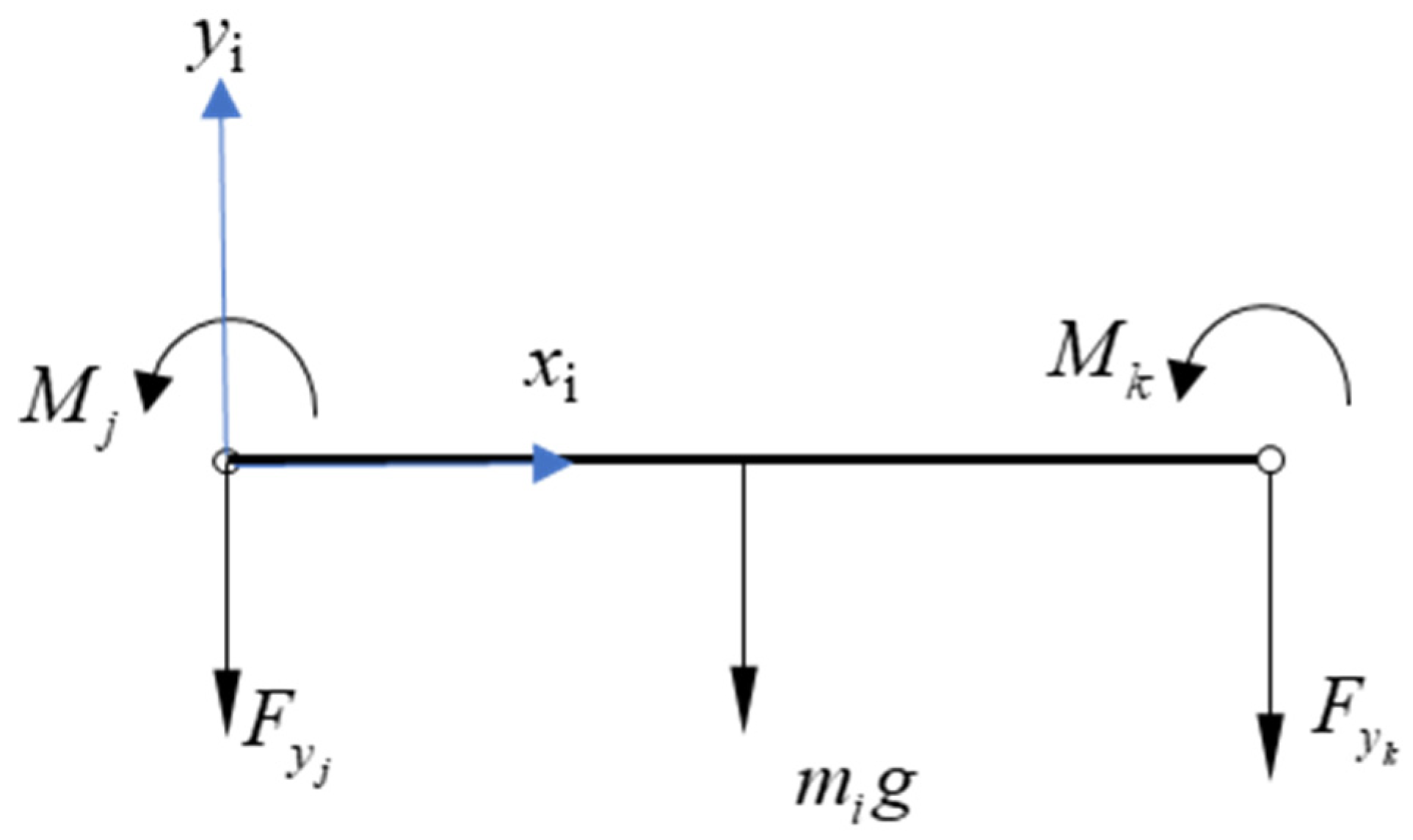
5. Static Stiffness Error Model

5.1. Static Stiffness Model

The overall structure of the robotic arm is simplified to a structure with ten nodes and ten beam units, as shown in Figure 3.

Figure 3. Structure of the robotic arm. 1–9 indicates the node numbers and ①–⑨ the numbering of the beam units.

The part between joints #1 and #2 is considered the first beam unit, Unit 1; the part between joints #2 and # 3 is regarded as the second beam unit (Unit 2). The main arm between joints #3 and #4 is the third unit (Unit 3). The connecting rod between joint #3 and the forearm is the fourth unit (Unit 4). The forearm is regarded as the fifth unit (Unit 5). Unit 8 is the telescopic sleeve of the original robotic arm and the hinge mechanism; the connecting rod between joint #7 and the hinge is considered the tenth unit (Unit 10). Unit 7 is perpendicular to both Units 8 and 6, respectively. Units 3, 4, 5, and 6 form a parallelogram mechanism. The mass of Unit i is assumed to be m_i (unit: kg), the length is considered to be l_i (unit: m), and, in particular, the length of Unit 9 l₉ = l_o + d₆^* (l_o is the length of the hinge when d₆^* = 0 holds in the D-H coordinate system).

As shown in Figure 4, the finite element global coordinate system is defined as follows: the origin of the finite element global coordinate system o–XY coincides with the origin O₁ of O₁–X₁Y₁Z₁ in the robotic arm D-H coordinate system, the x-direction always coincides with the X₂-direction of O₁–X₂Y₂Z₂ in the robotic arm coordinate system. The y-direction is opposite to the gravity direction.

Figure 4. Finite element global coordinate system of the robotic arm.

The local coordinate systems are established based on the following principles. Since each unit contains nodes j and k (both satisfying i < j), node j is set as the origin of the local coordinate system, and the direction from node j to node k is set as the positive direction of the x-axis of the local coordinate system of this unit, and the axis obtained by rotating the x-axis π/2 counterclockwise is set as the y-axis.

Since only the robotic arm’s deformation under gravity is considered, the theory of small deformation assumption is used here. The uniform load can be converted into the load on the node by the equivalence principle. For Unit i, when the x-direction of the local coordinate system of the unit is the same as the horizontal direction, the equivalent load on the node is as follows (the nodal force is positive in tension, and the bending moment is positive if it is counterclockwise):

Herein, F_yj = F_yk = 1/2 m_ig (the concentrated load is positive, which means that the direction is the same as that shown in Figure 5, and the same for the following bending moment), M_j = –1/12 m_igl_i, and M_k = 1/12 m_igl_i.

Figure 5. Equivalent diagram of uniform load.

Based on the established global coordinate system and the local coordinate systems of different units, we assume the angle between the local coordinate system of each unit and the finite element global coordinate system as

$${\beta }^{*}={[\begin{array}{cccc}{\beta }_1^{*}& {\beta }_2^{*}& \cdots & {\beta }_{10}^{*}\end{array}]}^T$$

(21)

where β_i^* is the angle between the local coordinate system x_iy_i of Unit i and the finite element global coordinate system o–XY and is positive if the finite element global coordinate system rotates toward the local coordinate system counterclockwise. In vector β^*, β₁^* = π/2, and β₂^* is a non-zero fixed value, which can be obtained by measuring the geometric relationship of the robotic arm structure. Besides, some elements of the vector β^* can be described by the variables of the robotic arm in the D-H coordinate system, and some elements of the vector can be expressed as

$$\{\begin{array}{l}{\beta }_3^{*}={\theta }_3\hfill \\ {\beta }_7^{*}={\theta }_3+{\theta }_4\hfill \\ {\beta }_8^{*}={\beta }_9^{*}={\beta }_{10}^{*}={\theta }_3+{\theta }_4-\pi /2\hfill \end{array}$$

(22)

Based on the geometric relationship of each unit in Figure 3, we get

$$\{\begin{array}{l}{\beta }_4^{*}={\theta }_3+{\theta }_4+\pi /2\hfill \\ {\beta }_5^{*}={\theta }_3\hfill \\ {\beta }_6^{*}={\theta }_3+{\theta }_4-\pi /2\hfill \end{array}$$

(23)

Assuming that the stiffness matrix of Unit i in its respective local coordinate system is K_i, then the stiffness matrix of this unit in the finite element global coordinate system is

$${\overline{K}}_i=T_i{}^T{K}_i{T}_i$$

(24)

where matrix T_i is

$$T_i=\left[\begin{array}{cccccc}\cos {\beta }_i^{*}& -\sin {\beta }_i^{*}& 0& 0& 0& 0\\ \sin {\beta }_i^{*}& \cos {\beta }_i^{*}& 0& 0& 0& 0\\ 0& 0& 1& 0& 0& 0\\ 0& 0& 0& \cos {\beta }_i^{*}& -\sin {\beta }_i^{*}& 0\\ 0& 0& 0& \sin {\beta }_i^{*}& \cos {\beta }_i^{*}& 0\\ 0& 0& 0& 0& 0& 1\end{array}\right]$$

(25)

Since the stiffness of Unit 9 changes with the stretching and rotation (i.e., parameters θ₅ and d₆^*) of the hinge, the stiffness matrix of Unit 9 can be expressed θ₅ about and d₆^* as

$$K_9=\left[\begin{array}{ccc}{f}_{11}(d_6)g_{11}({\theta }_5)& f_{12}(d_6)g_{12}({\theta }_5)& f_{13}(d_6)g_{13}({\theta }_5)\\ f_{21}(d_6)g_{21}({\theta }_5)& f_{22}(d_6)g_{22}({\theta }_5)& f_{23}(d_6)g_{23}({\theta }_5)\\ f_{31}(d_6)g_{31}({\theta }_5)& f_{32}(d_6)g_{11}({\theta }_5)& f_{33}(d_6)g_{33}({\theta }_5)\end{array}\right]$$

(26)

Herein, the coefficients can be fitted using the stiffness matrix data of Unit 9 extracted in the MySQL Workbench tool. It is assumed that the displacement and load on the ith node under the finite element global coordinate system are as follows:

$$q_i=\left[\begin{array}{ccc}{u}_i& v_i& {\phi }_i\end{array}\right]$$

(27)

$$F_i=\left[\begin{array}{ccc}{F}_{xi}& F_{yi}& M_i\end{array}\right]$$

(28)

In Equation (27), the unit of u_i and v_i is m, and the unit of φ_i is rad. Then, the displacement of the whole structure and the load on it under the finite element global coordinate system can be expressed as

$$q={[\begin{array}{cccc}{q}_1& q_2& \cdots & q_{10}\end{array}]}^T$$

(29)

$$F={[\begin{array}{cccc}{F}_1& F_2& \cdots & F_{10}\end{array}]}^T$$

(30)

Assuming that the overall stiffness matrix is $\widehat{K}$, then

$$\widehat{K}q=F$$

(31)

Since only the impact of gravity on each unit is considered, the load on each beam is uniform. Additionally, the y-direction of the finite element global coordinate system is the same as the direction of gravity. Therefore, analyzing the nodes under the finite element global coordinate system is more straightforward. Since there is no load in the x-direction of the system under the global coordinate system, the force in the x-direction of each node under the global coordinate system must be zero, i.e.,

$$F_{xi}=0$$

(32)

For all nodes except Node 1, the gravity equivalent load on each node is the overall load on the node under the finite element global coordinate system. As seen from the load-equivalent diagram shown in Figure 6, the overall load of all nodes except Node 1 is

$$\begin{gathered} F_i=\left[\begin{array}{ccc}0& -\frac{1}{2}(m_{i-1}+m_i)g& \frac{1}{12}g(m_{i-1}{l}_{i-1}\cos {\beta }_{i-1}-m_i{l}_i\cos {\beta }_i)\end{array}\right] i = 2, 4, 5, 7, 8, 9 \\ {F}_i=\left[\begin{array}{ccc}0& -\frac{1}{2}(m_{i-1}+m_i+m_{i+1})g& \frac{1}{12}g(m_{i-i}{l}_{i-1}\cos {\beta }_{i-1}-m_i{l}_i\cos {\beta }_i-m_{i+1}{l}_{i+1}\cos {\beta }_{i+1})\end{array}\right] i = 3, 6 \\ {F}_{10}=\left[\begin{array}{ccc}0& -\frac{1}{2}{m}_{10}g& \frac{1}{12}{m}_{10}g{l}_{10}\cos {\beta }_{10}\end{array}\right] \end{gathered}$$

(33)

Figure 6. Flowchart of error compensation of 7-DoF spray-painting robots.

Since Node 1 has fixed support, the impact of F₁ on terminal deflection can be ignored. The displacement and angle of rotation of each node can be obtained by eliminating the corresponding rows and columns of $\widehat{\mathit{K}}\mathit{q}=\mathit{F}$using boundary conditions.

Since each node corresponds to a joint of the robotic arm, and the joint is the origin of each coordinate in the D-H coordinate system. Therefore, under the influence of gravity, the origin of the D-H coordinate system of the joint where Node j is located is translated along the translation vector λ_i = [u_i v_i 0] under the finite element global coordinate system and rotated along the direction vector p in the z-direction of the finite element global coordinate system with the angle of rotation φ_i.

It is assumed that the element’s coordinate system of the robotic arm, without taking the effect of gravity into account, is O_jX_jY_jZ_j and the terminal’s element coordinate system with the impact of gravity considered is O_j^ʹX_j^ʹY_j^ʹZ_j^ʹ. Here, the homogeneous transformation matrix from the coordinate system O₇X₇Y₇Z₇ to the coordinate system O₇^ʹX₇^ʹY₇^ʹZ₇^ʹ is defined as ⁷T_7’.

Given that Node 9 is the origin O₇ of the coordinate system O₇X₇Y₇Z₇, the translation vector of the coordinate system O₇X₇Y₇Z₇ under the finite element global coordinate system is

$${\lambda }_9=\left[\begin{array}{ccc}{u}_9& v_9& 0\end{array}\right]$$

(34)

Likewise, λ₉ is expressed as ⁷λ₉ under the coordinate system O₇X₇Y₇Z₇.

$${}^7\lambda _9={({}^{2}R_3{}^{3}R_4{}^{4}R_5{}^{5}R_6{}^{6}R_7)}^T{}^{2}R\lambda _9$$

(35)

Then, we can obtain the homogeneous transformation matrix ⁷T_7ʹ from the coordinate system O₇X₇Y₇Z₇ to the coordinate system O₇^ʹX₇^ʹY₇^ʹZ₇^ʹ as

$${}^7\mathit{T}_{7\prime }=\left[\begin{array}{cc}{}^7\mathit{R}_{7\prime }& {}^7\mathsf{\lambda }_9\\ O_{1\times 3}& 1\end{array}\right]$$

(36)

where O_1×3 is a 0 matrix with one row and three columns. For the end displacement p₇ = [σ_x7 σ_y7 σ_z7], parameter ^7ʹR₇ is derived as follows:

$${}^7{R}_{7^{\prime }}=\left[\begin{array}{ccc}{\sigma }_{x_7}{\sigma }_{x_7}(1-c{\phi }_9)+c{\phi }_9& {\sigma }_{x_7}{\sigma }_{y_7}(1-c{\phi }_9)+{\sigma }_{z_7}s{\phi }_9& {\sigma }_{x_7}{\sigma }_{z_7}(1-c{\phi }_9)-{\sigma }_{y_7}s{\phi }_9\\ {\sigma }_{x_7}{\sigma }_{z_7}(1-c{\phi }_9)-{\sigma }_{z_7}s{\phi }_9& {\sigma }_{y_7}{\sigma }_{x_7}(1-c{\phi }_9)+c{\phi }_9& {\sigma }_{y_7}{\sigma }_{z_7}(1-c{\phi }_9)+{\sigma }_{x_7}s{\phi }_9\\ {\sigma }_{x_7}{\sigma }_{z_7}(1-c{\phi }_9)+{\sigma }_{z_7}s{\phi }_9& {\sigma }_{y_7}{\sigma }_{z_7}(1-c{\phi }_9)-{\sigma }_{x_7}s{\phi }_9& {\sigma }_{z_7}{\sigma }_{z_7}(1-c{\phi }_9)+c{\phi }_9\end{array}\right]$$

(37)

where cφ₉ = cos(φ₉) and sφ₉ = sin(φ₉).

5.2. Rigid-Flexible Coupling Kinematic Error Model

In the rigid-flexible coupling kinematic error model, only the influence of the joint’s driving direction error on the gravity model is retained, and the effect of other geometric errors on gravitational deformation is neglected. When gravitational deformation is not considered, the Jacobian matrix can be written as $\mathit{e}={\displaystyle \sum _{i=0}^7}{}^i\mathit{J}_7{\mathit{G}}_i{\mathit{E}}_i=\mathit{J}d\mathit{r}$, where e is the error transformed into the seventh coordinate system. However, when gravitational deformation exists, since gravitational deformation is a small quantity of first order, and the deviation caused by the mechanism geometric error is also a small quantity of first order, the variation of gravitational deformation caused by the geometric error is a high-order error and thus can be ignored. Therefore, the gravitational deformation of nominal parameters and the parameters compensated in the driving direction are used for calculation in this study.

When the gravity model is considered, the joint coordinate system needs to be transformed using the homogeneous transformation matrix ⁱ⁻¹T_iʹ of gravitational deformation of nominal parameters and the parameters compensated in the driving direction. The errors of the terminal coordinate system can be obtained.

Assuming that

$${}^7{T}_{7^{\prime }}=\left[\begin{array}{cccc}{n}_x{}^{’}& o_x{}^{’}& a_x{}^{’}& p_x{}^{’}\\ n_y{}^{’}& o_y{}^{’}& a_y{}^{’}& p_y{}^{’}\\ n_z{}^{’}& o_z{}^{’}& a_z{}^{’}& p_z{}^{’}\\ 0& 0& 0& 1\end{array}\right]$$

(38)

then,

$${\mathit{J}}^{’}=\left[\begin{array}{llllll}{n}_x{}^{’}\hfill & n_y{}^{’}\hfill & n_z{}^{’}\hfill & {(p^{’}\times n^{’})}_x\hfill & {(p^{’}\times n^{’})}_y\hfill & {(p^{’}\times n^{’})}_z\hfill \\ o_x{}^{’}\hfill & o_y{}^{’}\hfill & o_z{}^{’}\hfill & {(p^{’}\times o^{’})}_x\hfill & {(p^{’}\times o^{’})}_y\hfill & {(p^{’}\times o^{’})}_z\hfill \\ a_x{}^{’}\hfill & a_y{}^{’}\hfill & a_z{}^{’}\hfill & {(p^{’}\times a^{’})}_x\hfill & {(p^{’}\times a^{’})}_y\hfill & {(p^{’}\times a^{’})}_z\hfill \\ 0\hfill & 0\hfill & 0\hfill & n_x{}^{’}\hfill & n_y{}^{’}\hfill & n_z{}^{’}\hfill \\ 0\hfill & 0\hfill & 0\hfill & o_x{}^{’}\hfill & o_y{}^{’}\hfill & o_z{}^{’}\hfill \\ 0\hfill & 0\hfill & 0\hfill & a_x{}^{’}\hfill & a_y{}^{’}\hfill & a_z{}^{’}\hfill \end{array}\right]$$

(39)

The error vector described in the terminal coordinate system with gravitational deformation taken into consideration is:

$$\mathit{e}\prime ={\mathit{J}}^{\prime }\mathit{e}={\displaystyle \sum _{i=0}^7}{\mathit{J}}^{\prime }{}^i\mathit{J}_7{\mathit{G}}_i{\mathit{E}}_i={\mathit{J}}^{*}(d\mathit{r})$$

(40)

where J^* is the Jacobian matrix of error with gravitational deformation taken into consideration. After the measured terminal error is estimated, one can determine the geometric error from J^*, which, in turn, is calculated via the regularized least squares method [29,30].

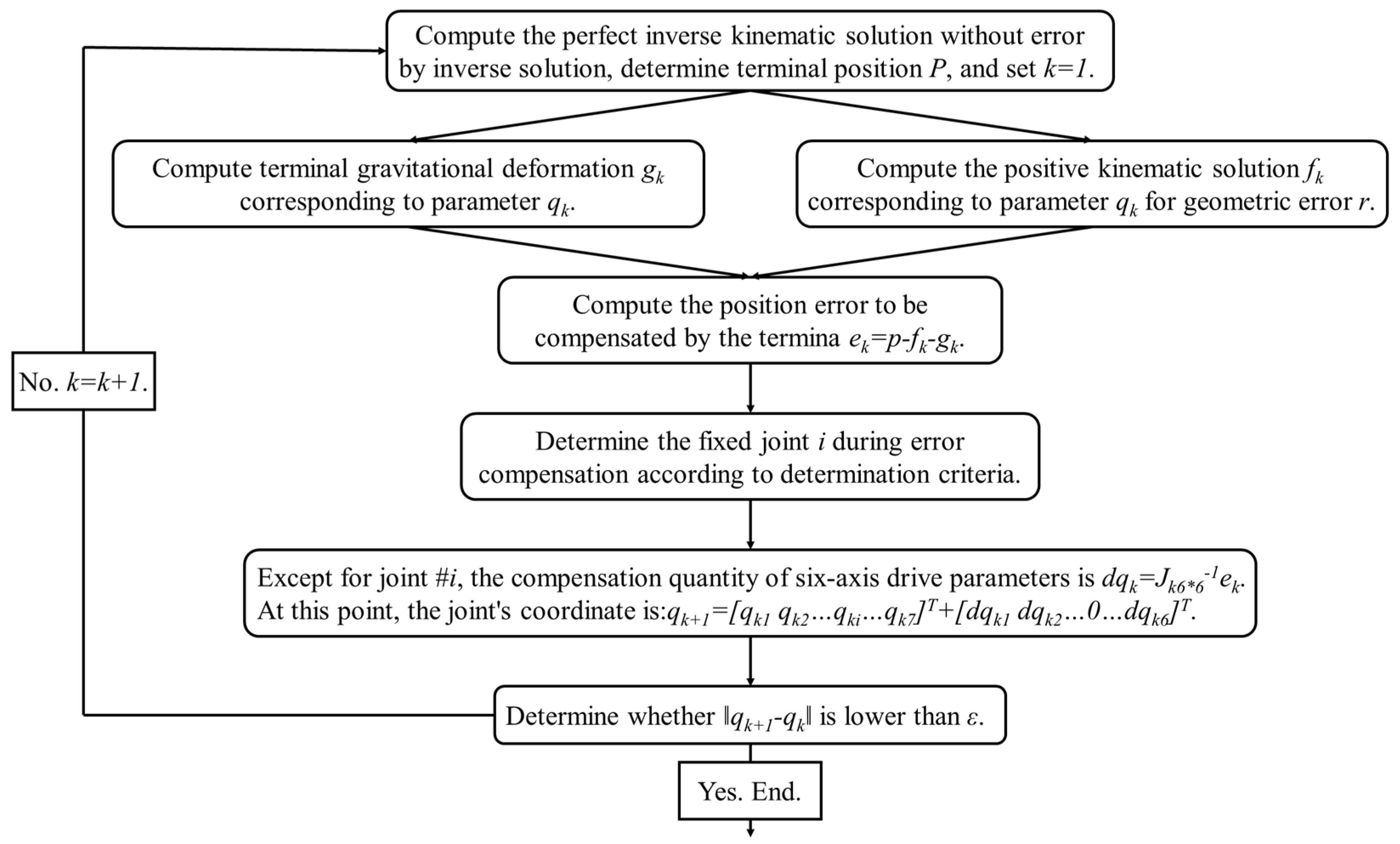
6. Error Compensation Strategy for 7-DoF Hybrid Spray-Painting Robots

After kinematic calibration, an error compensation strategy was proposed for the 7-DoF spray-painting robot. The proposed approach solves the inverse motion with errors based on the optimized inverse motion solution. Therefore, the inverse motion with errors also should be optimized in the same direction as the inverse kinematic solution.

Since the inverse motion with errors could not be solved directly using the analytical formula, the inverse kinematic solution with errors was obtained via the Jacobian matrix iteration method. Since the robot contained seven joints and redundant joints resulted in no inverse of the 6 × 7 Jacobian matrix, only six joints were needed to compensate for the identified errors in calibration. Properly selecting the fixed joint is the key to the iteration process.

In solving the inverse kinematics without errors, Wang et al. [45] used inertia volatility as an optimization index, which was found instrumental in solving the inverse kinematics with errors. For kinematic optimization, determination criteria were set, the inertia load sensitivity of the joint corresponding to the unit end error was defined to represent the change of inertia load when the single joint motion compensates for the unit error of the end, and it was taken as the determination index, providing the basis for solving the inverse kinematic solution with errors. The iteration process was as follows.

Herein, the initial value of the Jacobi iteration is the optimized inverse kinematic solution. For a given terminal position p and a given geometric error r, the joint drive variable q = [q₁ q₂ q₃ q₄ q₅ q₆ q₇]^T can be computed using the numerical method.

When solving the inertial load sensitivity of the joint corresponding to the unit error, the inertial load sensitivity should be solved first. In solving the inertial load sensitivity, to consider the overall effect of a joint on the inertial load, the average inertial load over the entire working space of the remaining joints needs to be computed when each joint of the mechanism takes different values. In this study, given the coordinate of a joint, the inertial loads of the remaining six joints were obtained, integrated about their coordinates, and divided by the length of the integration interval of the remaining six joints to get the average inertia matrix in the entire working space. The inertia matrix was only related to the robot’s posture but not to the translational motion of the base, so only Joints #2, #3, #4, #5, and #7 had to be calculated. With joint #6 taken as an example, the variation of the inertia load on joint #6 in extension was as follows:

$$\overline{M}(d_6^{*})=\frac{{\displaystyle {\int }_{{\theta }_{7l}}^{{\theta }_{7u}}{\displaystyle {\int }_{{\theta }_{5l}}^{{\theta }_{5u}}{\displaystyle {\int }_{{\theta }_{4l}}^{{\theta }_{4u}}{\displaystyle {\int }_{{\theta }_{3l}}^{{\theta }_{3u}}{\displaystyle {\int }_{{\theta }_{2l}}^{{\theta }_{2u}}{M}_m(q)d{\theta }_{2}d{\theta }_{3}d{\theta }_{4}d{\theta }_{5}d{\theta }_7}}}}}}{{\displaystyle {\int }_{{\theta }_{2l}}^{{\theta }_{2u}}d{\theta }_2\cdot {\displaystyle {\int }_{{\theta }_{3l}}^{{\theta }_{3u}}d{\theta }_3\cdot }{\displaystyle {\int }_{{\theta }_{4l}}^{{\theta }_{4u}}d{\theta }_4\cdot }{\displaystyle {\int }_{{\theta }_{5l}}^{{\theta }_{5u}}d{\theta }_5\cdot }{\displaystyle {\int }_{{\theta }_{7l}}^{{\theta }_{7u}}d{\theta }_7}}}$$

(41)

where M_m(q) is the inertia matrix of the current joint coordinates, θ_u is the upper joint boundary, and θ_l is the lower joint boundary. The conformation shows that joints #3, #4, and #6 are more influential than the others, mainly comparing these three joints. The impact of the inertial load on joints #3, #4, and #6 is shown in Figure 7, where the slope is the inertia sensitivity.

Figure 7. Inertial load effect of kinematics of joint 3—(a), joint 4—(b), joint 6—(c).

Secondly, to compare the single joint motion under the unit end error and define the joint sensitivity index. Since this index is affected by the pose of the end, its solution is complicated. In order to simplify the calculation, the joint zero sensitivity index is defined as (with joint #6 taken as an example):

$$\mathrm{S}(d_6)=\frac{{\displaystyle {\int }_{{\theta }_{7l}}^{{\theta }_{7u}}{\displaystyle {\int }_{{\theta }_{5l}}^{{\theta }_{5u}}{\displaystyle {\int }_{{\theta }_{4l}}^{{\theta }_{4u}}{\displaystyle {\int }_{{\theta }_{3l}}^{{\theta }_{3u}}{\displaystyle {\int }_{{\theta }_{2l}}^{{\theta }_{2u}}{\left|\right|\mathrm{J}}_6(q)\left|\right|d{\theta }_{2}d{\theta }_{3}d{\theta }_{4}d{\theta }_{5}d{\theta }_7}}}}}}{{\displaystyle {\int }_{{\theta }_{2l}}^{{\theta }_{2u}}d{\theta }_2\cdot {\displaystyle {\int }_{{\theta }_{3l}}^{{\theta }_{3u}}d{\theta }_3\cdot }{\displaystyle {\int }_{{\theta }_{4l}}^{{\theta }_{4u}}d{\theta }_4\cdot }{\displaystyle {\int }_{{\theta }_{5l}}^{{\theta }_{5u}}d{\theta }_5\cdot }{\displaystyle {\int }_{{\theta }_{7l}}^{{\theta }_{7u}}d{\theta }_7}}}$$

(42)

where J₆(q) denotes the column corresponding to d6 in the driving Jacobi matrix, Then, the inertia load sensitivity of the joint corresponding to the unit end error can be expressed as:

$$M_{d_6^{*}}^{*}=\frac{d\overline{M}(d_6^{*})}{d{d}_6^{*}\cdot S(d_6^{*})}$$

(43)

The inertia sensitivity of joint 6 is relatively high (the slope is relatively high), as shown in Figure 7. The calculated ratio of joint sensitivity of joint 3, 4 and 6 is 2.369:1.647:1. Joint 6 has the minimum joint sensitivity and the maximum inertia sensitivity, so the unit end error of joint 6 corresponds to the maximum inertia load sensitivity of the joint. In this case, according to the optimization direction of inverse motion, Joint #6 was taken as a fixed joint. Then, the coordinates of the seven joints were obtained, and commands were directly entered into the robot for compensation.

7. Experimental Methods and Data Analysis

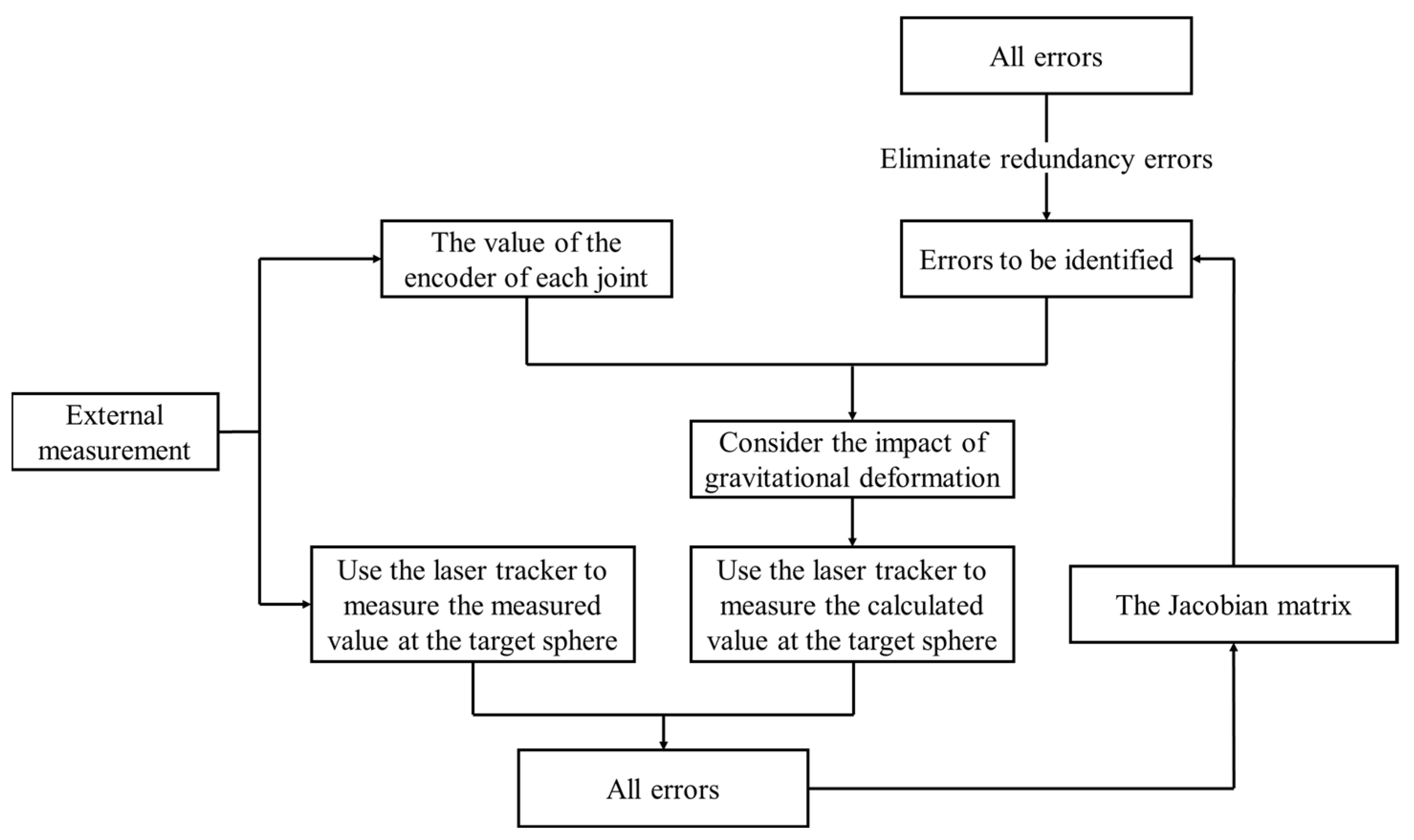
7.1. Procedures

The laser tracker model used in the experiment was Leica AT901-B, with an accuracy of (15 + 6.0 × 10⁻⁶ L^*) μm, where L^* was the measured distance, in μm. The structural parameters of the robot are listed in Table 2.

Table 2. Robot’s structural parameters.

${\mathit{a}}_2$/mm	${\mathit{a}}_3$/mm	${\mathit{a}}_4$/mm	${\mathit{d}}_1$/mm	${\mathit{d}}_2$/mm	${\mathit{d}}_6$/mm
250	1350	246	0–4000	626	1700–2300

Figure 8 presents the calibration flowchart.

Figure 8. Calibration flowchart.

As shown in Figure 9, as the terminal position of the robot could not be measured directly, a positioning plate was added to the robot terminal to mount the target sphere base of the laser tracker, and the coordinate system {e} represented the target sphere center coordinate system, that is, the tool’s coordinate system. The relationship between the tool’s coordinate system {e} and the terminal coordinate system {A7} was described by a transformation matrix A_e. Since the terminal adapter panel and laser tracker reflection sphere had high mechanical processing accuracy and were installed at the farthest distance from the robot base, the slight change in the posture had a slight effect on the final measured error. To simplify the calculation, A_e only considered the position but not the posture in this study, being was expressed as follows:

$$A_e={[\begin{array}{cccc}{p}_{ex}& p_{ey}& p_{ez}& 1\end{array}]}^T$$

(44)

Figure 9. Calibration test using a Leica laser tracker.

The tool’s coordinate system of industrial robots can be converted to the global coordinate system as

$${}^w{T}_e={}^w{T}_0{}^0{T}_1{}^1{T}_2\dots {}^6{T}_7{}^7{T}_{7\prime }{}^{7\prime }{T}_e$$

(45)

where ^wT₀ is the robot base coordinate system under the global coordinate system and ^7ʹT_e is the target spherical coordinate system under the robot terminal coordinate system. Therefore, the geometric errors in ^wT₀ and ^7ʹT_e also had to be identified during error identification. For this reason, these two errors were also included in establishing the error model to reduce the error introduced in the measurement process.

In the measurement point selection process, the points were selected from joint space. Since the robot had redundant degrees of freedom, multiple inverse solutions existed. For each joint, the two endpoints of the effective range of motion and the three joint values taken uniformly were selected, giving a total of 5⁷ = 78,125 joint input arrangements for the seven joints, which were used as candidates. They were further optimized, according to the measurement posture optimization algorithm proposed in the study [46] to obtain the final 150 sets of measured postures.

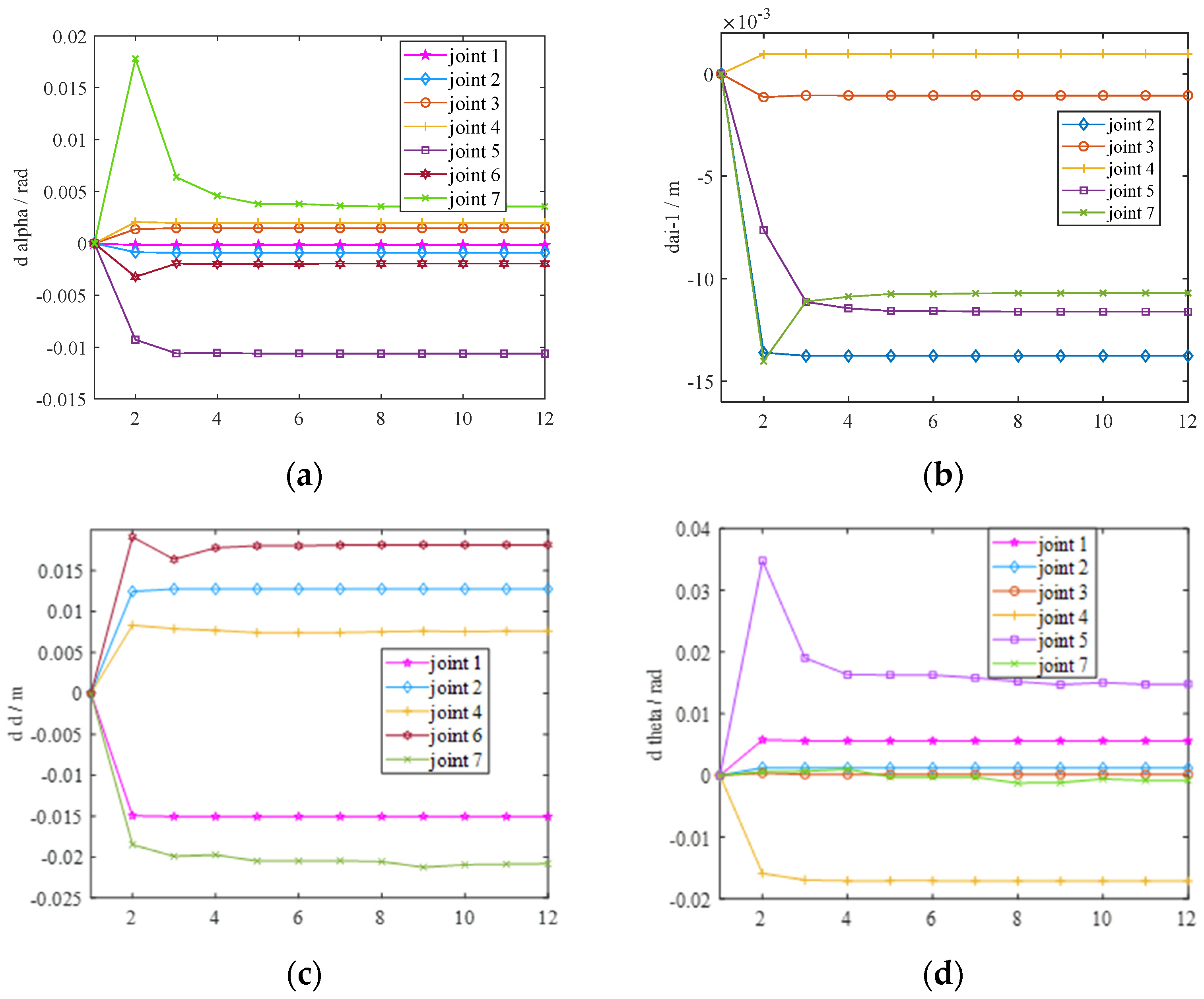
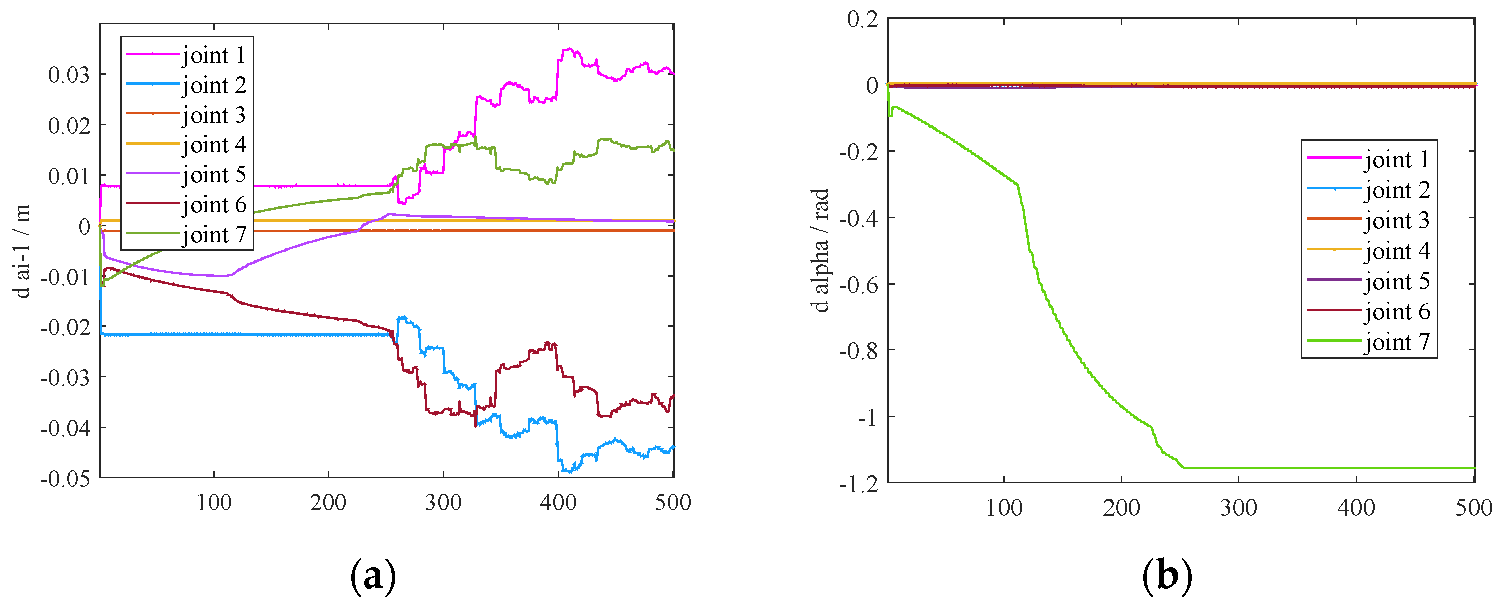
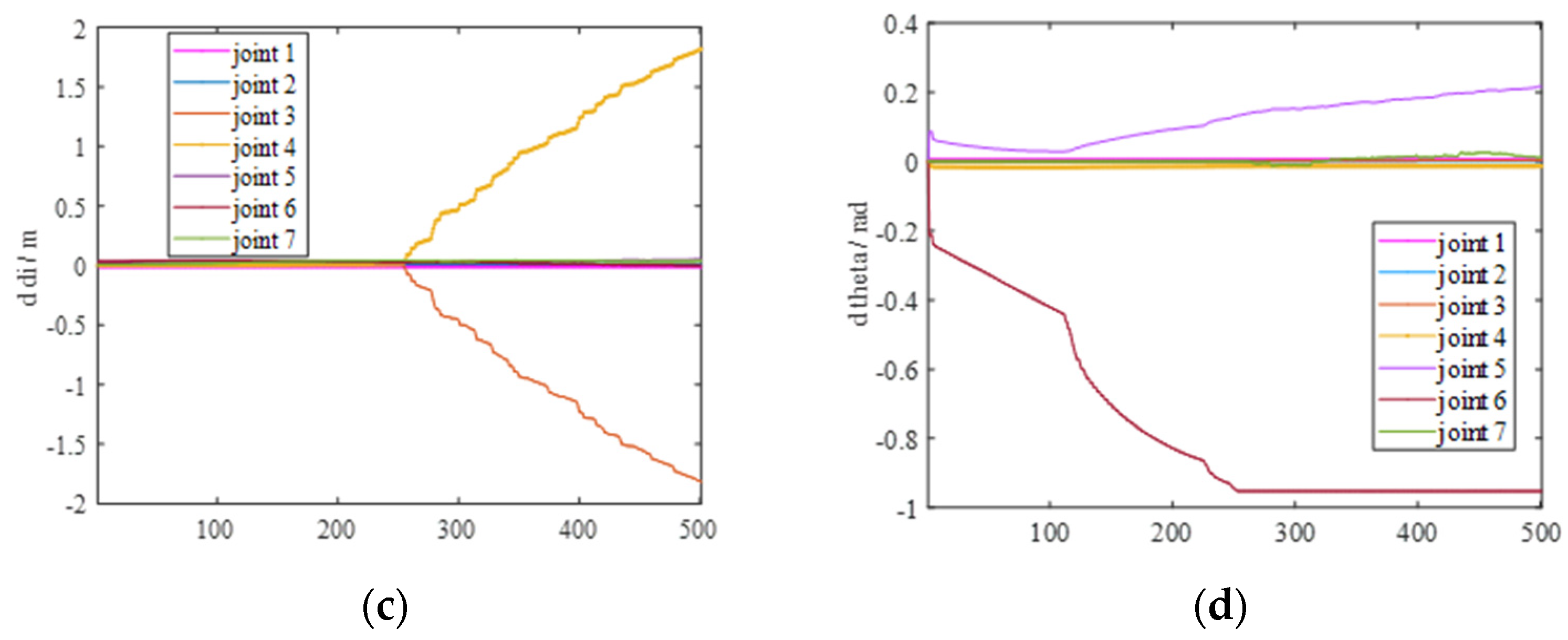
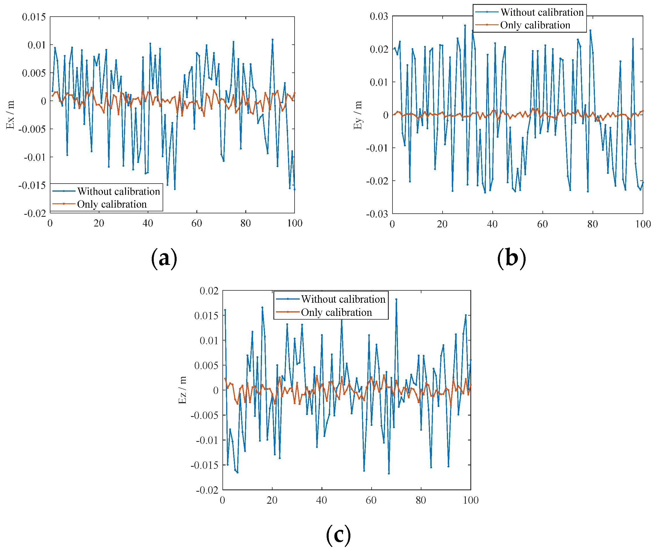
7.2. Validation of Error Elimination Effectiveness

After the elimination of redundancy error, the variation of each error item in the identification process is shownin Figure 10.

Figure 10. Identification of various parameters after the elimination of redundancy error: (a) $\delta a_{i-1}$; (b) $\delta {\alpha }_{i-1}$; (c) $\delta d_i$; (d) $\delta {\theta }_i$.

As observed, each error term can be accurately identified after eliminating redundancy error, and the identification process is stable and converges in about ten generations. As a comparison, the variation of each error item in the identification process without eliminating redundancy error is shown in Figure 11.

Figure 11. Identification of various parameters before elimination of redundancy error: (a) $\delta a_{i-1}$; (b) $\delta {\alpha }_{i-1}$; (c) $\delta d_i$; (d) $\delta {\theta }_i$.

As observed, when redundancy error is not eliminated, the identification process is unstable, there is no convergence in the error term identification, and over-fitting exists, which indicates the correctness of error term elimination.

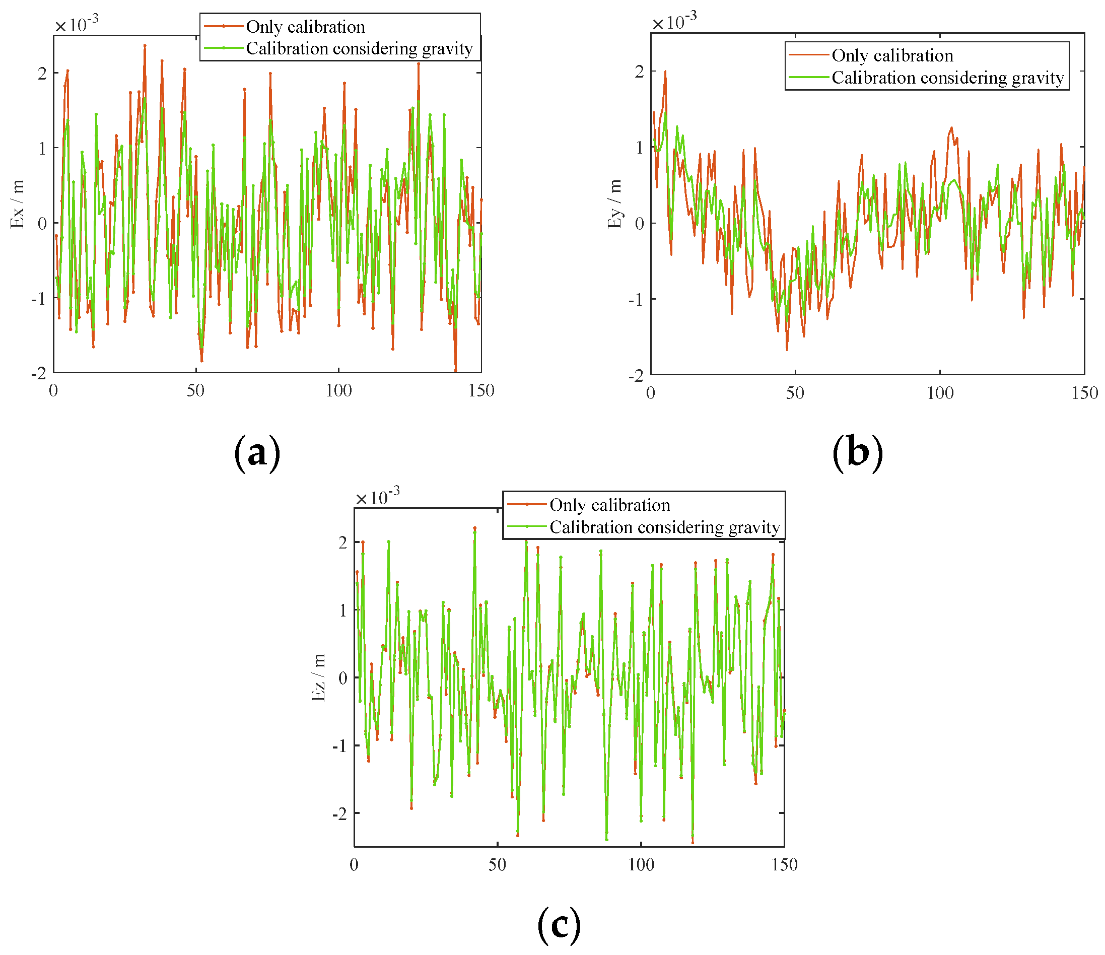
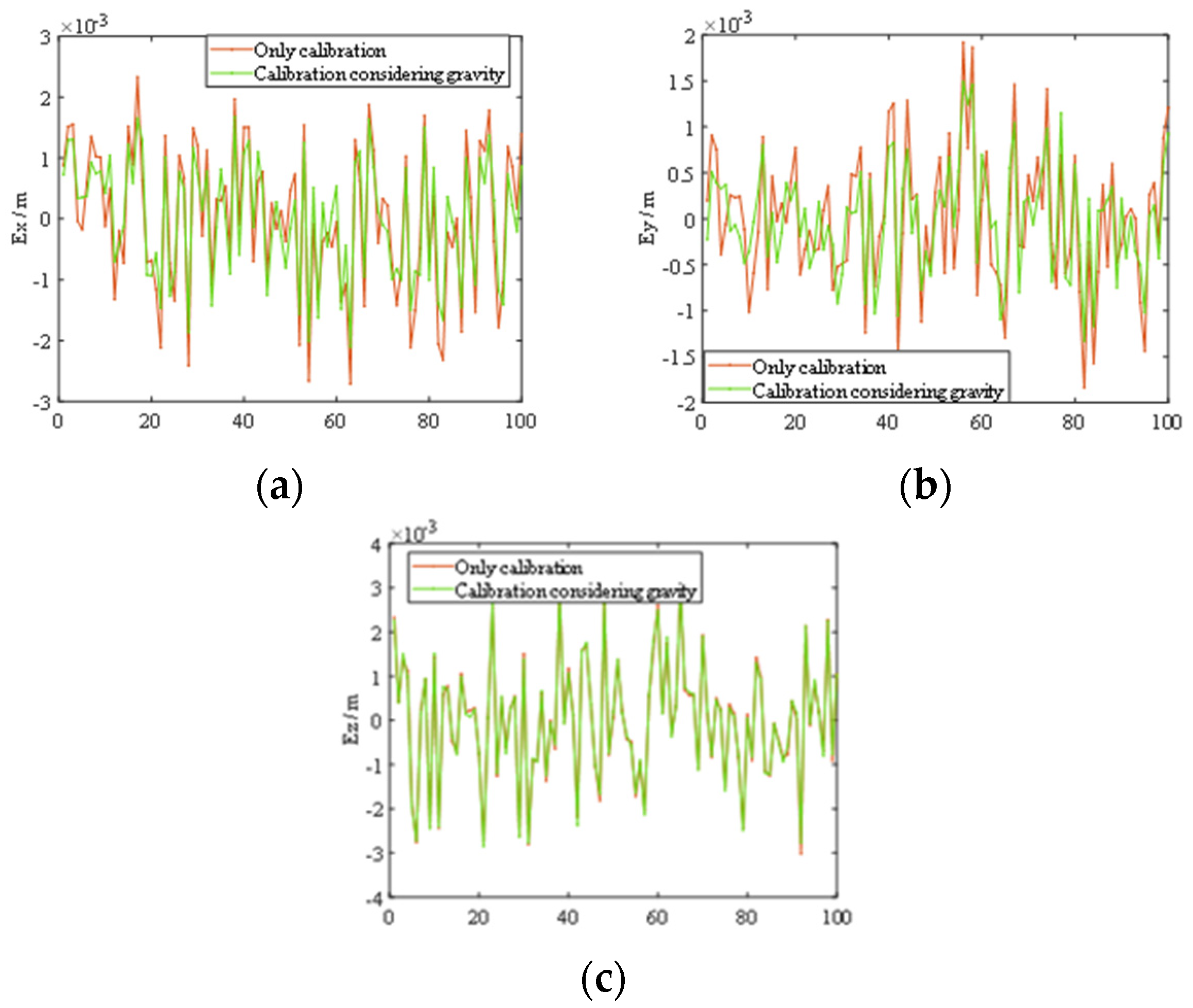
7.3. Experimental Results

One hundred fifty points were selected in the working space for measurement, and the measured results were identified, and the results obtained by using the method without calibration, the technique considering only kinematic calibration, and the calibration method considering gravity compensation were compared.

As shown in Figure 12, the errors in the X-, Y-, and Z-directions obtained by using the technique without calibration and the method considering only kinematic calibration were compared to verify the effectiveness of the proposed kinematic calibration

Figure 12. Comparison of kinematic calibration and non-calibration in the X- (a) Y- (b) and Z- (c) directions.

To illustrate the correctness of the gravity compensation model and the kinematic calibration method considering gravitational deformation, the errors in the X-, Y-, and Z-directions of the measurement points obtained by using the method considering only kinematic calibration and the kinematic calibration method considering gravitational deformation were compared in Figure 13.

Figure 13. Comparison of gravity compensation and non-compensation in the X- (a), Y- (b) and Z- (c) directions.

The errors obtained after calibration by each method are listed in Table 3.

Table 3. Maximum and mean errors obtained after calibration by various methods.

	X-Direction/m		Y-Direction/m		Z-Direction/m
	Maximum	Mean	Maximum	Mean	Maximum	Mean
Without calibration	0.0147	0.0057	0.0262	0.0144	0.0195	0.0063
Only calibration	0.0024	0.0009	0.0020	0.0006	0.0024	0.0008
Calibration considering gravity	0.0017	0.0007	0.0015	0.0004	0.0023	0.0007

For calibration alone, the error in each direction shows a reduction trend, indicating the correctness of the kinematic calibration model. Meanwhile, the error obtained by the calibration method considering gravity is smaller than that obtained by the technique considering only calibration, indicating the correctness of the proposed gravitational deformation model and the calibration method considering gravity.

After eliminating redundancy error, the error terms identified using the proposed calibration method were obtained and listed in Table 4.

Table 4. MD-H parameters of the robot after identification combined with gravity compensation.

Joint No.	$\mathit{\delta }{\mathit{a}}_{\mathit{i}-1}$/m	$\mathit{\delta }{\mathit{\alpha }}_{\mathit{i}-1}$/rad	$\mathit{\delta }{\mathit{d}}_{\mathit{i}}$/m	$\mathit{\delta }{\mathit{\theta }}_{\mathit{i}}$/rad	δβi/rad
1	-	−0.0002	−0.0151	0.0056	-
2	−0.0138	−0.0009	0.0128	0.0012	-
3	−0.0011	0.0015	-	0.0002	-
4	0.0009	0.0020	0.0076	−0.0171	0.0148
5	−0.0116	−0.0106	-	0.0148	-
6	-	−0.0019	0.0182	-	-
7	−0.0107	0.0035	−0.0208	−0.0001	-

After calibration, the measurement points’ errors were identified, as shown in Table 4. To verify the accuracy in the whole working space after calibration, some other measurement points in the entire working space were used for verification. After compensation with the identified data, 100 measurement points were used here to verify the accuracy after calibration.

For calibration only without considering gravitational deformation, the compensated error and the uncalibrated error of each measurement point were compared using the identified data, as shown in Figure 14.

Figure 14. Verification of kinematic calibration only in X- (a), Y- (b), and Z- (c) directions.

After calibration considering gravitational deformation, the compensated error, the error obtained by calibration without considering gravity, and the error obtained by only calibration of each measurement point were compared using the identified parameters, as shown in Figure 15 and tabulated in Table 5.

Figure 15. Verification of calibration considering gravity in X- (a) Y- (b), and Z- (c) directions.

Table 5. Verification of calibration considering gravity in X-, Y-, and Z-directions.

	X-Direction/m		Y-Direction/m		Z-Direction/m
	Maximum	Mean	Maximum	Mean	Maximum	Mean
Without calibration	0.0158	0.0059	0.0271	0.0139	0.0182	0.0067
Only calibration	0.0027	0.0010	0.0019	0.0006	0.0030	0.0011
Calibration considering gravity	0.0021	0.0008	0.0015	0.0005	0.0029	0.0011

8. Conclusions

A rigid-flexible coupling kinematic modeling method considering gravitational deformation was proposed for the 7-DoF spray-painting robot. The kinematic model was used to identify the robot’s geometric errors, which can simultaneously compensate for its geometric errors and gravitational deformation and improve its terminal accuracy. Firstly, the MD-H model constructed the rigid kinematic error model of the 7-DoF spraying robot. The redundancy of the geometric errors was analyzed, and the redundancy error was eliminated. Then, the stiffness matrix of each part was extracted from the finite element software by considering the part’s flexibility. The obtained matrices were joined together by MSA, thereby bringing the static stiffness matrix of the whole robot. Based on this static stiffness matrix, the effect of gravitational deformation on the terminal position of the robot was analyzed, and the MD-H rigid kinematic error model was modified to obtain a rigid-flexible coupling kinematic error model considering gravitational deformation. The regularization identification algorithm was used to identify the geometric errors. Finally, the proposed method was verified by kinematic calibration experiments, which compared the results obtained using the technique without calibration, the method considering only kinematic calibration, and the calibration method considering gravity compensation. The experimental results showed that using the rigid-flexible coupling kinematic model for calibration could achieve the highest terminal accuracy, indicating the correctness of the proposed geometric error calibration model and the gravitational deformation model. Additionally, to address the redundancy problem of the 7-DoF robot, an error compensation strategy was developed. This method can be used to improve the accuracy of large-sized 7-DoF H-Ds and is of great reference value for other mechanisms with the characteristics of the robots.

References

1. Wu, J.; Wang, J.; Wang, L.; Li, T.; You, Z. Study on the stiffness of a 5-DOF hybrid machine tool with actuation redundancy. Mech. Mach. Theory 2009, 44, 289–305. [Google Scholar] [CrossRef]
2. Wang, L.L. A brief discussion about the factors that affect the quality of aircraft parts spraying. Mod. Paint. Finish. 2014, 17, 33–35. [Google Scholar]
3. Zhai, X.W. Design and Control of Spraying Robot in Large Car Product Line. Ph.D. Thesis, Chongqing University, Chongqing, China, 2016. [Google Scholar]
4. Liu, Y.J.; Zi, B.; Wang, Z.Y.; You, W.; Zheng, L. Research Progress and Trend of Key Technology of Intelligent Spraying Robot. J. Mech. Eng. 2022, 58, 53–74. [Google Scholar]
5. Xu, P.; Cheung, C.-F.; Li, B.; Ho, L.-T.; Zhang, J.-F. Kinematics analysis of a hybrid manipulator for computer controlled ultra-precision freeform polishing. Robot. Comput. Manuf. 2017, 44, 44–56. [Google Scholar] [CrossRef]
6. Kucuk, S. Dexterous working space optimization of a new hybrid parallel robot manipulator. J. Mech. Robot. 2018, 10, 064503. [Google Scholar] [CrossRef]
7. Roth, Z.; Mooring, B.; Ravani, B. An overview of robot calibration. IEEE J. Robot. Autom. 1987, 3, 377–385. [Google Scholar] [CrossRef]
8. Judd, R.P.; Knasinski, A.B. A technique to calibrate industrial robots with experimental verification. IEEE Trans. Robot. Autom. 1990, 6, 20–30. [Google Scholar] [CrossRef]
9. Ramesh, R.; Mannan, M.A.; Poo, A.N. Error compensation in machine tools—A review: Part I: Geometric, cutting-force induced and fixture-dependent errors. Int. J. Mach. Tools Manuf. 2000, 40, 1235–1256. [Google Scholar] [CrossRef]
10. Ramesh, R.; Mannan, M.A.; Poo, A.N. Error compensation in machine tools—A review: Part II: Thermal errors. Int. J. Mach. Tools Manuf. 2000, 40, 1257–1284. [Google Scholar] [CrossRef]
11. Tan, N. Calibration for accuracy improvement of serial manipulators based on compressed sensing. Electron. Lett. 2015, 51, 820–822. [Google Scholar] [CrossRef]
12. Elatta, A.Y.; Gen, L.P.; Zhi, F.L.; Yu, D.Y.; Luo, F. An overview of robot calibration. Inf. Technol. J. 2004, 3, 74–78. [Google Scholar] [CrossRef]
13. Nubiola, A.; Bonev, I.A. Absolute calibration of an ABB IRB 1600 robot using a laser tracker. Robot. Comput. Integr. Manuf. 2013, 29, 236–245. [Google Scholar] [CrossRef]
14. Denavit, J.; Hartenberg, R.S. A Kinematic Notation for Lower-Pair Mechanisms Based on Matrices. J. Appl. Mech. 1955, 22, 215–221. [Google Scholar] [CrossRef]
15. Hayati, S.A. Robot arm geometric link parameter estimation. In The 22nd IEEE Conference on Decision and Control; IEEE: New York, NY, USA, 1983; pp. 1477–1483. [Google Scholar]
16. Stone, H.W. Kinematic Modeling, Identification, and Control of Robotic Manipulators; Springer Science and Business Media: Berlin, Germany, 2012. [Google Scholar]
17. Zhuang, H.; Roth, Z.; Hamano, F. A complete and parametrically continuous kinematic model for robot manipulators. IEEE Trans. Robot. Autom. 1992, 8, 451–463. [Google Scholar] [CrossRef]
18. Khalil, W.; Gautier, M.; Enguehard, C. Identifiable Parameters and Optimum Configurations for Robots Calibration. Robotica 1991, 9, 63–70. [Google Scholar] [CrossRef]
19. Joubair, A.; Slamani, M.; Bonev, I.A. Kinematic calibration of a five-bar planar parallel robot using all working modes. Robot. Comput. Manuf. 2013, 29, 15–25. [Google Scholar] [CrossRef]
20. Nubiola, A.; Slamani, M.; Joubair, A.; Bonev, I.A. Comparison of two calibration methods for a small industrial robot based on an optical CMM and a laser tracker. Robotica 2014, 32, 447–466. [Google Scholar] [CrossRef]
21. Renaud, P.; Andreff, N.; Lavest, J.-M.; Dhome, M. Simplifying the kinematic calibration of parallel mechanisms using vision-based metrology. IEEE Trans. Robot. 2006, 22, 12–22. [Google Scholar] [CrossRef]
22. Liu, Y.; Wu, J.; Wang, L.; Wang, J.; Wang, D.; Yu, G. Kinematic calibration of a 3-DOF parallel tool head. Ind. Robot. Int. J. Robot. Res. Appl. 2017, 44, 231–241. [Google Scholar] [CrossRef]
23. Wang, P.; Liao, Q.; Zhuang, Y.; Wei, S. Simulation and experimentation for calibration of general 7R serial robots. Robot 2006, 28, 483–487. (In Chinese) [Google Scholar]
24. Majarena, A.C.; Santolaria, J.; Samper, D.; Aguilar, J.J. Analysis and evaluation of objective functions in kinematic calibration of parallel mechanisms. Int. J. Adv. Manuf. Technol. 2013, 66, 751–761. [Google Scholar] [CrossRef]
25. Renders, J.-M.; Rossignol, E.; Becquet, M.; Hanus, R. Kinematic calibration and geometrical parameter identification for robots. IEEE Trans. Robot. Autom. 1991, 7, 721–732. [Google Scholar] [CrossRef]
26. Wang, K. Application of genetic algorithms to robot kinematics calibration. Int. J. Syst. Sci. 2009, 40, 147–153. [Google Scholar] [CrossRef]
27. Liu, Y.; Liang, B.; Li, C.; Xue, L.; Hu, S.; Jiang, Y. Calibration of a steward parallel robot using genetic algorithm. In IEEE International Conference on Mechatronics and Automation; IEEE: New York, NY, USA, 2007; pp. 2495–2500. [Google Scholar]
28. Patel, A.; Ehmann, K. Volumetric Error Analysis of a Stewart Platform-Based Machine Tool. CIRP Ann. 1997, 46, 287–290. [Google Scholar] [CrossRef]
29. Levenberg, K. A method for the solution of certain non-linear problems in least squares. Q. Appl. Math. 1944, 2, 164–168. [Google Scholar] [CrossRef]
30. Marquardt, D.W. An algorithm for least-squares estimation of nonlinear inequalities. SIAM J. Appl. Math. 1963, 11, 431–441. [Google Scholar] [CrossRef]
31. Jia, Z.Y.; Lin, S.G.; Liu, W. Measurement method of six-axis load sharing based on the Stewart platform. Measurement 2010, 43, 329–335. [Google Scholar] [CrossRef]
32. Mahboubkhah, M.; Nategh, M.J.; Khadem, S.E. A comprehensive study on the free vibration of machine tools’ hexapod table. Int. J. Adv. Manuf. Technol. 2009, 40, 1239–1251. [Google Scholar] [CrossRef]
33. Tsai, L.-W.; Joshi, S. Kinematics and Optimization of a Spatial 3-UPU Parallel Manipulator. J. Mech. Des. 2000, 122, 439–446. [Google Scholar] [CrossRef]
34. Pashkevich, A.; Chablat, D.; Wenger, P. Stiffness analysis of overconstrained parallel manipulators. Mech. Mach. Theory 2009, 44, 966–982. [Google Scholar] [CrossRef]
35. Huang, T.; Zhao, X.; Whitehouse, D. Stiffness estimation of a tripod-based parallel kinematic machine. IEEE Trans. Robot. Autom. 2002, 18, 50–58. [Google Scholar] [CrossRef]
36. Cammarata, A. Unified formulation for the stiffness analysis of spatial mechanisms. Mech. Mach. Theory 2016, 105, 272–284. [Google Scholar] [CrossRef]
37. Gosselin, C. Stiffness mapping for parallel manipulators. IEEE Trans. Robot. Autom. 1990, 6, 377–382. [Google Scholar] [CrossRef]
38. Gosselin, C.M.; Zhang, D. Stiffness analysis of parallel mechanisms using a lumped model. IEEE Trans. Robot. Autom. 2002, 17, 17–27. [Google Scholar]
39. Klimchik, A.; Pashkevich, A.; Caro, S.; Chablat, D. Stiffness Matrix of Manipulators With Passive Joints: Computational Aspects. IEEE Trans. Robot. 2012, 28, 955–958. [Google Scholar] [CrossRef]
40. Kimchi, A.; Pashkevich, A.; Chablat, D. CAD-based approach for identification of elastostatics parameters of robotic manipulators. Finite Elem. Anal. Des. 2013, 75, 19–30. [Google Scholar]
41. Mei, B.; Xie, F.G.; Liu, X.J.; Yang, C.B. Elasto-geometrical error modeling and compensation of a five-axis parallel machining robot. Precis. Eng. J. Int. Soc. Precis. Eng. Nanotechnol. 2021, 69, 48–61. [Google Scholar] [CrossRef]
42. Kimchi, A.; Bondarenko, D.; Pashkevich, A.; Briot, S.; Furet, B. Compliance error compensation in robotic-based milling. Inform. Control. Autom. Robot. 2014, 283, 197–216. [Google Scholar]
43. ASME B89.4.19-2006; Performance Evaluation of Laser-Based Spherical Coordinate Measurement Systems. ASME Press: New York, NY, USA, 2022.
44. Huang, T.; Zhao, D.; Yin, F.; Tian, W.; Chetwynd, D.G. Kinematic calibration of a 6-DoF hybrid robot by considering multicollinearity in the identification Jacobian. Mech. Mach. Theor. 2019, 131, 371–384. [Google Scholar] [CrossRef]
45. Wang, Y.; Qiu, J.; Wu, J.; Wang, J. Inverse Kinematics of a 7-DOF Spray-Painting Robot with a Telescopic Forearm. In 14th International Conference on Intelligent Robotics and Applications (ICIRA); Springer: Cham, Switzerland, 2021; pp. 666–679. [Google Scholar] [CrossRef]
46. Li, M.; Wang, L.; Yu, G.; Li, W. A new calibration method for hybrid machine tools using virtual tool center point position constraint. Measurement 2021, 181, 109582. [Google Scholar] [CrossRef]
Disclaimer/Publisher’s Note: The statements, opinions and data contained in all publications are solely those of the individual author(s) and contributor(s) and not of MDPI and/or the editor(s). MDPI and/or the editor(s) disclaim responsibility for any injury to people or property resulting from any ideas, methods, instructions or products referred to in the content.
Article Metrics
Citations
Article Access Statistics
Multiple requests from the same IP address are counted as one view.