Abstract
There have been some successful attempts to develop data-driven fault diagnostic methods in recent years. A common assumption in most studies is that the data of the source and target domains are obtained from the same sensor. Nevertheless, because electromechanical actuators may have complex motion trajectories and mechanical structures, it may not always be possible to acquire the data from a particular sensor position. When the sensor locations of electromechanical actuators are changed, the fault diagnosis problem becomes further complicated because the feature space is significantly distorted. The literature on this subject is relatively underdeveloped despite its critical importance. This paper introduces a Transformer-based end-to-end cross-sensor domain fault diagnosis method for electromechanical actuators to overcome these obstacles. An enhanced Transformer model is developed to obtain domain-stable features at various sensor locations. A convolutional embedding method is also proposed to improve the model’s ability to integrate local contextual information. Further, the joint distribution discrepancy between two sensor domains is minimized by using Joint Maximum Mean Discrepancy. Finally, the proposed method is validated using an electromechanical actuator dataset. Twenty-four transfer tasks are designed to validate cross-sensor domain adaptation fault diagnosis problems, covering all combinations of three sensor locations under different operating conditions. According to the results, the proposed method significantly outperforms the comparative method in terms of varying sensor locations.
1. Introduction
In recent years, the next generation of aerospace equipment with fly-by-wire flight control systems has increased substantially [1]. As an important type of fly-by-wire flight control actuator, Electromechanical Actuators (EMAs) are gaining increasing attention in the aerospace industry due to their many advantages, including higher reliability, lower total weight, and better maintainability. As an important safety component on a spacecraft, the EMA may fail for several reasons due to the complicated and uncertain operating environment of the spacecraft. Therefore, the safety and reliability of EMA are of critical importance, and it may lead to catastrophic consequences if EMA failures fail to be detected. Consequently, it is important to carry out fault diagnosis research on the EMA of spacecraft.
There has been increasing research in Prognostic and Health Management (PHM) in EMA over the past several years. There are two categories of approaches suggested in these studies: model-based approaches and data-driven approaches.
The model-based approach requires the development of an accurate mathematical model [2,3] to predict the input and output correlations of the EMA. Analyzing the estimated parameters of an EMA against its measurements will reveal its health state. Model-based approaches can provide insights into the operational state of individual components within an EMA, enabling faults to be identified directly from a physical perspective. Arriola et al. [4] constructed five sets of signal-based monitoring functions to detect faults based on a detailed model of EMA. Ossmann et al. [5] designed a residual filter of EMA based on a linear model, which implemented fault diagnosis by monitoring three sensors of EMA. As an advantage of using a model-based approach, the fault modes are correlated with the parameters of the model. However, this approach relies on high-fidelity models, which are often designed for specific devices. It is generally difficult or expensive to measure and calculate the model’s complete parameters outside of a laboratory.
In data-driven approaches, monitoring data and signal processing techniques are used to learn EMA fault patterns from normal and fault data. EMA fault patterns can be directly learned from sensor data when data-driven approaches are used. Data-driven approaches are becoming increasingly popular as monitoring techniques and computational power improve. Chirico et al. [6] determined the frequency domain features of vibration signals derived from EMAs using the power spectral density method, and further reduced the dimensionality of the features through principal component analysis. In the end, fault diagnosis is achieved using Bayesian classifiers. This type of traditional data-driven approach normally relies on predefined domain knowledge to extract features manually. With deep learning, it is possible to automatically learn hierarchical representations of large-scale data [7]. This is critical to fault diagnosis applications. Reddy et al. [8] employed a Deep Auto-Encoder (DAE) network to transform high-dimensional sensor data into a low-dimensional feature space to detect anomalies. Yang et al. [9] developed a sliding window enhanced EMA fault detection and isolation method using an extended Long Short-Term Memory (LSTM) model. A Convolutional Neural Network (CNN)-based EMA fault diagnosis method was presented by Riaz et al. [10]. In EMA fault diagnosis, deep learning-based approaches have achieved significant performance improvements, as they can take advantage of non-linear feature mapping and end-to-end data mining.
For a new diagnosis task, these deep neural networks always perform poorly on newly discovered target samples regardless of initial dataset training. Because there is a difference in distribution between source and target domains, this can be attributed to a variety of factors, including working conditions, mechanical characteristics, and sensor differences. [11]. To address this problem, several transfer learning techniques have been proposed that are designed to transfer fault diagnostic knowledge from one domain to another [12]. In recent years, intelligent fault diagnosis methods consisting of cross-domain adaptation and knowledge transfer can be effective for classifying fault types in varying working conditions [13,14,15,16], across different machines [17,18,19], and imbalance instances [20,21], etc.
Despite promising results from these studies, most existing research assumes data collection is conducted at the same location on each machine. It is important to note that in real-world settings, this assumption is often difficult to achieve. The source domain (training data) distribution and the target domain distribution (testing data) may change with the sensor or its location. Due to this situation, it is difficult for the knowledge acquired from the source domain to be implemented successfully in the target domain. Less attention has been given to scenarios where training and testing data are collected at different locations.
In addition, vibration signals captured by the EMA are susceptible to contamination by sensor locations as a result of its complex construction. Vibration data collected at a different location has a negative impact on both the quantity and quality of information. It may be argued that cross-sensor domain adaptation presents a challenge to fault diagnosis in EMA. In order to overcome this problem, a cross-sensor fault classifier needs to be built using learned source domain knowledge. Unfortunately, little research has been conducted on this topic. Li et al. [22] proposed a Generative Adversarial Network (GAN)-based approach for marginal domain fusion of bearing data, combined with parallel unsupervised data, to converge on conditional distribution alignments. However, GAN is not optimal for discriminative tasks, and it is sometimes limited to smaller shifts on these tasks [23]. A CNN and Maximum Mean Discrepancy (MMD) [24] were utilized by Pandhare et al. [25] for fault diagnosis across different sensor locations of a ball screw. CNN treats all data equally and lacks both pertinence and relevance, making it difficult for viewers to discover relationships between targets [26]. As of this moment, CNN has a limited ability to provide long-ranged information because of its receptive fields that are localized [27]. Though cross-sensor domain fault diagnosis is exceedingly common in real industrial scenarios, various aspects of these problems have not been adequately addressed.
A number of attention mechanisms have been successfully employed in the areas of Computer Vision (CV), Natural Language Processing (NLP), and fault detection [28,29,30]. In a recent study, Vaswani et al. [31] presented a TransformerTransformer model that relies solely on self-attention. A representation of the input data is computed based on the position of the input data. In this way, it is possible to determine global dependencies effectively and simultaneously between input and output over time. In contrast to CNN, the kernel size is not constrained, enabling a complete receptive field to be created for each time step. Contrary to Recurrent Neural Network (RNN)-based methods, the Transformer enables full parallel computation through its dot-product self-attention. Diagnostic tasks often require processing signal sequences and determining their internal correlations. Thus, a Transformer was found to have positive effects in this area [32]. The Transformer has made tremendous progress in CV and NLP. In the area of fault diagnosis, it has not yet been widely adopted.
This paper proposes an end-to-end cross-sensor domain adaptation fault diagnosis method based on enhanced Transformer and convolutional embedding. The canonical Transformer can capture long-term dependencies in parallel and makes it easy to tailor it to match different input sequence lengths. However, a canonical Transformer does not take much account of the local contexts when extracting high-level features [33]. The convolution-based input embedding method further emphasizes the contribution of local contexts to learning. Moreover, the enhanced Transformer model is developed for the EMA fault diagnosis, which takes the attention mechanism as its core and avoids the weaknesses of the CNN and LSTM models. Furthermore, Joint Maximum Mean Discrepancy (JMMD) [34] is explored for achieving feature alignment and satisfying the need for domain-invariant features. The effect of domain adversarial training on Transformer-based models is that it influences their learned representations without having much impact on their performance. It indicates that Transformer-based models are already robust across domains [35]. Therefore, adversarial learning is not considered in this study. Finally, a validation experiment is carried out on a real-world EMA fault diagnosis dataset. The experiment results indicate that the proposed method is well-suited for cross-sensor domain fault diagnosis.
The following are the main contributions of this study:
- An end-to-end cross-sensor domain fault diagnosis model is proposed. The domain adaptation is based on a source-only supervised method.
- The proposed method takes advantage of a new input embedding technique, which is investigated to incorporate the local features into the attention mechanism. An enhanced Transformer is introduced as the backbone to extract effective information from local features with an attention mechanism.
- A benchmark dataset is grouped into twenty-four transfer tasks to validate the effectiveness of the proposed method. Experimental results on EMA fault diagnosis show the excellent performance of the proposed method in terms of fault diagnosis accuracy and sensor generalization capability under different working conditions.
2. Problem Formulation
In this paper, the problem of cross-sensor domain fault diagnosis for EMAs is addressed. The proposed model will be trained on labelled data from one location sensor and transferred to unlabeled data from another location sensor. Thus, the domain of the source and the target will have different feature spaces. Labels are available in the source domain, which can be described as follows:
where denotes the source domain with labeled samples, represents the ith source domain sample of dimensions, and represents the label for the ith source domain sample.
Many existing studies based on transfer learning use semi-supervised adaptation and assume that there are a small number of available labelled samples. In this case, domain-adaptive fault diagnosis is easier to implement. It is typically not possible to access labelled target domain data in most industrial scenarios. This study focuses on unsupervised cross-sensor domain adaptation for fault diagnosis. For unsupervised learning, labelled target domain data are not available, therefore the target domain can be defined as follows:
where denotes the target domain with labeled samples and represents the ith source domain sample of dimensions.
Moreover, when testing the model, represents the label for the ith testing sample. The two label spaces in this paper are assumed to be the same, which implies:
where and denote the sets of samples from distributions and , respectively. A model that can learn transferable features is designed to bridge this discrepancy across domains, and this model will be used to classify unlabelled samples in a target domain:
where denotes the function of the fault diagnosis model and is the predicted label of .
As a result, the target risk, , is minimized by employing source domain supervision.
where denotes the model parameters.
A fault diagnostic classification model will be developed for cross-sensor domain adaptation in this study. The vibration data from sensors at one location are utilized to train a classifier that can diagnose the health status of the EMA, including normal and fault states, using data from sensors at other locations.
3. Proposed Method
This paper presents EMA fault diagnosis with cross-sensor domain adaptation using a convolutional embedding method, an enhanced Transformer model, and the JMMD algorithm. Figure 1 demonstrates the analytical pipeline for the proposed model. During the local feature extraction process, raw sensor data are mapped into local feature representations, and the feature dimension is adapted accordingly. Following this, the local features are fed into the enhanced Transformer. The architecture of the proposed enhanced Transformer is illustrated in Figure 2 and explained in Section 3.2. The total loss is calculated using the cross-entropy loss and JMMD loss. Based on the total loss, several training strategies are utilized to train the entire network. Finally, the trained model is employed to predict the health state of unlabeled EMA data samples in the target domain.
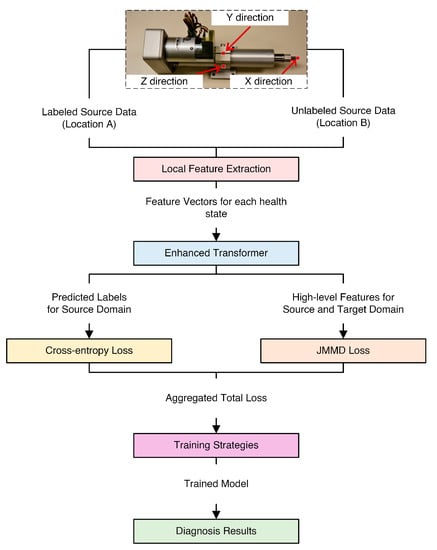
Figure 1.
Schematic of the proposed analysis pipeline.
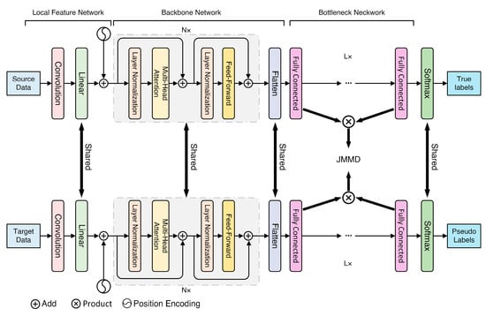
Figure 2.
Structure of the proposed model.
3.1. Local Feature Extraction
The proposed local feature network is comprised of an input embedding layer and a positional encoding layer. It maps raw sensor data into local feature representations.
Though the proposed method can learn features automatically, some data normalization steps can improve its performance. The process of data normalization is fundamental to fault diagnosis, in which input values are kept within a specific range. Z-score normalization is used to unify data magnitudes and reduce their differences.
Let denote the input sequence of the vibration signal with length . The Z-score normalization method can be implemented by:
where and are the mean and standard deviation of , respectively.
Adjacent time steps in time-series data may have stronger dependencies. In this approach, the input embedding layer consists of a convolution sublayer and a learnable linear mapping sublayer, which provides informative local features to the enhanced Transformer.
At each time step, the convolution sublayer extracts the local features, , from the input vector, , within a window, , and padding, :
By using linear mapping, the dimensions of the source and Transformer are adapted. In addition, the dropout layer is used to prevent overfitting. The linear mapping output, , is defined as:
where and are network parameters and is the dimension of the enhanced Transformer.
To account for the order of the data, a linear mapping layer is passed first, followed by a positional encoding function. As the Transformer does not contain any recurrence or convolution operations, it is necessary to inject some relative position tokens into the input to fully exploit the positioning information of the input. Sine and cosine functions with different frequencies are used to encode position.
where represents the position encoding at time step , denotes the position, and denotes the dimension. A sinusoid corresponds to each dimension of the positional encoding.
The final output of data pre-processing is denoted as :
Finally, the output of the local feature extraction is represented as .
3.2. Enhanced Transformer Based Feature Extraction
An encoder and a decoder comprise this sequence-to-sequence architecture. The encoder maps input sequences into hidden feature spaces, and the decoder uses the feature vectors to generate output sequences. The encoder may be viewed as an extractor of features in this sense. The encoder is composed of N-stacked encoder modules. Each encoder module is composed of a multi-head attention layer and a position-wise feed-forward layer. A residual connection [36] and layer normalization [37] are applied to each module. The stacked multiple encoder modules share the same structure, but their parameters differ.
This enhanced encoder introduces two major novelties: reordered layer normalization layers and using Gaussian error linear unit activation instead of standard activation.
The concept of attention can be represented by a query of an entry with key-value pairs. For input data , , , and are learnable projection matrices to generate corresponding (Query), (Key), and (Value):
where , and .
The attention of the encoder uses dot-product attention, which is defined as:
where is served as a normalization factor.
For any input vector, , the softmax function rescales the elements of the vector so that they lie in the range of [0,1] and sum to 1.
where is the th element of vector .
The Transformer is distinguished by its multi-head attention design. With multi-head attention, the input data are transformed into multiple queries, keys, and values over times. Consequently, multi-head attention enables the model to attend to information from a variety of representation subspaces at the same time. The function of multi-head attention is defined as:
where , , , and are project parameter matrices. is the number of heads.
There can only be a certain number of attention heads in a Transformer. The must be divided by without remainder. For each of these dimensions:
A layer normalization layer and a residual connector connect the input and output of the multi-head attention function after the input data, X, is passed through the multi-head attention layer.
For any vector, , the layer normalization is computed as:
where and are the mean and standard deviation of the elements in . Scale and bias vector are parameters.
A residual connector and layer normalization are used to combine the outputs of the multi-head attention layer:
where is the output of the multi-head attention layer.
In deep neural networks, residual connections are essential for alleviating information decay. However, the canonical encoder utilizes a series of layer normalization operations that non-linearly transform the state encoding. Inspired by [38], layer normalization is moved to the input streams of the submodules. Additionally, there exists a smooth gradient path, which flows directly from the output to the input without any transformation.
In this relation, the output of the multi-head attention module is changed to:
In addition, each encoder module includes a two-layer Feed-Forward Network (FFN), whose activation function is based on the Rectified Linear Unit (ReLU) [39]. For any input , ReLU is defined as:
As the term indicates, position-wise refers to applying the network to each position. The computation of the position-wise feed-forward network is defined as:
where are the weights and biases of two sub-layers, respectively.
As part of the feed-forward network, the ReLU function is used to first perform a nonlinear dimension-raising operation on the input, and then the linear layer is employed to perform a linear dimension reduction operation.
The position-wise feed-forward module connects input and output through a residual connector and a layer normalization layer:
where is the output of the position-wise feed-forward layer.
The gradient path is also smoothed by reordering the layer normalization layer. Hence, the output of the position-wise feed-forward module is changed to:
To enhance the convergence of the encoder layers, we use Gaussian error Linear Unit (GeLU) [40] activation instead of ReLU activation. An input, , and a mask, , are combined to define the GeLU function:
where is the standard Gaussian distribution function and represents the cumulative distribution function of the standard normal distribution.
where erf means the Gaussian error function.
Thus, GeLU can be formulated as:
As a continuous differentiable process, GeLU activation is more nonlinear than the ReLU activation at . Sublayer input typically follows a normal distribution, particularly when layer normalization is applied. In this setting, the probability of input becoming masked increases as decreases; therefore, using GeLU to optimize is stochastic yet depends upon input.
In this relation, the computation of the position-wise feed-forward network is changed to:
Finally, the proactive use of residual connectors, GeLU activation, and the reordering of layer normalizations contribute to a faster and more stable convergence process.
The output of the encoder is converted to a one-dimensional vector after a flatten layer. After that, the vector is mapped to higher-level features using a Fully Connected (FC) layer. As a result, high-level features are derived from the hidden features learned by the encoder. The fully connected network consists of neurons and a GeLU activation function; in addition, the dropout technique is employed to reduce overfitting.
where is the output of the last encoder module, means the function of the flatten layer, and and are the weights and biases of the fully connected layer, respectively.
Finally, the encoder maps the input data, , to high-level feature representations . In the next step, these high-level features are used for classification tasks.
3.3. Feature Transfer and Classification
A backbone and a bottleneck structure are used for transfer learning-based classification, as shown in Figure 2. In this scenario, the enhanced encoder serves as a backbone network whose output is fed into a bottleneck network. The bottleneck is used to reduce distribution discrepancy between cross-sensor domain features and to learn the transferable features. The bottleneck containing fully connected layers are transferable for domain adaptation, and their output features are handled with transfer learning strategies.
For each fully connected layer of the bottleneck, it consists of a fully connected sublayer with neurons, a GeLU activation function, and a dropout sublayer. The output features of are represented as:
where and are the weights and biases of the th fully connected layer, respectively. When , the equals .
The output of the bottleneck is passed through a softmax layer to derive a probability distribution over the output class labels. The softmax layer consists of a linear layer with neurons and a basic softmax activation function.
where is the predicted EMA health states corresponding to , and are the weights and biases of the output layer, respectively.
In other words, the function of the softmax layer is to map the transfer features to EMA health states.
The classification optimization objective includes supervision of the source domain and minimization of domain discrepancy.
In the first step, the conventional supervised machine learning paradigm is implemented, in which the categorical cross-entropy loss on the source domain is minimized.
where is the cross-entropy loss, is the indicator function, and is the number of EMA health states.
The total loss of the classifier model can be formulated as:
where is the trade-off factor and is the partial loss to close the discrepancy between source and target domains.
In a classifier model, the cross-entropy loss function is effective if the training and testing data come from the same sensor location. The domain shift is aligned by upgrading the optimization method by including JMMD in the loss function.
JMMD is used for addressing the domain shift created by joint distributions. The difference in the joint distribution can be expressed as:
JMMD measures the discrepancy between two joint distributions, and , based on their Hilbert space embeddings. The joint distribution discrepancy between the source and target domains is calculated as follows:
where denotes the mathematical expectation, is reproducing kernel Hilbert space (RKHS), is the mapping to RKHS, represents the number of fully connected layers of the bottleneck, is the feature map in the tensor product Hilbert space, and and are the source domain features and target domain features in the th fully connected layers of the bottleneck, respectively.
can be formulated as:
To address the domain shift issue, the cross-entropy loss and the discrepancy loss are integrated into the optimization objective. In this way, the total loss can be calculated as follows:
During network training, the parameters can be upgraded at each epoch as follows:
where denotes the learning rate.
4. Experiment Study
4.1. Dataset Description
To verify the effectiveness of the proposed method for cross-sensor domain fault diagnosis of EMA, we use the Flyable Electromechanical Actuator (FLEA) dataset provided by the National Aeronautics and Space Administration (NASA), Ames Research Center [41]. As shown in Figure 3, the FLEA contains three different actuators:
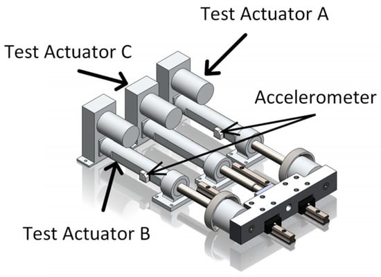
Figure 3.
FLEA System.
- Actuator A—Fault-injected test actuator;
- Actuator B—The nominal test actuator;
- Actuator C—Load actuator.
By switching the load actuator from actuator B to actuator A, FLEA enables fault injection without changing the operating state of the EMA system.
Additionally, two nut accelerometers were attached to actuators A and B. The accelerometers were used to collect vibration data at a sampling frequency of 20 kHz. In Figure 4, it is shown that the accelerometer was in three different directions (X is in line with the actuator motion, Y is vertical, and Z is horizontal).
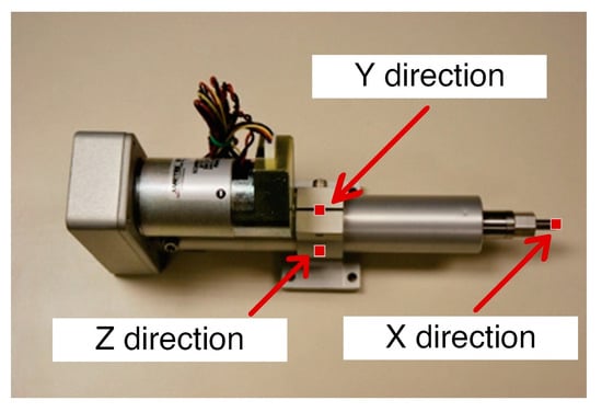
Figure 4.
Directions of the accelerometer.
In this study, there were four classes of data: the normal state, ball screw return channel jam, screw surface spall, and motor failure. Detailed information on the dataset is provided in Table 1.

Table 1.
Description of the case study dataset.
The acceleration signal of the four states from the three directions in experiment 3 is taken as an example in Figure 5, respectively. The signals in the three directions have different amplitudes and shapes.
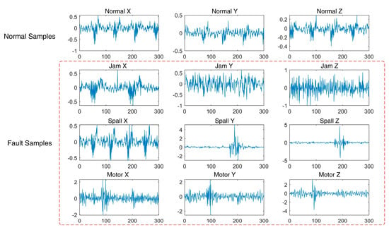
Figure 5.
Acceleration signal. Jam is the ball screw return channel jam. Spall means screw surface spall. Motor denotes the motor failure.
4.2. Transfer Task Description
In practice, EMAs work under a variety of conditions and handle complex transmission chains. Therefore, the transfer tasks should include a variety of scenarios that vary in the driving waveforms, load profiles, and output directions.
Four experiments were conducted, as described in Table 1, to examine the effects of varying working conditions upon transfer task performance. Only the data from actuator A was used in the source and target domains. EMA fault diagnosis is performed by utilizing all possible sensor location combinations under the four working conditions. The detailed information for the six-class cross-sensor fault diagnosis tasks is presented in Table 2.

Table 2.
Transfer tasks.
Generally, location X is more sensitive to faults than locations Y and Z. However, locations Y and Z are more convenient for installing sensors than location X.
Tasks T1 and T2 are aimed at determining the efficiency of the feature transfer process from fault-critical sensor locations (location X) to locations that can be implemented easily (locations Y and Z).
Tasks T3 and T4 evaluate the transferability from locations Y and Z to location X to demonstrate the effectiveness of the transferability from signals located at locations with less health information to those located at locations with more health information.
Tasks T5 and T6 examine the transferability of measurement axes between the Y and Z locations to analyze different health information.
In addition to each task, four subtasks were designed for a thorough evaluation under different working conditions.
4.3. Compared Approaches
To validate the effectiveness of the proposed method, four different approaches are examined in comparison, sharing a similar experimental setting as the proposed method.
(1) 1D-CNN (CNN)
The 1D CNN method can be used to establish a baseline for fault diagnosis. Using the CNN results, a baseline could be established for detecting faults across sensor domains without the need for transfer learning.
(2) Basic-Transformer (BT)
The Basic-Transformer method is the traditional encoder of Transformer that has not been improved, and it only uses as the loss function.
(3) Enhanced-Transformer (ET)
The proposed enhanced encoder is trained based on the source domain, which implies that source supervision is the only optimization objective. After that, the enhanced encoder is employed to recognize the health state represented by the EMA data of the target domain
(4) CNN-JMMD (CJ)
This method is composed of CNN and JMMD. The JMMD is used to reduce the distribution difference in the bottleneck.
(5) Enhanced-Transformer-JMMD (ETJ)
This method is a joint usage of the local feature extraction network, the enhanced encoder model, and JMMD. It indicates that and have been considered for optimization.
4.4. Model Parameters
Data are fed into the proposed network as they are in the time domain and have a dimension of 128. To compare network performance, the CNN and the enhanced encoder were set to have similar dimensions and layers. Table 3 summarizes the architecture and parameters of the Encoder-JMMD. The architecture and parameters of the CNN are shown in Table 4. The bottleneck of the encoder-JMMD is shared by the CNN-JMMD.

Table 3.
Parameters of Encoder-JMMD.

Table 4.
Backbone Parameters of CNN.
4.5. Training Strategies
Raw vibration data collected from the FLEA is divided into three sets. The first set is the labelled data from the source domain. The second dataset, composed of 80% of the unlabeled data from the target domain, is used for model training to align the domains. The rest of the unlabeled data constitute the third dataset and are used to evaluate the trained model. It is important to note that there is no overlap between the second and third datasets.
To initialize the network for model training, the Xavier normal initializer is employed. In addition to the back-propagation method, the Adam optimization method is used for updating all parameters. The fault diagnosis model is trained for 150 epochs.
It is necessary to predict pseudo labels for the target domain to perform the JMMD calculation. However, the pseudo labels predicted in the initial iteration may not be accurate to the target domains. Hence, the model is trained with source samples in the previous 50 epochs, meaning the pseudo labels can be predicted after 50 epochs. Subsequently, transfer learning strategies are employed. A minibatch Adam optimizer and a step learning strategy are employed as a learning rate annealing method. The learning rate was set to 0.001 at the beginning of the training. To avoid obtaining a local optimum, the learning rate is reduced to 0.0001 after 100 training cycles.
Furthermore, a progressive training method is used to increase the trade-off parameter from 0 to 1:
where is the training epochs that change from 50 to 150 [42].
5. Results and Discussion
5.1. Overall Results
The statistical results of the twenty-four tasks are shown in Table 5.

Table 5.
The diagnosis accuracy of different tasks corresponding to the different methods.
The typical 1D CNN method has an average accuracy of less than 70%, which makes it difficult to diagnose faults with multiple tasks. As a result, cross-sensor domain adaptation poses significant challenges and cannot be directly addressed by existing deep learning approaches.
The basic Transformer improves average accuracy over the 1D CNN by 11.15 percent, which is a result of better model characterization.
The enhanced Transformer provides a 5.12% improvement in average accuracy over the basic Transformer. The standard deviation of the basic Transformer is greater than that of the enhanced Transformer, indicating that the proposed model is more stable. This suggests that the proposed model has the potential to be generalized and to diagnose faults effectively.
When combined with JMMD, the CNN method provides an average diagnosis accuracy of over 90%. The average accuracy of the enhanced Transformer-JMMD is even higher than 97%. By aligning conditional data, transfer strategies achieve significantly better diagnosis results. This is caused by the fact that vibration data were collected from two different locations with vast differences in distribution.
Among these five methods, the proposed enhanced Transformer-JMMD method is the most accurate in terms of both mean and standard deviation of accuracy for all tasks. Furthermore, all the methods have great difficulties in performing the transfer tasks specified in T1 and T2, which are designed to determine whether a method can transfer knowledge from an optimal to a suboptimal sensor location. Fortunately, the average accuracy of T1 and T2 is greatly improved by the method proposed in this paper.
5.2. Visualization
A histogram is depicted in Figure 6 to provide a more intuitive visual representation of test accuracy.
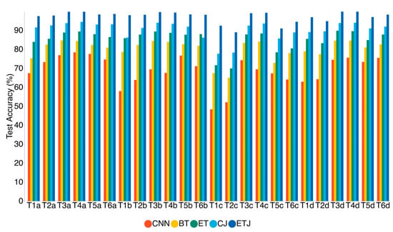
Figure 6.
Diagnosis accuracy of Table 5 in a histogram.
The proposed method demonstrates significantly higher accuracy compared to other methods. Particularly, the proposed method exhibits better results than the commonly used CJ algorithm in each task. It appears that the proposed method is beneficial in dealing with cross-sensor problems.
A t-distributed Stochastic Neighbor Embedding (t-SNE) approach is also used in Figure 1 to display high-level features for tasks T3d and T1c. Because there were too many test samples, 200 samples were randomly selected for feature visualization.
A comparison of the CNN and ETJ methods in task T3d is presented in Figure 7a,b. With the CNN method, even for the simplest tasks, there are significant discrepancies between the source and target domains. Considering the same health state of different domains, the data are projected into different places. Therefore, the CNN method acquires a low diagnostic accuracy in the target domain. Based on this finding, it appears that well-established approaches cannot be used directly to generalize the knowledge learned under source supervision into target domains. Figure 7b demonstrates that the data for the two domains under the same health state are accurately mapped into close high-level feature spaces using the proposed method. Most features with the same label across the two domains can be clustered together, and only a few samples were incorrectly classified.
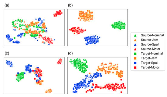
Figure 7.
Visualizations of the high-level features. (a) Task T3d | CNN; (b) Task T3d | ETJ; (c) Task T1c | CJ; (d) Task T1c | ETJ.
The CJ and ETJ methods were compared for the most challenging task, T1c. In Figure 7c,d, the visualization results of the CJ and ETJ for task T1c are presented. Although JMMD minimizes the discrepancy between the source and target domain distributions, the CJ method is still generally inefficient, with a high rate of misclassification. Utilizing the enhanced Transformer in the same task significantly improves the performance. The three fault classes still exhibit domain gaps, even after a satisfactory clustering phenomenon has been achieved in the four classes. Consequently, negative testing performances are seen for all three classes, as illustrated by Figure 7d. Comparatively, the other methods are significantly less capable of achieving cross-sensor domain adaptation for task T1c, resulting in very low numerical test accuracy, as shown in Table 5.
Figure 8 illustrates the confusion matrices corresponding to tasks T3d and T1c. This figure compares the predicted results with the ground truth for different tasks. In Figure 8b the proposed method can achieve high diagnostic accuracies in all health states with few misclassifications. Figure 8d illustrates how the proposed model can distinguish most health states for task T1c. The normal state is likely to have the most similar representations, making it easier to align the distributions and, in turn, results in optimal performance. The proposed method is also significantly more accurate than the CJ method in classifying faults.
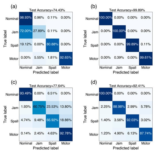
Figure 8.
Confusion matrices. (a) Task T3d | CNN; (b) Task T3d | ETJ; (c) Task T1c | CJ; (d) Task T1c | ETJ.
6. Conclusions
In this paper, we propose an end-to-end cross-sensor domain fault diagnosis method for electromechanical actuators. An enhanced Transformer model is designed to obtain stable features. The enhanced Transformer reorders the layer normalization layers and replaces the standard ReLU activation with GeLU activation. With these improvements, the proposed model offers more stable optimization and greater robustness than the canonical architecture. Furthermore, in addition to the enhanced Transformer’s ability to obtain global information, we propose a convolution-based embedding technique to improve the model’s ability to incorporate local contexts. The Joint Maximum Mean Discrepancy metric is employed in conjunction with the enhanced Transformer to optimize the distribution of the source and target domains corresponding to the various sensor locations. A real-world dataset of electromechanical actuators with three sensor locations and four health states is used to validate the proposed method. As demonstrated by the experimental results, the proposed method achieves outstanding results for a variety of sensor position transfer tasks under different working conditions. Therefore, the method proposed in this paper can effectively solve the problem of cross-sensor domain fault diagnosis of electromechanical actuators, which is a consequence of their complex construction, driving waveform, and load profile. In the future, we will research more EMA fault classes and more complex sensor locations.
Author Contributions
Conceptualization, Z.C.; methodology, Z.C.; software, Z.C.; validation, Z.C. and C.H.; formal analysis, Z.C.; investigation, Z.C.; resources, Z.C.; data curation, Z.C. and C.H.; writing—original draft preparation, Z.C.; writing—review and editing, Z.C.; visualization, Z.C.; supervision, Z.C.; project administration, Z.C.; funding acquisition, Z.C. All authors have read and agreed to the published version of the manuscript.
Funding
This research received no external funding.
Conflicts of Interest
The authors declare no conflict of interest.
References
- Mazzoleni, M.; Di Rito, G.; Previdi, F. Electro-Mechanical Actuators for the More Electric Aircraft; Springer: Cham, Switzerland, 2021; ISBN 3-030-61798-X. [Google Scholar]
- Garza, P.; Perinpanayagam, S.; Aslam, S.; Wileman, A. Qualitative Validation Approach Using Digital Model for the Health Management of Electromechanical Actuators. Appl. Sci. 2020, 10, 7809. [Google Scholar] [CrossRef]
- Quattrocchi, G.; Berri, P.C.; Dalla Vedova, M.D.L.; Maggiore, P. An Improved Fault Identification Method for Electromechanical Actuators. Aerospace 2022, 9, 341. [Google Scholar] [CrossRef]
- Arriola, D.; Thielecke, F. Model-Based Design and Experimental Verification of a Monitoring Concept for an Active-Active Electromechanical Aileron Actuation System. Mech. Syst. Signal Process. 2017, 94, 322–345. [Google Scholar] [CrossRef]
- Ossmann, D.; van der Linden, F.L.J. Advanced Sensor Fault Detection and Isolation for Electro-Mechanical Flight Actuators. In Proceedings of the 2015 NASA/ESA Conference on Adaptive Hardware and Systems (AHS), Montreal, QC, Canada, 15–18 June 2015; pp. 1–8. [Google Scholar]
- Chirico, A.J., III; Kolodziej, J.R. A Data-Driven Methodology for Fault Detection in Electromechanical Actuators. J. Dyn. Syst. Meas. Control 2014, 136, 041025. [Google Scholar] [CrossRef]
- Rezaeianjouybari, B.; Shang, Y. Deep Learning for Prognostics and Health Management: State of the Art, Challenges, and Opportunities. Measurement 2020, 163, 107929. [Google Scholar] [CrossRef]
- Reddy, K.K.; Sarkar, S.; Venugopalan, V.; Giering, M. Anomaly Detection and Fault Disambiguation in Large Flight Data: A Multi-Modal Deep Auto-Encoder Approach. In Proceedings of the Annual Conference of the PHM Society, Denver, CO, USA, 3–6 October 2016; Volume 8. [Google Scholar] [CrossRef]
- Yang, J.; Guo, Y.; Zhao, W. Long Short-Term Memory Neural Network Based Fault Detection and Isolation for Electro-Mechanical Actuators. Neurocomputing 2019, 360, 85–96. [Google Scholar] [CrossRef]
- Riaz, N.; Shah, S.I.A.; Rehman, F.; Gilani, S.O.; Udin, E. A Novel 2-D Current Signal-Based Residual Learning with Optimized Softmax to Identify Faults in Ball Screw Actuators. IEEE Access 2020, 8, 115299–115313. [Google Scholar] [CrossRef]
- Li, W.; Huang, R.; Li, J.; Liao, Y.; Chen, Z.; He, G.; Yan, R.; Gryllias, K. A Perspective Survey on Deep Transfer Learning for Fault Diagnosis in Industrial Scenarios: Theories, Applications and Challenges. Mech. Syst. Signal Process. 2022, 167, 108487. [Google Scholar] [CrossRef]
- Zhao, Z.; Zhang, Q.; Yu, X.; Sun, C.; Wang, S.; Yan, R.; Chen, X. Applications of Unsupervised Deep Transfer Learning to Intelligent Fault Diagnosis: A Survey and Comparative Study. IEEE Trans. Instrum. Meas. 2021, 70, 3525828. [Google Scholar] [CrossRef]
- Wang, J.; Zhang, Y.; Luo, C.; Miao, Q. Deep Learning Domain Adaptation for Electro-Mechanical Actuator Fault Diagnosis under Variable Driving Waveforms. IEEE Sens. J. 2022, 22, 10783–10793. [Google Scholar] [CrossRef]
- Zhang, Z.; Chen, H.; Li, S.; An, Z. Unsupervised Domain Adaptation via Enhanced Transfer Joint Matching for Bearing Fault Diagnosis. Measurement 2020, 165, 108071. [Google Scholar] [CrossRef]
- Shao, S.; McAleer, S.; Yan, R.; Baldi, P. Highly Accurate Machine Fault Diagnosis Using Deep Transfer Learning. IEEE Trans. Ind. Inform. 2019, 15, 2446–2455. [Google Scholar] [CrossRef]
- Zhou, Y.; Kumar, A.; Parkash, C.; Vashishtha, G.; Tang, H.; Xiang, J. A Novel Entropy-Based Sparsity Measure for Prognosis of Bearing Defects and Development of a Sparsogram to Select Sensitive Filtering Band of an Axial Piston Pump. Measurement 2022, 203, 111997. [Google Scholar] [CrossRef]
- Yang, B.; Lei, Y.; Xu, S.; Lee, C.-G. An Optimal Transport-Embedded Similarity Measure for Diagnostic Knowledge Transferability Analytics across Machines. IEEE Trans. Ind. Electron. 2022, 69, 7372–7382. [Google Scholar] [CrossRef]
- Zhiyi, H.; Haidong, S.; Lin, J.; Junsheng, C.; Yu, Y. Transfer Fault Diagnosis of Bearing Installed in Different Machines Using Enhanced Deep Auto-Encoder. Measurement 2020, 152, 107393. [Google Scholar] [CrossRef]
- Li, X.; Jiang, H.; Wang, R.; Niu, M. Rolling Bearing Fault Diagnosis Using Optimal Ensemble Deep Transfer Network. Knowl. Based Syst. 2021, 213, 106695. [Google Scholar] [CrossRef]
- Zareapoor, M.; Shamsolmoali, P.; Yang, J. Oversampling Adversarial Network for Class-Imbalanced Fault Diagnosis. Mech. Syst. Signal Process. 2021, 149, 107175. [Google Scholar] [CrossRef]
- Zou, L.; Li, Y.; Xu, F. An Adversarial Denoising Convolutional Neural Network for Fault Diagnosis of Rotating Machinery under Noisy Environment and Limited Sample Size Case. Neurocomputing 2020, 407, 105–120. [Google Scholar] [CrossRef]
- Li, X.; Zhang, W.; Xu, N.-X.; Ding, Q. Deep Learning-Based Machinery Fault Diagnostics with Domain Adaptation across Sensors at Different Places. IEEE Trans. Ind. Electron. 2020, 67, 6785–6794. [Google Scholar] [CrossRef]
- Tzeng, E.; Hoffman, J.; Saenko, K.; Darrell, T. Adversarial Discriminative Domain Adaptation. In Proceedings of the 2017 IEEE Conference on Computer Vision and Pattern Recognition (CVPR), Honolulu, HI, USA, 21–26 July 2017; pp. 2962–2971. [Google Scholar]
- Long, M.; Cao, Y.; Wang, J.; Jordan, M. Learning Transferable Features with Deep Adaptation Networks. In Proceedings of the 32nd International Conference on Machine Learning, ICML’15, Lille, France, 6–11 July 2015; Bach, F., Blei, D., Eds.; Volume 37, pp. 97–105. [Google Scholar]
- Pandhare, V.; Li, X.; Miller, M.; Jia, X.; Lee, J. Intelligent Diagnostics for Ball Screw Fault through Indirect Sensing Using Deep Domain Adaptation. IEEE Trans. Instrum. Meas. 2021, 70, 2504211. [Google Scholar] [CrossRef]
- Wu, B.; Xu, C.; Dai, X.; Wan, A.; Zhang, P.; Tomizuka, M.; Keutzer, K.; Vajda, P. Visual Transformers: Token-Based Image Representation and Processing for Computer Vision. CoRR 2020, arXiv:2006.03677v4. [Google Scholar]
- Gulati, A.; Qin, J.; Chiu, C.-C.; Parmar, N.; Zhang, Y.; Yu, J.; Han, W.; Wang, S.; Zhang, Z.; Wu, Y.; et al. Conformer: Convolution-Augmented Transformer for Speech Recognition. In Proceedings of the Interspeech 2020, Shanghai, China, 25–29 October 2020; pp. 5036–5040. [Google Scholar]
- Xu, Z.; Li, C.; Yang, Y. Fault Diagnosis of Rolling Bearings Using an Improved Multi-Scale Convolutional Neural Network with Feature Attention Mechanism. ISA Trans. 2021, 110, 379–393. [Google Scholar] [CrossRef] [PubMed]
- Li, X.; Zhang, W.; Ding, Q. Understanding and Improving Deep Learning-Based Rolling Bearing Fault Diagnosis with Attention Mechanism. Signal Process. 2019, 161, 136–154. [Google Scholar] [CrossRef]
- Zhang, X.; He, C.; Lu, Y.; Chen, B.; Zhu, L.; Zhang, L. Fault Diagnosis for Small Samples Based on Attention Mechanism. Measurement 2022, 187, 110242. [Google Scholar] [CrossRef]
- Vaswani, A.; Shazeer, N.; Parmar, N.; Uszkoreit, J.; Jones, L.; Gomez, A.N.; Kaiser, Ł.; Polosukhin, I. Attention Is All You Need. In Advances in Neural Information Processing Systems 30; Curran Associates Inc.: Red Hook, NY, USA, 2017; pp. 5998–6008. [Google Scholar]
- Ding, Y.; Jia, M.; Miao, Q.; Cao, Y. A Novel Time-Frequency Transformer Based on Self-Attention Mechanism and Its Application in Fault Diagnosis of Rolling Bearings. Mech. Syst. Signal Process. 2022, 168, 108616. [Google Scholar] [CrossRef]
- Li, S.; Jin, X.; Xuan, Y.; Zhou, X.; Chen, W.; Wang, Y.-X.; Yan, X. Enhancing the Locality and Breaking the Memory Bottleneck of Transformer on Time Series Forecasting. In Advances in Neural Information Processing Systems; Wallach, H., Larochelle, H., Beygelzimer, A., d’Alché-Buc, F., Fox, E., Garnett, R., Eds.; Curran Associates, Inc.: Red Hook, NY, USA, 2019; Volume 32. [Google Scholar]
- Long, M.; Zhu, H.; Wang, J.; Jordan, M.I. Deep Transfer Learning with Joint Adaptation Networks. In Proceedings of the 34th International Conference on Machine Learning, Sydney, Australia, 6–11 August 2017; Precup, D., Teh, Y.W., Eds.; Volume 70, pp. 2208–2217. [Google Scholar]
- Wright, D.; Augenstein, I. Transformer Based Multi-Source Domain Adaptation. arXiv 2020. [Google Scholar] [CrossRef]
- He, K.; Zhang, X.; Ren, S.; Sun, J. Deep Residual Learning for Image Recognition. In Proceedings of the IEEE Conference on Computer Vision and Pattern Recognition (CVPR), Las Vegas, NV, USA, 27–30 June 2016; pp. 770–778. [Google Scholar]
- Ba, J.L.; Kiros, J.R.; Hinton, G.E. Layer Normalization. arXiv 2016. [Google Scholar] [CrossRef]
- Xiong, R.; Yang, Y.; He, D.; Zheng, K.; Zheng, S.; Xing, C.; Zhang, H.; Lan, Y.; Wang, L.; Liu, T. On Layer Normalization in the Transformer Architecture. In Proceedings of the 37th International Conference on Machine Learning, ICML’20, Vienna, Austria, 12–18 July 2020; Daumé, H., III, Singh, A., Eds.; Volume 119, pp. 10524–10533. [Google Scholar]
- Nair, V.; Hinton, G.E. Rectified Linear Units Improve Restricted Boltzmann Machines. In ICML’20, Proceedings of the 27th International Conference on International Conference on Machine Learning, Haifa, Israel, 21–24 June 2010; Omnipress: Madison, WI, USA, 2010; pp. 807–814. [Google Scholar]
- Hendrycks, D.; Gimpel, K. Gaussian Error Linear Units (Gelus). arXiv 2016, arXiv:1606.08415. [Google Scholar]
- Balaban, E.; Saxena, A.; Narasimhan, S.; Roychoudhury, I.; Koopmans, M.; Ott, C.; Goebel, K. Prognostic Health-Management System Development for Electromechanical Actuators. J. Aerosp. Inf. Syst. 2015, 12, 329–344. [Google Scholar] [CrossRef]
- Long, M.; Cao, Z.; Wang, J.; Jordan, M.I. Conditional Adversarial Domain Adaptation. In Advances in Neural Information Processing Systems 31; Curran Associates Inc.: Red Hook, NY, USA, 2018. [Google Scholar] [CrossRef]
Disclaimer/Publisher’s Note: The statements, opinions and data contained in all publications are solely those of the individual author(s) and contributor(s) and not of MDPI and/or the editor(s). MDPI and/or the editor(s) disclaim responsibility for any injury to people or property resulting from any ideas, methods, instructions or products referred to in the content. |
© 2023 by the authors. Licensee MDPI, Basel, Switzerland. This article is an open access article distributed under the terms and conditions of the Creative Commons Attribution (CC BY) license (https://creativecommons.org/licenses/by/4.0/).