Article

Multi-Objective Optimization and Optimal Airfoil Blade Selection for a Small Horizontal-Axis Wind Turbine (HAWT) for Application in Regions with Various Wind Potential

by
Vahid Akbari
1,
Mohammad Naghashzadegan
2,*,
Ramin Kouhikamali
2,
Farhad Afsharpanah
3 and
Wahiba Yaïci
4
1
Department of Mechanical Engineering, University Campus 2, University of Guilan, Rasht 41996, Iran
2
Department of Mechanical Engineering, University of Guilan, Rasht 41996, Iran
3
Department of Mechanical Engineering, Babol Noshirvani University of Technology, Babol 47148, Iran
4
CanmetENERGY Research Centre, Natural Resources Canada, Ottawa, ON K1A 1M1, Canada
*
Author to whom correspondence should be addressed.
Machines 2022, 10(8), 687; https://doi.org/10.3390/machines10080687
Submission received: 23 June 2022 / Revised: 5 August 2022 / Accepted: 12 August 2022 / Published: 13 August 2022
(This article belongs to the Special Issue Wind Turbine Technologies)

Abstract

:
The type of airfoil with small wind turbine blades should be selected based on the wind potential of the area in which the turbine is used. In this study, 10 low Reynolds number airfoils, namely, BW-3, E387, FX 63-137, S822, S834, SD7062, SG6040, SG6043, SG6051, and USNPS4, were selected and their performance was evaluated in a 1 kW wind turbine in terms of the power coefficient and also the startup time, by performing a multi-objective optimization study. The blade element momentum technique was utilized to perform the calculations of the power coefficient and startup time and the differential evolution algorithm was employed to carry out the optimization. The results reveal that the type of airfoil used in the turbine blade, aside from the aerodynamic performance, completely affects the turbine startup performance. The SG6043 airfoil has the highest power coefficient and the BW-3 airfoil presents the shortest startup time. The high lift-to-drag ratio of the SG6043 airfoil and the low inertia of the turbine blades fitted with the BW-3 airfoil make them suitable for operation in windy regions and areas with low wind speeds, respectively.

1. Introduction

In today’s developed world, energy is a cardinal factor for the sustainable development and economic growth of a country [1], and, in recent years, continuous access to inexpensive and reliable energy has become an essential right for humanity [2]. However, the rise in energy demand and dependence on fossil fuels has led to energy crises, declining resources, and environmental pollution [3]. Although optimizing energy systems [4,5] and employing energy storage devices [6] are considered by scholars, the use of renewable energy sources [7] is one of the most effective solutions to cope with these difficulties. Among renewable energy sources, wind energy is the most common and sustainable type of energy and, currently, the application of this free energy source is being considered more than ever [8]. Harnessing wind energy and converting it to electrical power is carried out with the aid of wind turbines.
The shape of a wind turbine blade has a substantial role in its performance and should be determined according to the design goal or goals. Compared to the experimental and simulation studies conducted on wind turbine blades, optimization algorithms present more feasible and cost-effective solutions for acquiring blade sections with suitable performance in different scenarios. The enhancements obtained with these algorithms result from their searching strategy. Contrary to the other techniques, these algorithms do not depend on searching and testing the entire possibilities. These algorithms make an effort to acquire the optimal solutions by trying the model performance at each trial by the means of an objective function.
Recently, nature-inspired metaheuristic strategies for solving different optimization problems, especially in computer science and engineering, have rapidly increased. Soni et al. [9] compared the performance of 12 nature-inspired optimization algorithms, including Bat, Lion, Particle swarm, Water wave, Elephant herding, Optics inspired, Cuckoo search, Flower, Genetic, Differential evolution (DE), Harmony, and Simulated annealing algorithms. They discussed the speed, accuracy, performance, convergence, efficiency, and complexity of these algorithms. Their findings revealed that compared to the other selected algorithms, the differential evolution algorithm presents fast speed and performance, as well as the best accuracy.
Tušar and Filipič [10] compared the performance of genetic algorithms and differential evolution in solving multi-objective optimization problems. Their results showed that the DE algorithm provides better and more stable solutions than genetic algorithms. Similar results were observed in the research of Lilla et al. [11].
According to the International Electrotechnical Commission (IEC) 61400-2 [12], a small horizontal-axis wind turbine has a swept area of less than 200 m2, which corresponds to a blade radius and a power output of less than 8 m and around 50 kW, respectively. In a further subdivision, small wind turbines (SWTs) are divided into three groups, namely micro, mid, and mini, with output power less than 1, 5, and 50 kW, respectively [13]. Although large wind turbines have gained significant attention from researchers [14], SWTs have not received the research interest they deserve. These turbines can be employed to supply electricity for domestic and agricultural purposes, and their application is economically viable [15]. Unlike large wind turbines which are used in windy areas, these turbines can also be installed in places where there is no potential for continuous high-speed wind [16].
An important difference between large and SWTs is the lack of pitch controllers in SWTs for reducing costs [17]. Thus, in these turbines, optimally positioning the blade sections in the wind direction is not possible. This point is significantly important when the SWTs are beginning to rotate from a stationary state, since throughout the startup process, the high angles of attack along the blade, result in the reduction in the lift force and aerodynamic torque, and, consequently, the blade rotates slowly and power generation is delayed [18].
The time required for the turbine to accelerate from a stationary state to a tip speed ratio of around one is called the startup time (Ts) [19]. In addition to achieving the maximum power coefficient (Cp), which is the main goal in designing wind turbine blades, reducing this time has also been one of the interesting topics for researchers in recent years. In this regard, the optimization of SWT blades has been performed to maximize the Cp and minimize Ts [19]. The results showed that most of the turbine power is obtained from the blade tip part while the root section can facilitate the startup process. By properly distributing the chord length and twist angle in these two parts of the blade, a significant improvement was observed in the Cp and Ts of these turbines. Pourrajabian et al. [20] compared the performance of solid and hollow blades in terms of Cp and Ts in an SWT. It was observed that compared to the solid blades, the hollow blades exhibit a higher Cp and lower Ts. Rahgozar et al. [21] studied the influence of linear and non-linear distributions of the twist angle and chord length on the Cp and Ts of a small horizontal-axis wind turbine. The results showed that, while the use of non-linear distribution can increase the Cp in windy areas, with linear distribution the blades have a better Ts in areas with low wind speeds. Minimizing the aerodynamic noise [22], mass, and cost [23] are other goals of designing and optimizing SWT blades that have been studied by researchers.
The shape of the airfoil determines the drag and lift coefficients (Cd and Cl) and plays a crucial role in the aerodynamic torque generated by the wind turbine blade and its output power. In this regard, researchers have always attempted to use airfoils with high aerodynamic efficiency in blade design [24].
In general, in large turbines, several airfoils are used in different parts of the blades, each of which has its own task. Thin airfoils with better aerodynamic performance are used at the tip of the blade to provide more power, while thick airfoils are employed at the root of large blades to resist structural stresses [25]. Unlike large blades, to reduce construction costs as much as possible, the airfoil type of the SWT blades does not change [26]. The operating Reynolds number (Re) range of SWTs is less than 500,000 [27]. Therefore, there are not a variety of airfoils to use in these turbines. In this range of Re, the flow on the upper surface of the airfoil is often laminar, so the formation of a laminar separation bubble is possible. To solve this problem and to reduce the adverse pressure gradient on the upper surface of the airfoil, airfoils thinner than the traditional ones are recommended for operation in SWT blades [28]. Giguere and Selig [29] designed a group of SG series airfoils (SG6040–SG6043) specifically for use in SWT blades. Studies have shown that increasing the leading edge nose radius, as well as cusping of the trailing edge, improves the aerodynamic performance of thin airfoils, and, in this regard, some airfoils have been proposed specifically for use in SWTs [30].
Given the importance of the airfoil type used in the blade for the aerodynamic performance of a wind turbine, its proper selection, in terms of the startup process, needs further study. The previous works that were performed in this field are mostly focused on the distribution of chord length and twist angle along the blade, and the effect of the airfoil type used in the blade has not been investigated from the startup viewpoint, which is discussed in the present study. For this purpose, the performance of 10 different airfoils that are specifically designed for SWT blades is examined in terms of the Cp and Ts.
The remainder of this study is organized as follows. The selected airfoils are introduced in Section 2. Section 3 presents the numerical techniques that are employed, as well as their validations. The results of the study which include the performance evaluation of the airfoils in windy areas and areas with low wind speed are presented in Section 4. Finally, the conclusions are discussed in Section 5.

2. The Selected Airfoils

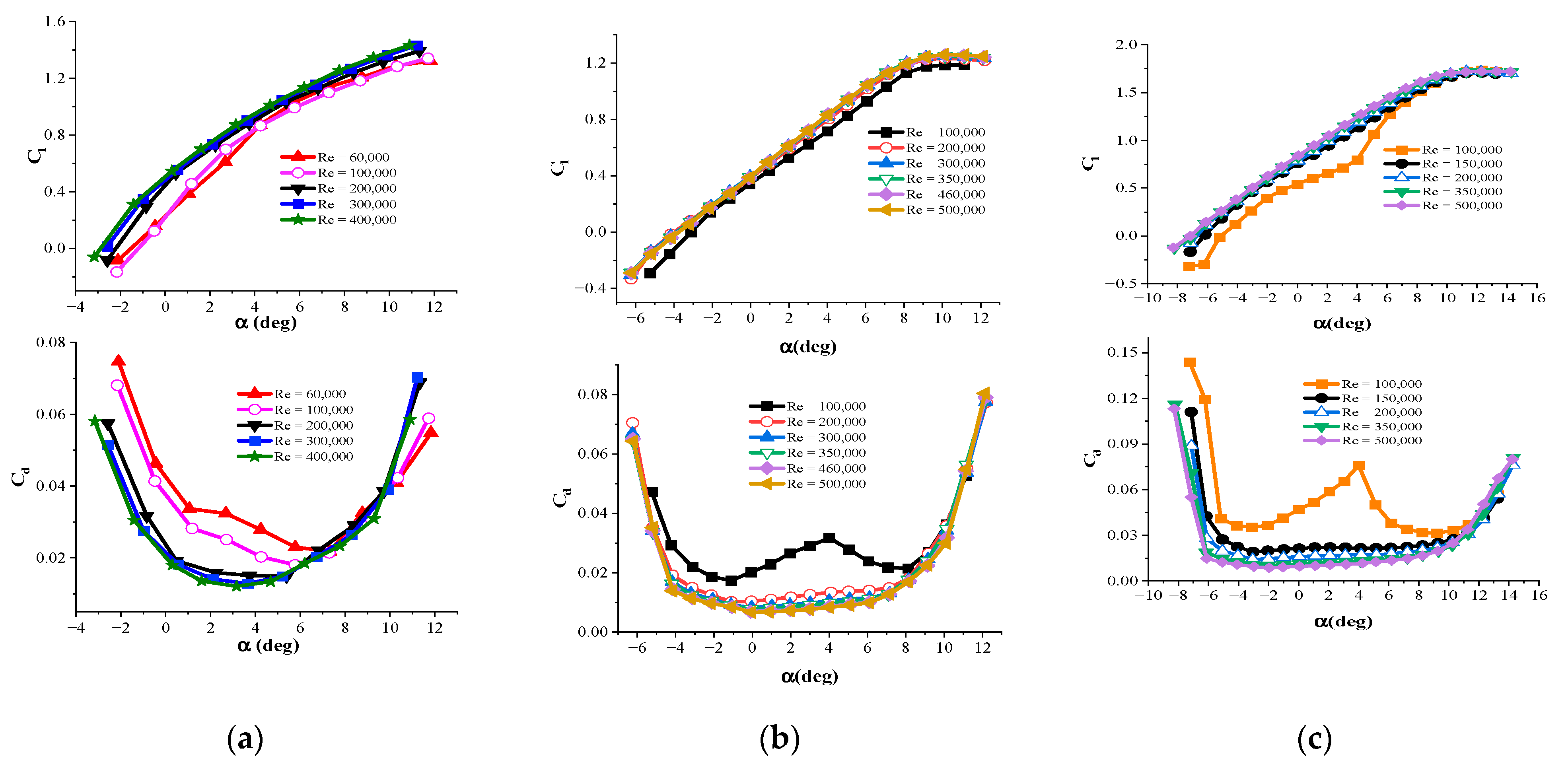
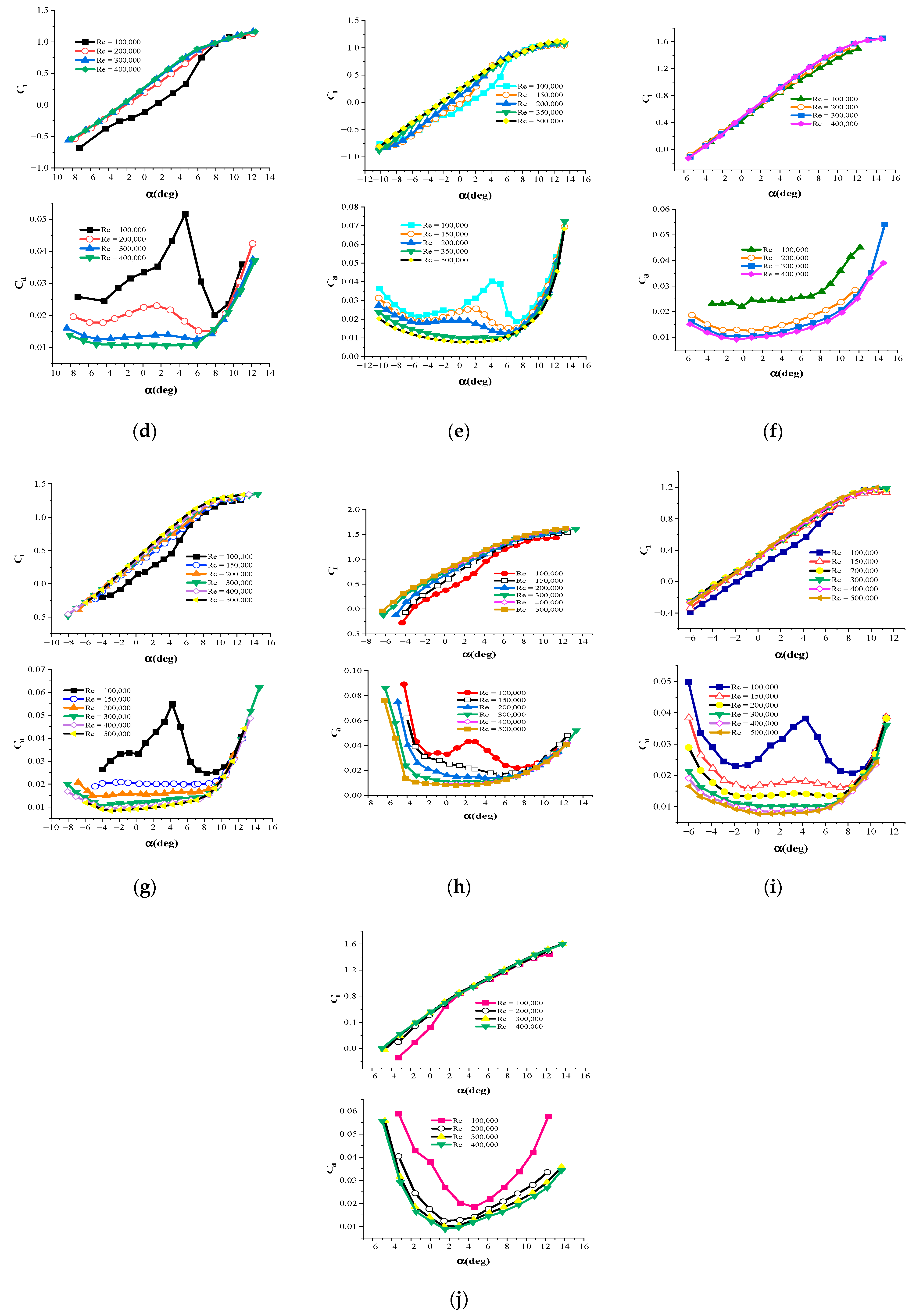
Despite the variety of airfoils available for use in large wind turbine blades, there are not many airfoils designed for SWTs. By examining previous research studies and also considering the operating Re of the turbine blade investigated in the present study, 10 airfoils that are used in the industry of SWTs, including, BW-3 [31], E387 [30], FX 63-137 [30], S822 [31], S834 [30], SD7062 [31], SG6040 [31], SG6043 [31], SG6051 [32], and USNPS4 [31] were selected for examination. Their aerodynamic coefficients, which are presented in Figure A1 of Appendix A, were tabulated and coded for various Re and angle of attack values, and they were employed in the numerical method. The geometry of the selected airfoils has been shown in Figure 1. In this figure, x/c indicates the distance along the chord line, while y/c shows the airfoil thickness normalized with the chord length.

3. Numerical Procedure

3.1. Multi-Objective Optimization

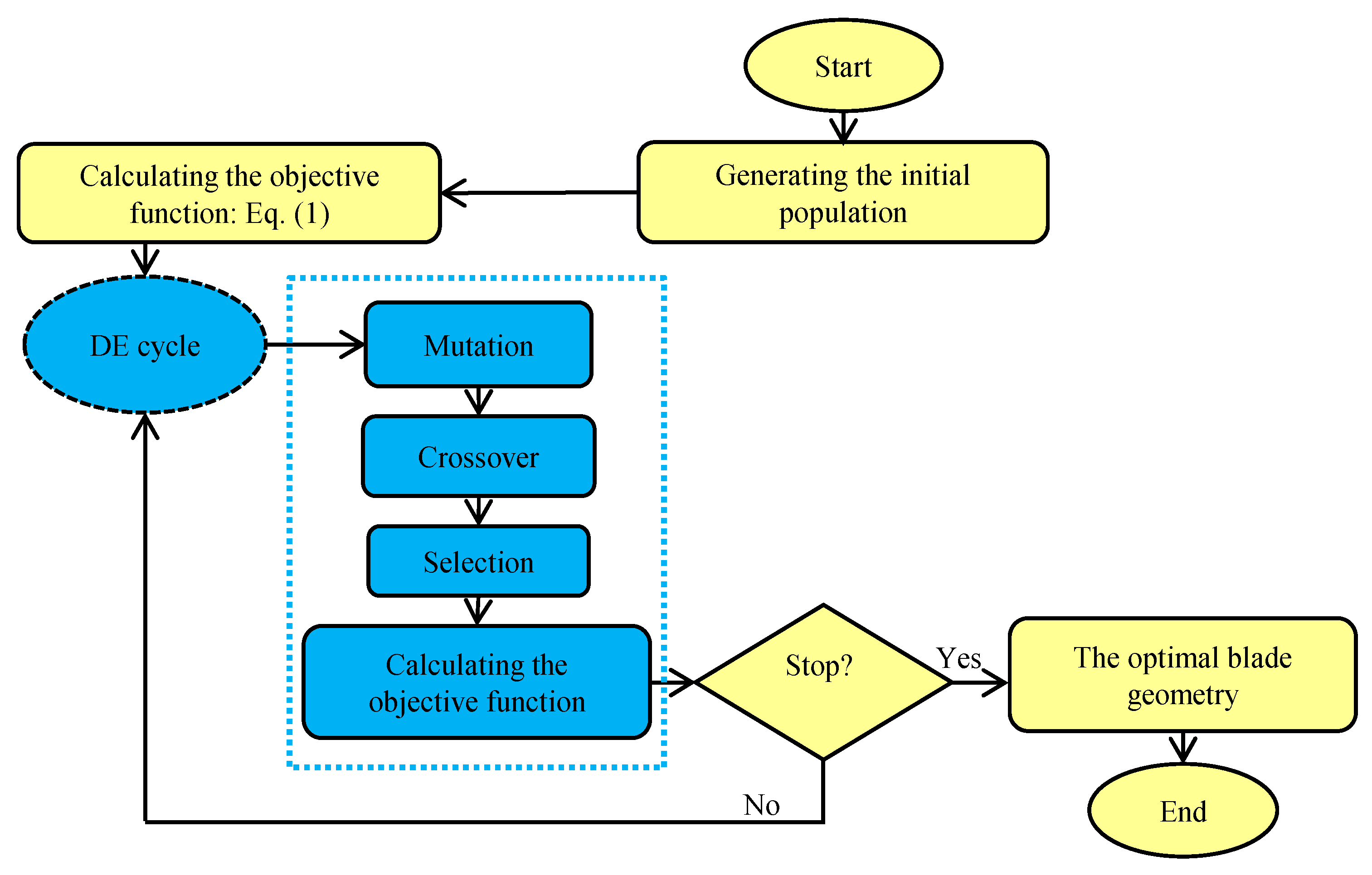
A multi-objective optimization was used to determine how to optimally distribute the twist angle and chord length along the blade for each of the selected airfoils to maximize the Cp and minimize Ts. For this purpose, in the present study, the differential evolution (DE) algorithm which was first introduced by Storn et al. [33] in 1997 was employed. DE is a population-based method that, among the recently presented metaheuristic search algorithms (MSAs), has become one of the most popular ones for solving optimization problems [34]. Presenting better global convergence and robustness, simpler and more straightforward implementation, as well as having good performance in solving multi-objective optimization problems, are the main factors that make this algorithm superior to other MSAs [35]. In this algorithm, the initial population (blades) is generated completely randomly, based on the upper and lower limits of the design variables. Then, using mutation and crossover operators, children (new blades) are generated. Subsequently, with the help of the selection operator, each child is compared with the parent which generated it. If the child has a better objective evaluation, it replaces the parent, and the next generation is generated. This process is repeated in the same way until the termination criteria are met. In the present study, the termination criterion was the number of generations. Although raising this number (500 generations in this study) increases the computation time, it guarantees to reach the global solution. It is worth mentioning that to ensure that the obtained answer is a global one, the values of the objective function were monitored. Since its values remained unchanged for 100 consecutive generations, it was made sure that the answer is global and the solution can be terminated. Employing the weighted coefficient method [36], to maximize Cp and minimize Ts, the following objective function was considered [20]:
M a x i m i z e : n C P max C P + 1 n min T s T s
using which, the objective function tries to simultaneously maximize the Cp (the first goal) and minimize the Ts (the second goal). The weighting factor, n (0 < n 1 ) determines the influence of these two goals on the objective function. Values of max C P and min T s represent the blades with the highest Cp and also the fastest Ts, respectively, which are updated in each generation. In other words, in each generation, the blades are compared and those with the best Cp and Ts values become candidates and form max C P and min T s for that generation. When the solution proceeds to the next generation, a new set of max C P and min T s are specified. It is noteworthy that these values remain constant after a sufficiently large number of generations. This way, it is made sure that the DE algorithm approaches the optimal solution.

3.2. Calculating Design Goals

To calculate the C p , the first objective of the design, the blade element momentum (BEM) technique was employed. This theory, which is the most widely used engineering model for simulating wind turbine blades and propellers [37], was proposed in 1935 by Glauret [38]. BEM is the combination of the blade element method and momentum theory in which the blade is divided into several independent elements, each element having a specific twist angle and chord length. Figure 2 shows the velocities on a blade element, where U is the wind velocity, and U T is the total velocity, which is obtained according to the value of the velocity at the blade section ( U 1 ) and also the angular velocity of the turbine ( ω ). The angles shown in this figure are the angle of attack ( α ), twist angle ( θ ), and flow angle ( ϕ ). Based on the figure, ϕ can be calculated from the following equation:
ϕ = t a n 1 1 a U 1 + a r ω
where a and a represent the axial and rotational induction factors, respectively, whose values are calculated in an iterative process [19].
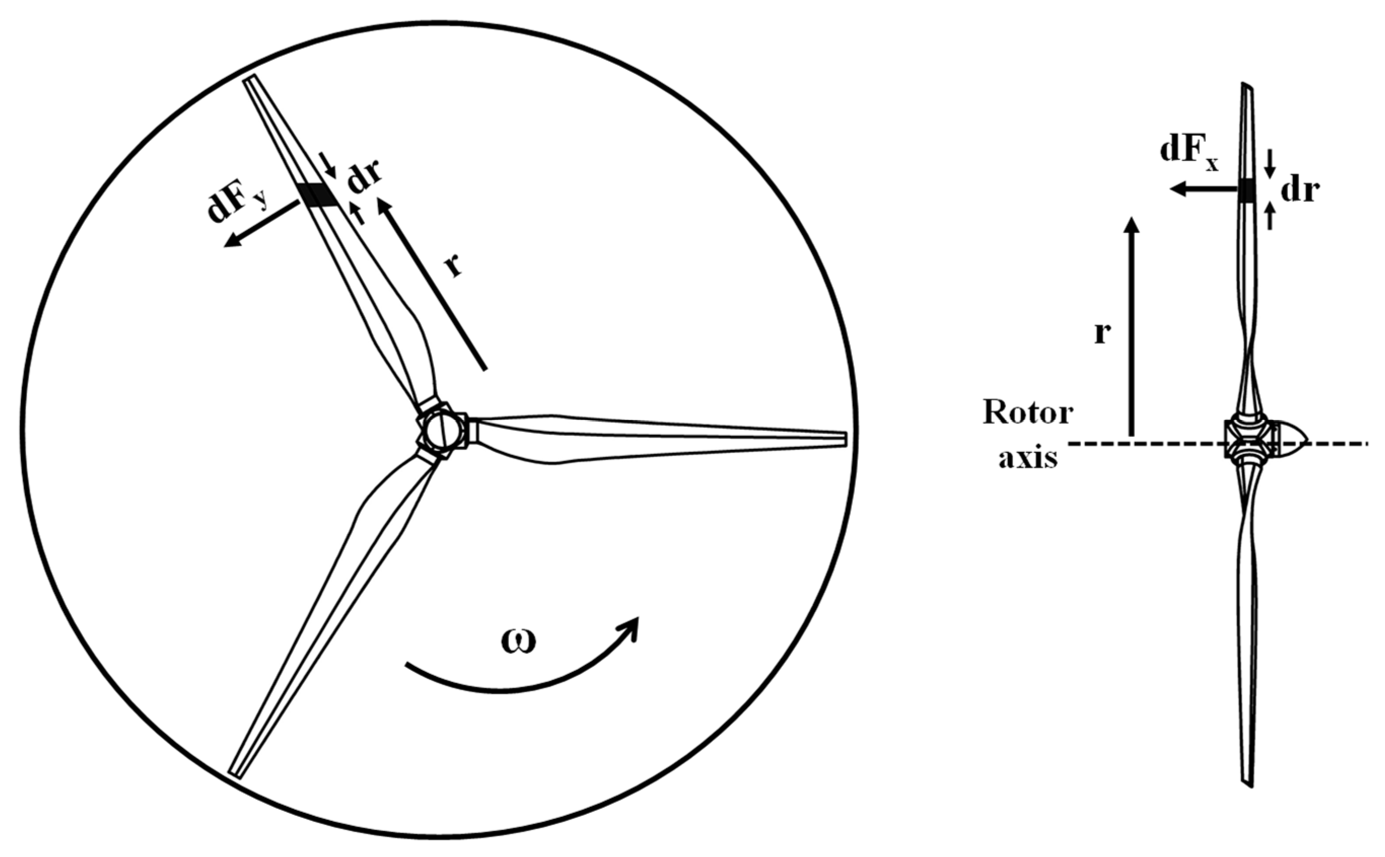
Figure 3 shows the axial ( d F x ) and tangential ( d F y ) forces on a blade element. Using the continuity equation along with the momentum equations for each element, the local values of axial force and aerodynamic torque d Q are calculated from:
d F x = 1 2 ρ U T 2 c d r   C l c o s ϕ + C d s i n ϕ
d Q = r   d F y = 1 2 ρ U T 2 c r d r   C l s i n ϕ C d c o s ϕ
In the above equations, ρ is the air density, r is the radial distance from the rotor hub, c is the chord length, and C l and C d are the lift and drag coefficients for the blade element, respectively. By summing the torque generated by each element, the total aerodynamic torque Q is calculated.
Finally, the C p of the turbine is calculated from [39]:
C p = Q ω 0.5 ρ S U 3
in which, S is the swept area of the blades.
To take the tip losses into account, Prandtl’s model ( F ) is employed. The purpose of this work is to determine the effect of blade tip losses along the blade. This parameter, which is a function of the number of blades ( N ), flow angle (ϕ), and also the radial coordinate along the blade ( r ), is defined as follows [40]:
F = 2 c o s 1 e f π
f = N R r 2 r s i n ϕ
By using the BEM theory and using analytical correlations for aerodynamic coefficients at high angles of attack, it is possible to determine the T s from the stationary state. Wood [41] showed that at high α values, from an aerodynamic viewpoint, airfoils behave like a two-dimensional flat plate, and to calculate their lift and drag coefficients, the following equations can be used with acceptable accuracy and regardless of the airfoil type:
C l = s i n 2 α
C d = 2   s i n 2 α
By implementing Equations (8) and (9) in Equation (4) and normalizing c and r with the blade tip radius ( R ), and also all speeds ( r ω , U T , and U 1 ) with the wind velocity ( U ) the startup torque Q S is calculated as follows:
Q S = N ρ U 2 R 3   r h 1 ( 1 + λ r 2 ) 1 / 2 c r   s i n θ   c o s θ λ r s i n θ d r
where, r h is the hub radius, and λ r = r ω / U represents the local tip speed ratio. From the assumption that no power is generated throughout the startup time and the aerodynamic torque is merely used to rotate the blades from the stationary state, the variation in the tip speed ratio can be computed using the following ordinary differential equation [20]:
d λ d t = R Q s Q r J U
in which, λ = R ω / U is the tip speed ratio, Q r shows the generator resistive torque, and J indicates the total rotational inertia, which is the sum of the blade inertia ( J b ) and the generator inertia ( J G ). By considering a specific value for the tip speed ratio (λ), this equation is solved and the time to reach λ from the stationary state ( λ = 0 ) to the specific value (which is considered in advance) is calculated. The value of λ = 1 is considered the ending point of the startup process and the above equation is solved using this method. It is necessary to explain that the parameters such as R , Q r , and also U , are constant values in the present study.
By normalizing c and r by R, the moment of inertia of the blade is determined from [19]:
J b = N ρ b A R 5 c r 2 d r + 1 12 c 4 c o s 2 θ d r + A 2 c 4 s i n 2 θ   d r
in which, ρ b is the density of the blade, and A is the surface area of the airfoil used in the blade, assuming that the unit is chord length.
It should be noted that the startup performance of a 5 kW wind turbine measured by Sessrego and Wood [42] has confirmed the accuracy of Equation (11). This reference indicates that the startup stage involves two important steps: (1) the long idling step, in which the blade has a slow rotational acceleration and continues until the angles of attack along the blade fall to less than 20°, and (2) the rapid acceleration step, in which the blade reaches an operational angular velocity. Therefore, to minimize the startup time, the initial phase should be minimized. Integrating Equation (11) up to λ = 1 properly captures this step. To calculate Equation (11), the Adams–Moulton method was used and the trapezoidal integration method was employed to calculate the blade inertia of Equation (12).

3.3. Adjusting the Input Parameters

The flowchart of the used optimization algorithm is illustrated in Figure 4. A code that was developed in MATLAB software was employed for the optimization process and calculation of the design objectives.
Based on the values suggested in the literature [19,43], the blade was divided into 15 elements. Table 1 shows the minimum and maximum values of the design variables according to the limitations and construction problems for the twist angle/chord length distribution. Additionally, Table 2 lists the input parameters considered in the DE algorithm.
The selected small horizontal-axis wind turbine was introduced and numerically evaluated by Pourrajabian et al. [44]. The technical specifications of this turbine, which include the output power (P), number of blades (N), blade radius (R), hub radius ( r h ), angular velocity ( ω ), rated tip speed ratio ( λ r a t e d ), rated wind speed ( U r a t e d ), generator inertia ( J G ), generator resistive torque ( Q r ), blade density ( ρ b ), startup wind speed ( U s ), and the type of airfoil used in the blade are given in Table 3.

3.4. Validation of the BEM Code

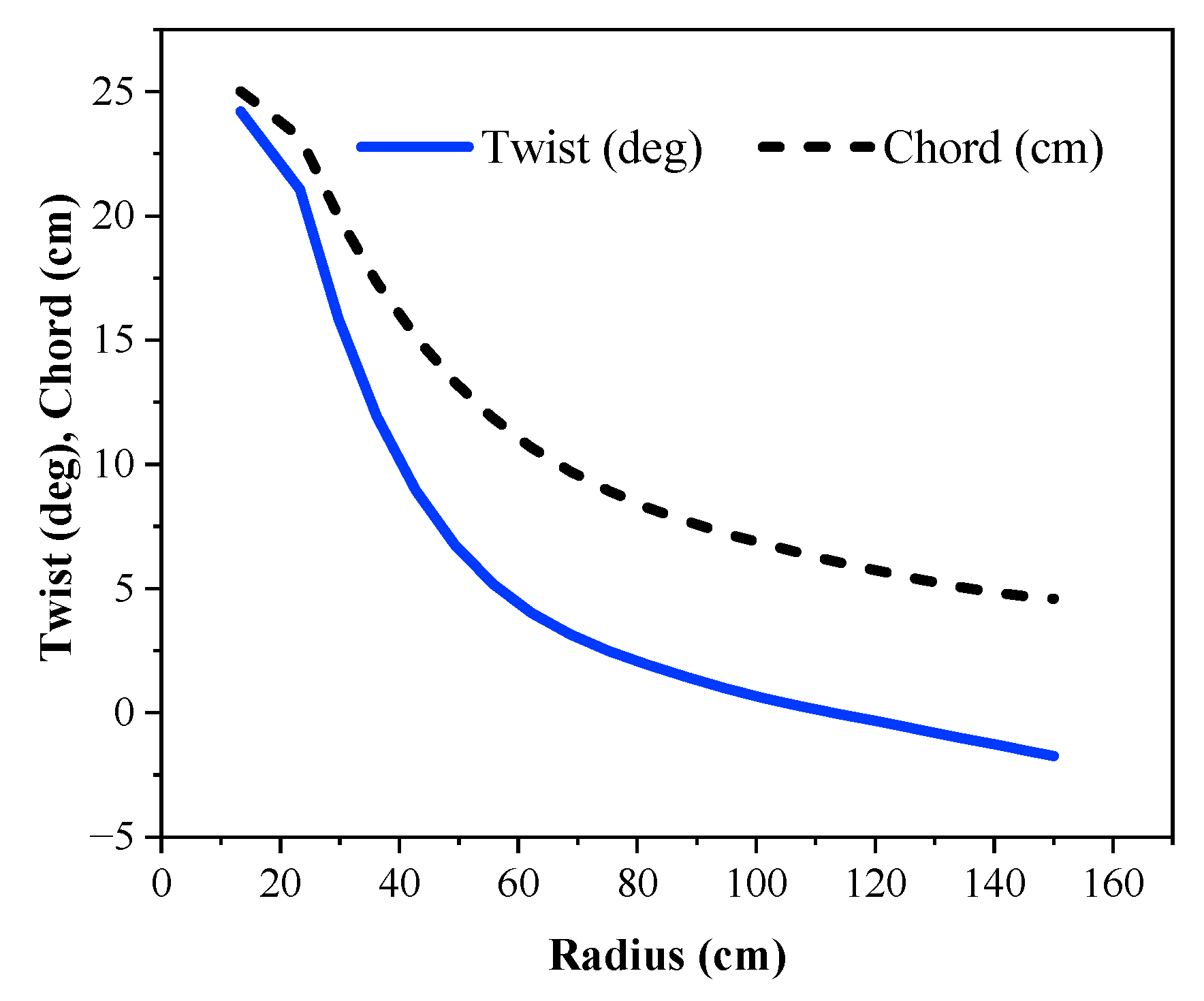
To evaluate the accuracy of the developed BEM code, the results of the present study have been validated with the experimental results from the wind tunnel test of a small wind turbine with a radius of 1.5 m. This two-bladed turbine was examined by Anderson et al. [45], and then further investigated by Wood [19] and Spera [37]. The geometry of this turbine, which uses NACA4412 airfoil as the blade cross-section, is shown in Figure 5.
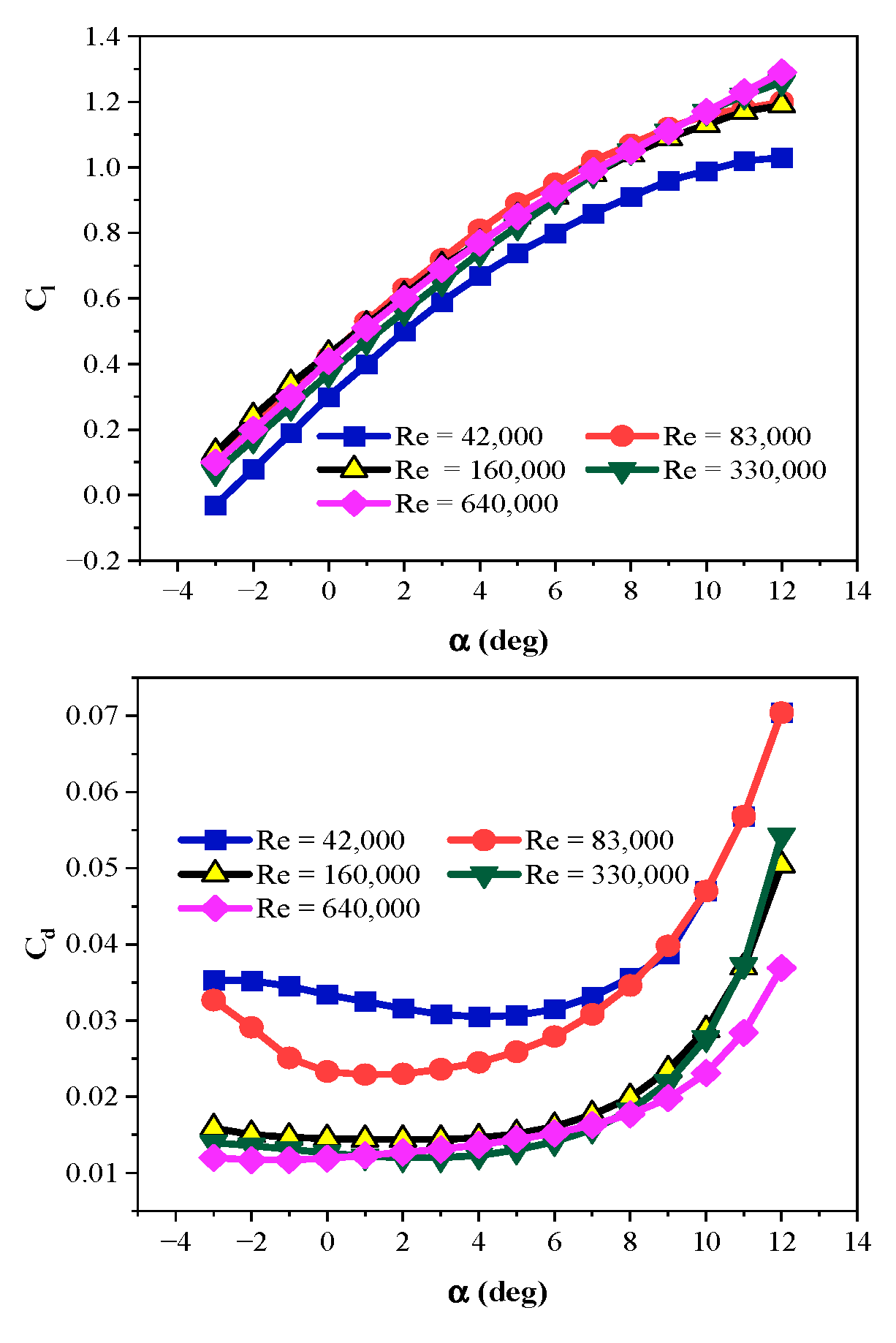
The aerodynamic coefficients of the NACA4412 airfoil, including the lift and drag coefficients at various angles of attack and different Reynolds numbers, are also depicted in Figure 6.
As mentioned in Section 2, all aerodynamic coefficients of the airfoils used in the present study are coded, and, based on the Re number and the angle of attack of each blade element, the corresponding values of Cl and Cd are computed and called during the BEM calculations and optimization steps.
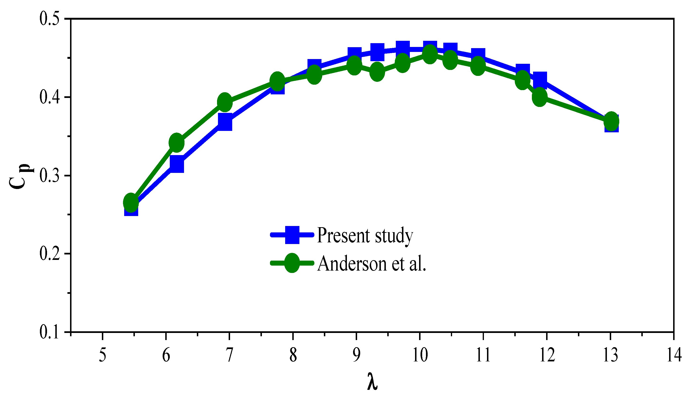
Figure 7 shows the changes of Cp at different λ values. It can be observed that the results obtained from the developed numerical code are well-compatible with the experimental results with a maximum error of 6.47%. It is noteworthy that the mean squared error (MSE) of the obtained numerical values was found to be 0.000228562. More detailed data for this comparison are given in Table A1 in Appendix B.

3.5. Validation of the Optimization Code

The ideal equations proposed by Burton et al. [46] were employed to evaluate the performance of the optimization code. By ignoring the tip losses and drag, the following correlations determine the twist angle and the chord length along the blade to achieve the maximum power coefficient:
tan ϕ = 2 3 λ r + 2 λ r
c C l = 16 π 9 N λ 4 9 + λ r + 2 9 λ r 2
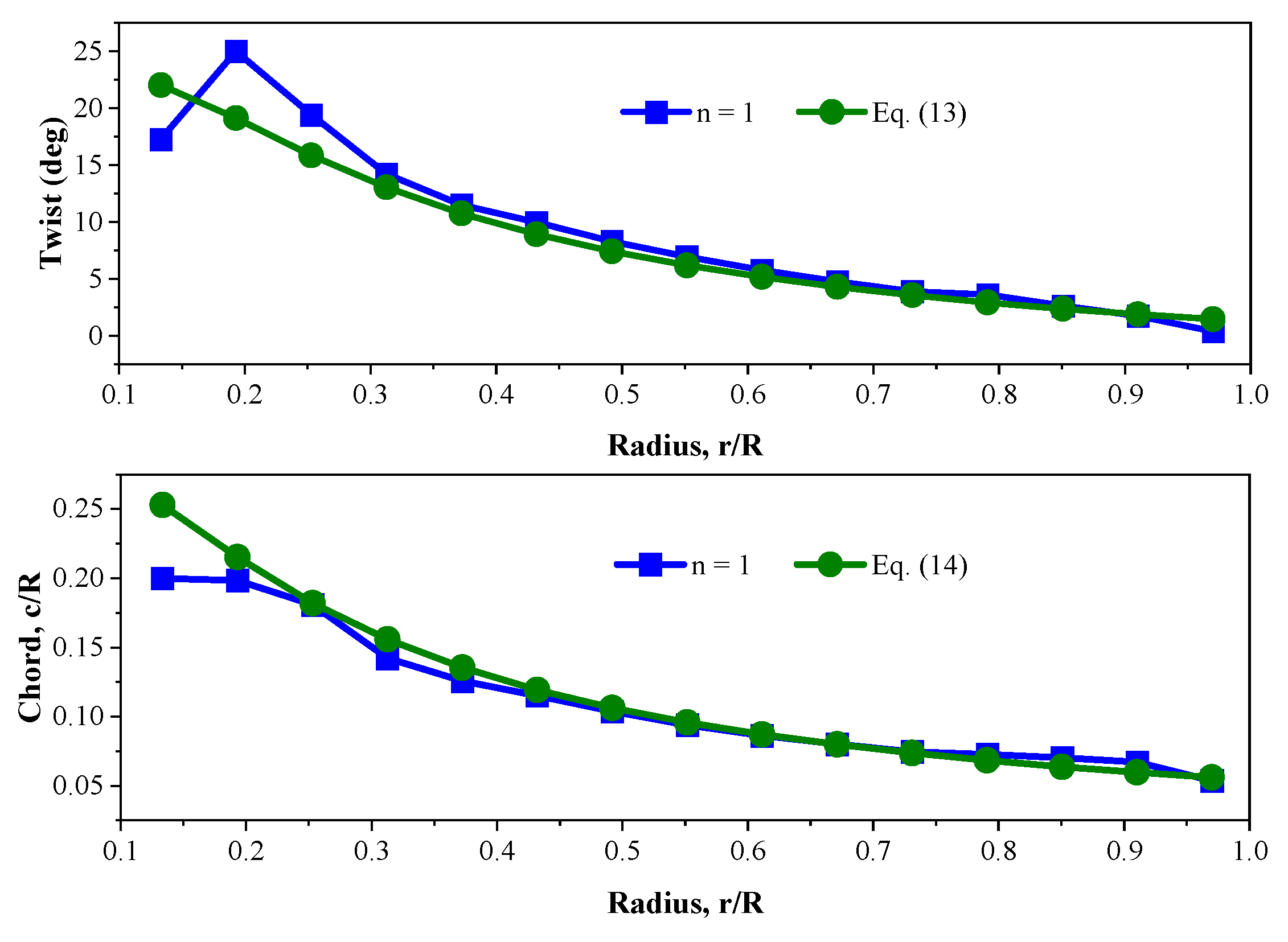
Considering the BW-3 airfoil for the 1 kW turbine blade of the present study, Figure 8 shows the distribution of the twist angle (θ) and chord length (c) obtained from the optimization algorithm (n = 1) and the ideal Equations of (13) and (14).
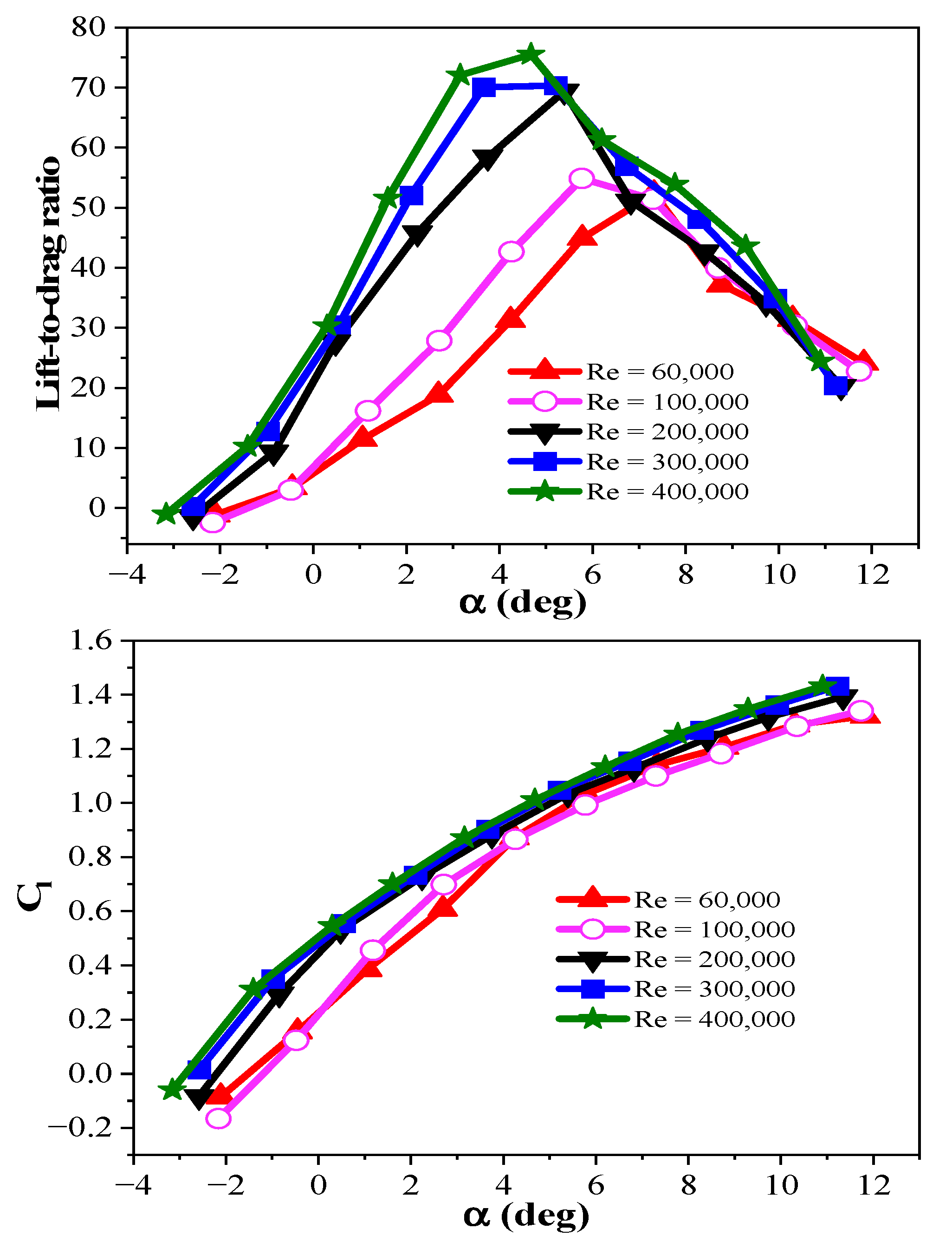
As can be observed, there is a good agreement between the distributions along the blade. Therefore, it is ensured that the final answer of the optimization code is optimal. Of course, there are some discrepancies in the distributions considered by the optimization algorithm in the root section, the reason for which is revealed in detail in the next section. It should be noted that, to use the ideal Equations (13) and (14), it is necessary to specify the α and Cl values of the airfoil at the maximum lift-to-drag ratio, which, according to Figure 9, are 5.39° and 1.034, respectively, for the BW-3 airfoil at the Re of 200,000.

4. Discussion of Results

Similar to the specified ranges for the design variables (mentioned in Table 1) and also the value of Table 2 and Table 3, n is an input parameter for running the optimization. In multi-objective optimization problems, there is no single answer. In this study, the answers are determined by changing the value of n in the objective function (Equation (1)), which leads to the Pareto front. Here, Pareto front members are the blades whose at least one component of the objective function has a larger Cp or 1/Ts value than the other blades. Generally, larger values are considered for n, because the output power is a more important goal than the startup time [19]. Imposing low weighting factors (n) causes poor aerodynamic performance of the blade and makes it practically unusable. Selecting the final blade from the Pareto front depends on the wind potential. Although n = 1 is used in windy areas to achieve the maximum power coefficient, n = 0.8 is recommended in areas with low wind speeds where the startup performance of turbines is more important [20,21].
By considering the input parameters mentioned in Section 3.3, as well as the explanations provided above, the optimization process was used to evaluate the performance of the selected airfoils, the results, which include Cp and Ts, are summarized in Table 4. It is necessary to explain that the details of the optimization results were also obtained for n = 0.6, and the tabulated results can be found and compared in Table A2 of Appendix C.

4.1. Investigating the Performance of Airfoils in Windy Areas

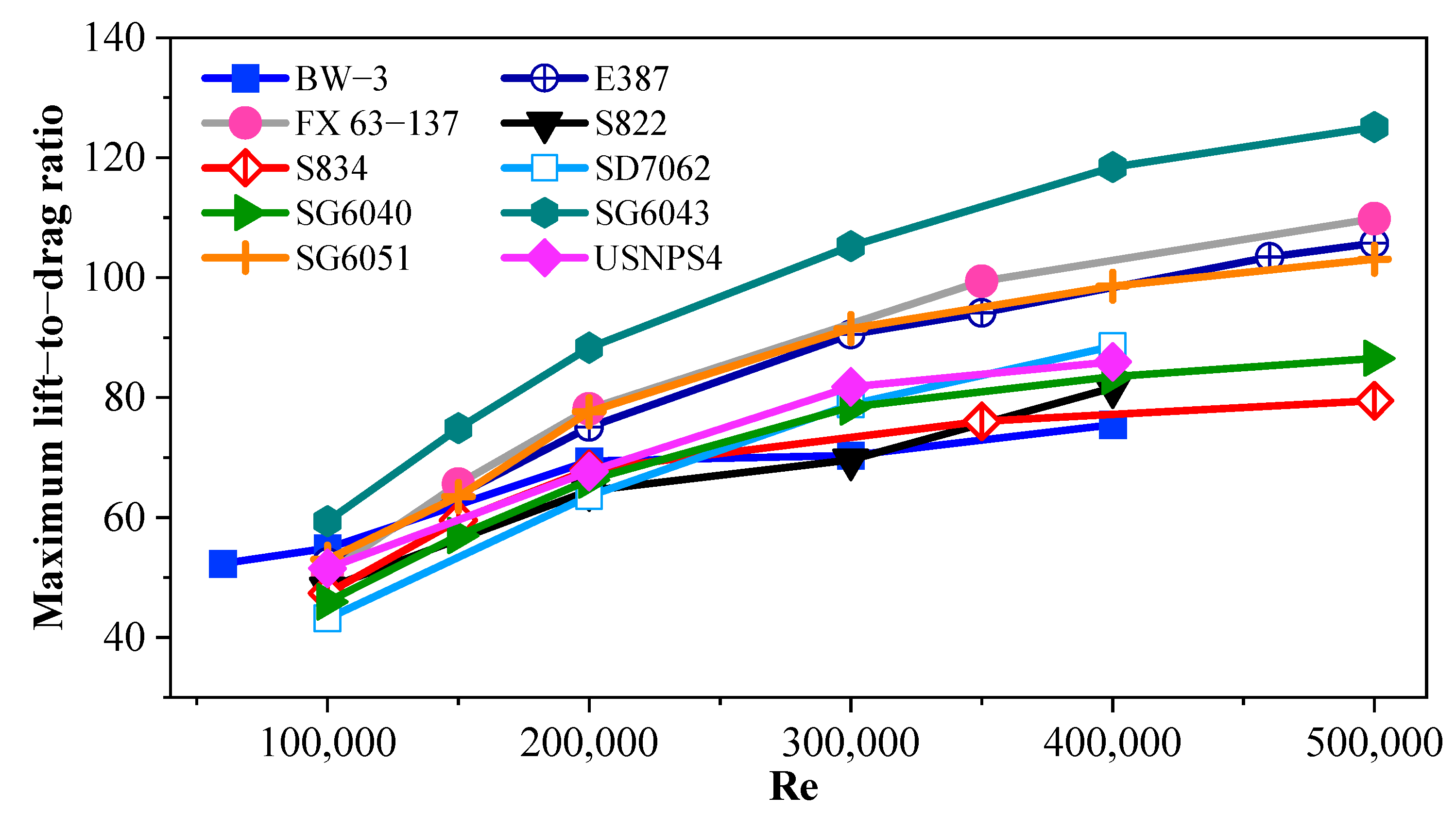
In areas with high wind speeds (n = 1) where Ts is removed from the objective function, the SG6043 airfoil yields the highest Cp while the S822 and SG6040 airfoils present the lowest Cp (see Table 4). The lift-to-drag ratio of airfoils is an important parameter in the efficiency of wind turbine blades. Figure 10 shows the maximum lift-to-drag ratio of the selected airfoils over a wide range of Re numbers.
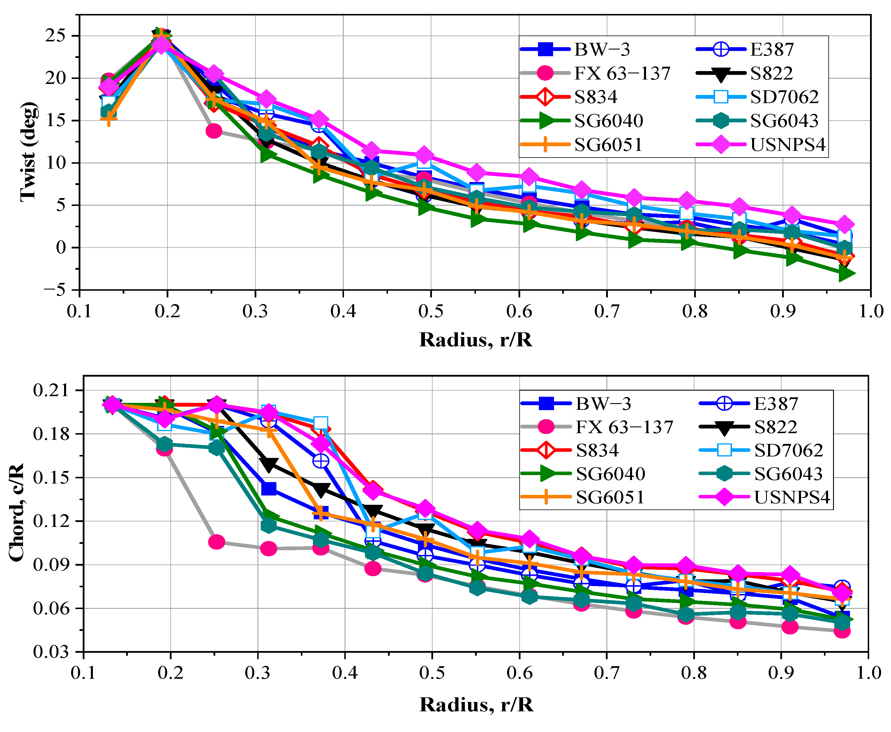
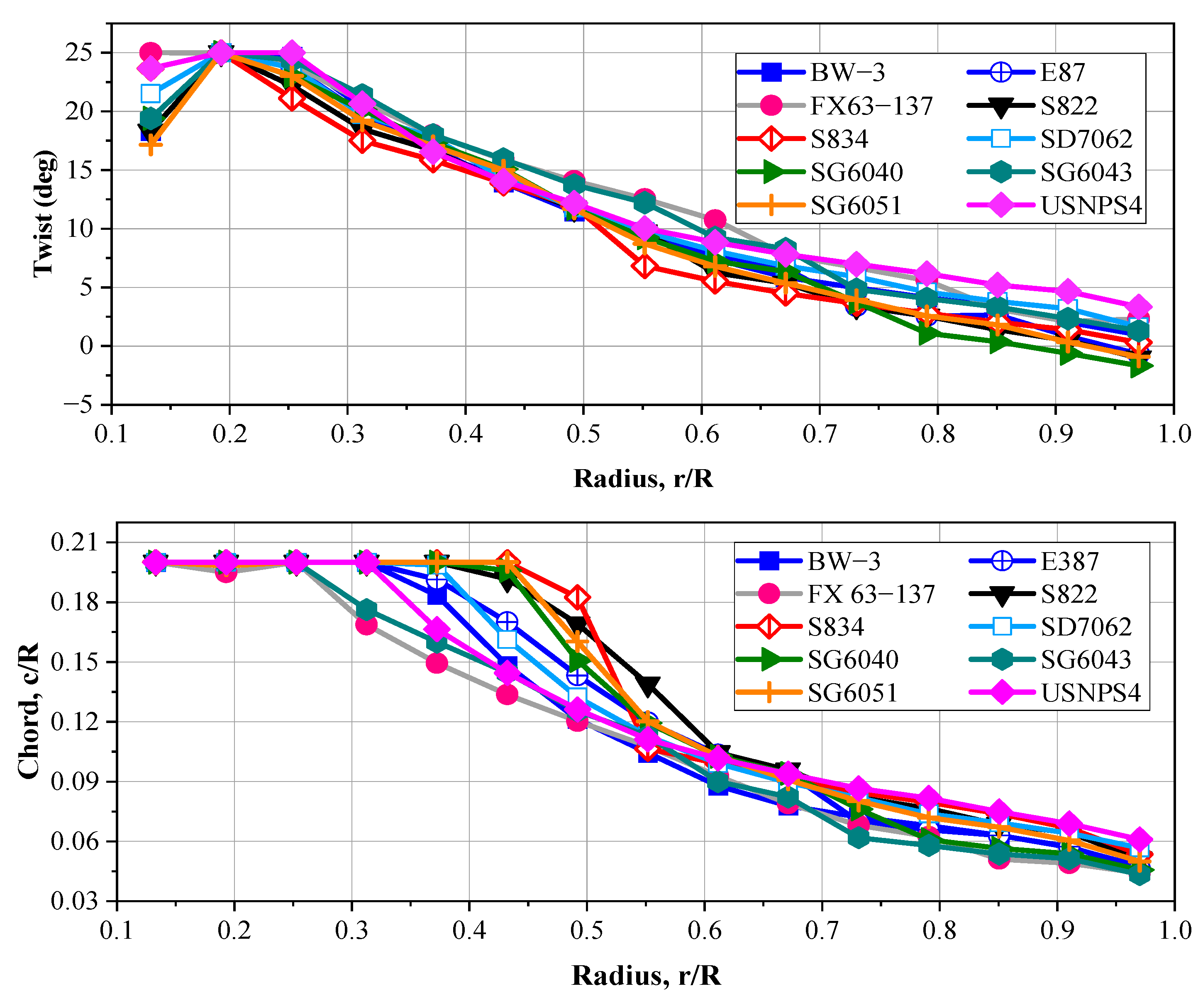
It can be observed that, compared to the other airfoils, this value is higher for the SG6043 airfoil. It should be noted that the type of airfoil completely influences the distribution of twist and chord along the blade. Indeed, the optimization algorithm considers the best geometry for the blade based on the aerodynamic coefficients and geometric characteristics of each airfoil. Figure 11 shows the distribution of twist and chord of the selected airfoils for n = 1.
By focusing on this figure, it can be seen that the values of the chord length for the blade that was fitted with the FX 63-137 airfoil are smaller than the values considered for the other selected airfoils. Due to this, despite the high lift-to-drag ratio of this airfoil (Figure 10), the Cp is not so high. Because the smaller chord length leads to a lower Re and, hence, reduces the lift-to-drag ratio. The opposite is true for the USNPS4 airfoil. According to Figure 10, it can be observed that this airfoil does not have a high lift-to-drag ratio, but the larger chord length values of the blade fitted with this airfoil increase the Re and, consequently, raise the Cp.
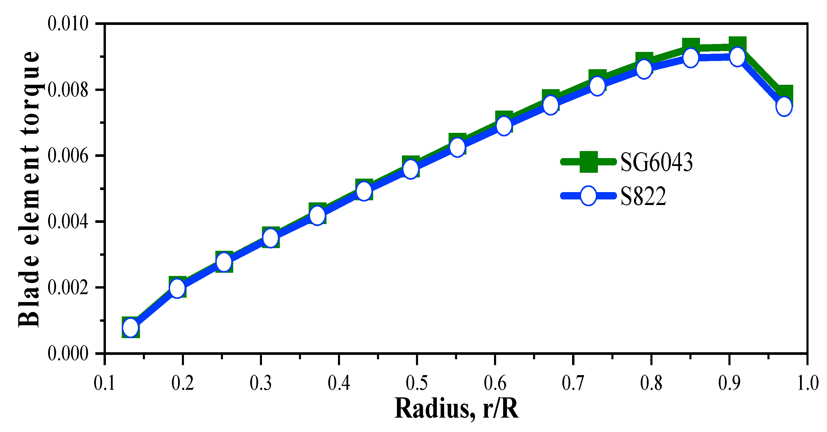
It should be noted that for all selected airfoils, the twist angles and chord lengths are not smooth at the root elements (as seen in Figure 8). This is due to the low contribution of these elements in the total aerodynamic torque and, hence, the Cp of the turbine, which makes the optimization algorithm focus on the evolution of the design variables in the middle and tip elements and creates a smoother distribution in these elements. To take a closer look at this point, Figure 12 illustrates the torque generation distribution along the blade throughout the power generation for the SG6043 and S822 airfoils.
As can be seen, regardless of the airfoil type, a significant portion of the aerodynamic torque is generated by the middle and tip elements of the blade, and the share of the root elements is considerably smaller. It should be noted that the slight decrease in the aerodynamic torque at the tip of the blade is because of considering the blade tip losses in the BEM calculations.

4.2. Investigating the Performance of Airfoils in Areas with Low Wind Speed

In areas with low wind speeds (n = 0.8), small wind turbines need to react quickly to the wind and start generating power in the shortest possible time. In this regard, Worasinchai et al. [18] have shown that reducing startup time increases energy capture.
According to Table 4, the startup performance of the BW-3 airfoil is better than the other selected airfoils. Thus, the turbine that uses this airfoil has the shortest Ts. The reason is the low inertia of the blades fitted with this airfoil (see Figure 13).
The S822, S834, and SG6040 airfoils have the highest Ts and their application in areas with low wind speeds is not recommended at all. The common aspect of these three airfoils is their high surface area compared to the other selected airfoils, which is an effective factor in the blade moment of inertia, aside from the chord length (Figure 14).
But it is also important to note that a thinner airfoil does not always present a better performance at low wind speeds. For example, the E387 airfoil is thinner than the SG6043 airfoil and has a smaller surface area (see Figure 14), but it has a longer Ts (Table 4 for n = 0.8). The reason is the higher moment of inertia and the lower startup torque (the startup torque is examined at the end of the current section) of the blades fitted with this airfoil compared to the blades fitted with the SG6043 airfoil.
Figure 15 shows the optimal distribution of twist and chord for the selected airfoils for n = 0.8. By comparing this figure with Figure 11, it can be observed that regardless of the airfoil type, raising the twist and chord values in the root part of the blade decreases the Ts. It should be noted that during the startup process, the angles of attack along the blade are high, which decrease by raising the twist angle, and this increases the startup torque. However, since the blade root elements have a smaller share in power generation, the optimization algorithm applies these increments (twist and chord) only in this area so that the Cp does not decline much.
Figure 16 shows the variations of startup torque during the startup time of the selected airfoils for n = 0.8. Regardless of the airfoil type, as the blade begins to rotate, the startup torque initially decreases, and then it starts to increase. When the blade is stationary, the drag force is perpendicular to the direction of rotation and does not affect the startup torque. As the blade begins to rotate, the drag force reduces the startup torque, but then the startup torque starts to increase.
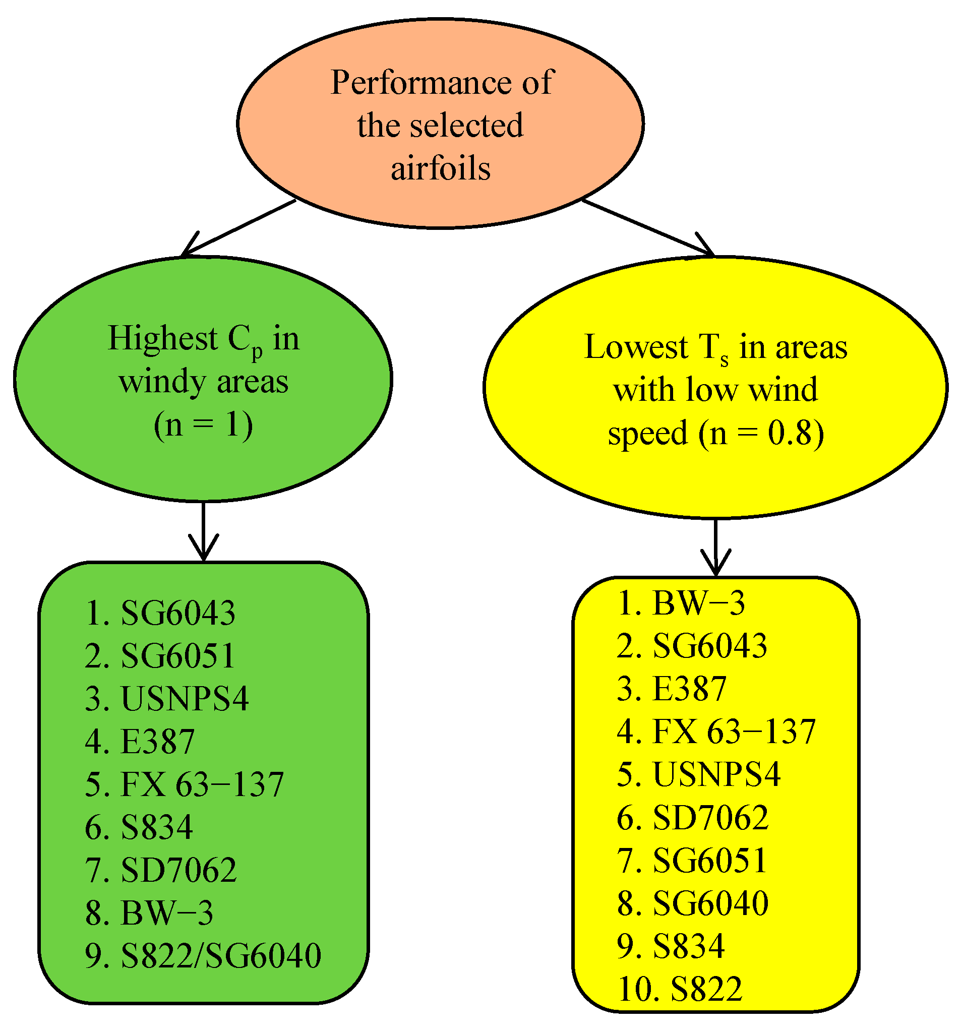
Figure 16 shows that the blade that uses the USNPS4 airfoil produces the highest startup torque, but having a high moment of inertia raises its Ts. The lowest startup torque is produced in the blade with the BW-3 airfoil, but, as mentioned, its low moment of inertia is the advantageous aspect of this airfoil in areas with low wind speed. It is noteworthy that the startup torque is a function of two parameters, including the twist angle and the chord length (see Equation (10)). The difference observed in the values of startup torque for the selected airfoils is due to the different twist angle and chord length values that the optimization algorithm has considered for each airfoil. Finally, Figure 17 summarizes the performance of the selected airfoils in terms of Cp and Ts. The arrangement of these airfoils is based on exhibiting the highest Cp in windy areas and having the shortest Ts in areas with low wind speeds.

5. Conclusions

In the present study, the effect of the airfoil type was investigated on the power coefficient, as well as the startup time of a 1 kW small wind turbine by developing a numerical code. For this purpose, 10 airfoils, namely, BW-3, E387, FX 63-137, S822, S834, SD7062, SG6040, SG6043, SG6051, and USNPS4, were selected and the differential evolution (DE) optimization technique was employed to determine the best geometric shape of the blades. The twist angle and chord length were considered as design variables while maximizing the power coefficient and minimizing the startup time were defined as design goals. The blade element moment (BEM) method was used to calculate the power coefficient and the startup time. The BEM code and the optimization tools were both validated. The main results can be summarized as:
  • Regardless of the type of airfoil, using ideal equations to determine the twist angle and chord length to maximize the power coefficient, raises the turbine startup time;
  • The SG6043 airfoil has the highest power coefficient while the S822 and SG6040 airfoils have the lowest power coefficients. The reason for the superiority of SG6043 is its high lift-to-drag ratio. It is highly recommended to use this airfoil in windy areas where the purpose of designing small wind turbines is to achieve the maximum power coefficient;
  • Among the optimal blades for achieving the maximum power coefficient, the blades with the FX 63-137 and USNPS4 airfoils have the shortest and longest chord lengths, respectively. This has caused the power coefficient not to be as high as expected, despite the high lift-to-drag ratio of the FX 63-137 airfoil;
  • Regardless of the airfoil type, raising the twist angle and chord length in the root section reduces the turbine startup time;
  • From the startup viewpoint, the BW-3 airfoil has the best performance among the selected airfoils. This is due to the low inertia of the blades fitted with this airfoil. Therefore, in areas with low wind speeds where having a low startup time is greatly important, the use of this airfoil is highly recommended;
  • The S822, S834, and SG6040 airfoils have the highest startup time. The common aspect of these three airfoils is their high surface area;
  • Although the thinness of the airfoil is an advantage for reducing the blade moment of inertia and hence obtaining a better performance of the turbine at low wind speeds, the blade fitted with a thinner airfoil does not necessarily have a lower startup time than the blade with a thicker airfoil. This is because the airfoil type completely affects the distribution of twist angle and chord length. This is accompanied by fundamental changes in the startup torque and moment of inertia, both of which play an influential role in the startup process of the turbine;
  • Regardless of the airfoil type, when the blade begins to rotate, the startup torque first decreases slightly and then starts to increase;
  • The highest startup torque is produced by the blade fitted with the USNPS4 airfoil and the lowest startup torque is produced by the blade fitted with the BW-3 airfoil.

Author Contributions

Conceptualization, V.A.; methodology, V.A., M.N. and R.K.; software, V.A.; validation, V.A.; formal analysis, R.K.; investigation, V.A.; resources, F.A.; data curation, V.A.; writing—original draft preparation, V.A. and F.A.; writing—review and editing, F.A. and W.Y.; visualization, F.A.; supervision, M.N., R.K. and W.Y.; project administration, M.N.; funding acquisition, W.Y. All authors have read and agreed to the published version of the manuscript.

Funding

This research received no external funding.

Institutional Review Board Statement

Not applicable.

Informed Consent Statement

Not applicable.

Data Availability Statement

The data presented in this study are available on reasonable request from the corresponding author.

Conflicts of Interest

The authors declare no conflict of interest.

Nomenclature

A Airfoil cross-sectional area [m2]
a Axial induction factor
a Rotational induction factor
C d Drag coefficient
C l Lift coefficient
C P Power coefficient
c Blade chord [m]
F Prandtl tip loss factor
F x Axial force [kg·m·s−2]
F y Total tangential force [kg·m·s−2]
f Term in Prandtl tip loss factor
J Rotational inertia [kg·m2]
N Number of blades
n Weighting factor
P Power [kg·ms−3]
Q Torque [kg·m2·s−2]
Q r Resistive torque [kg·m2·s−2]
Q s Startup torque [kg·m2·s−2]
Q s 0 Startup torque at t = 0 [kg·m2·s−2]
R Blade tip radius [m]
R e Reynolds number
r Radial coordinate along blade [m]
t Time [s]
S The swept area of the blades [m2]
T s Startup time [s]
U Wind velocity [m·s−1]
U r a t e d Wind velocity for rated power [m·s−1]
U T Total velocity at blade element [m·s−1]
Greek Symbols
α Angle of attack
θ Blade twist angle
λ Tip speed ratio
λ r a t e d Tip speed ratio for rated power
λ r Local tip speed ratio
ρ Density [kg·m−3]
ϕ Blade inflow angle
ω Angular velocity [s−1]
Subscripts
1The upwind face of the rotor
bBlade
GGenerator
hHub
sStartup
Abbreviations
BEMBlade element momentum
DEDifferential evolution algorithm
HAWTHorizontal-axis wind turbine
NACAU.S. National Advisory Committee on Aeronautics

Appendix A

Figure A1 illustrates the changes in Cl and Cd values for different airfoil blades which were investigated throughout this research. These values were fed into the developed numerical code as a database for the current numerical computations. It is necessary to explain that, in addition to the relevant references, these coefficients are also available on the website maintained by Professor Michael Selig’s group at the University of Illinois at www.ae.illinoise.edu/m-seliq/ (accessed on 5 August 2022). Numerous researchers in this field have employed the data acquired from this website for their study [48,49,50,51], and the use of this website as a valid source for obtaining lift and drag coefficient values was recommended in a reference book [19].
Figure A1. Changes of the Cl and Cd values for (a) BW-3 [31], (b) E387 [30], (c) FX 63-137 [30], (d) S822 [31], (e) S834 [30], (f) SD7062 [31], (g) SG6040 [31], (h) SG6043 [31], (i) SG6051 [31], and (j) USNPS4 [31].
Machines 10 00687 g0a1aMachines 10 00687 g0a1b

Appendix B

Table A1 presents the Cp values from the current study and the experimental research of Anderson et al. [45]. This table also presents the deviation between these two sets of results.
Table A1. Detailed changes of Cp at different λ values for the current research and the study of Anderson et al. [45].
λCp
Current Numerical CodeExperimental Data [45]Absolute ErrorSquared ErrorError (%)
5.450.259600.264980.005382.89444 × 10−5 2.03
6.170.319630.341770.022140.000490186.47
6.930.368430.393250.024820.0006160326.31
7.7590.415060.419830.004772.27529 × 10−51.13
8.340.437150.42827−0.008887.88544 × 10−5−2.07
8.970.452410.44008−0.012330.000152029−2.80
9.3290.457680.43207−0.025610.000655872−5.92
9.730.460760.44346−0.01730.00029929−3.90
10.160.460810.45443−0.006384.07044 × 10−5−1.40
10.480.458290.44726−0.011030.000121661−2.46
10.9180.451140.43966−0.011480.00013179−2.61
11.620.431380.42152−0.009869.72196 × 10−5−2.33
11.890.421460.40000−0.021460.000460532−5.36
13.020.366780.368780.0024 × 10−60.54

Appendix C

Table A2 shows the optimal values of Cp, Ts, Jb, and QS0 for n = 1, 0.8, and 0.6 weighting factors. The values of n = 1 and n = 0.8 are two accepted values in the literature for the design of small wind turbine blades to operate in windy areas and areas with low wind speed, respectively. In this regard, the work of Pourrajabian et al. [20] and Rahgozar et al. [21] can be referred to. Considering small values for n results in impractical blades whose aerodynamic performance is poor. The table below summarizes the optimization results of the current research with n = 0.6, along with n = 1 and n = 0.8. As can be noticed from the table, regardless of the airfoil type, considering n = 0.6 drastically reduces the power coefficient, which is indeed the main goal of wind turbine blade design.
Table A2. The optimal values of Cp, Ts, Jb, and QS0 for selected airfoils for n = 1, 0.8, and 0.6.
AirfoilA
(m2)
n = 1n = 0.8n = 0.6
CpTs (s)Jb (kgm2)QS0 (Nm)CpTs (s)Jb (kgm2)QS0 (Nm)CpTs (s)Jb (kgm2)QS0 (Nm)
BW-30.03640.4962.780.4381.1650.4861.820.4941.6510.4351.330.3641.673
E3870.05730.5024.870.7861.2130.4853.100.8891.7220.4392.270.6601.753
FX 63-1370.08310.4998.440.5840.7950.4893.260.9641.7570.4492.590.7601.749
S8220.10870.49513.251.6001.0060.4817.022.0001.7110.4164.711.3371.725
S8340.10420.49811.541.8721.1930.4836.871.9211.6820.4114.371.1371.641
SD70620.08830.4976.151.3941.4350.4884.491.4211.8340.4383.311.0031.794
SG60400.10420.49515.671.1050.8170.4806.021.6781.6950.4294.311.2331.726
SG6043 0.06850.5065.720.5800.9720.4962.890.8421.7430.4592.330.6871.759
SG60510.08390.5049.801.2531.1180.4905.131.4561.7080.4283.450.9501.689
USNPS40.08840.5035.361.5861.7310.4934.221.4231.9190.4433.140.9871.836

References

  1. Afsharpanah, F.; Pakzad, K.; Mousavi Ajarostaghi, S.S.; Poncet, S.; Sedighi, K. Accelerating the Charging Process in a Shell and Dual Coil Ice Storage Unit Equipped with Connecting Plates. Int. J. Energy Res. 2022, 46, 7460–7478. [Google Scholar] [CrossRef]
  2. Shyu, C.-W. A Framework for ‘Right to Energy’ to Meet UN SDG7: Policy Implications to Meet Basic Human Energy Needs, Eradicate Energy Poverty, Enhance Energy Justice, and Uphold Energy Democracy. Energy Res. Soc. Sci. 2021, 79, 102199. [Google Scholar] [CrossRef]
  3. Karthikeyan, N.; Kalidasa Murugavel, K.; Arun Kumar, S.; Rajakumar, S. Review of Aerodynamic Developments on Small Horizontal Axis Wind Turbine Blade. Renew. Sustain. Energy Rev. 2015, 42, 801–822. [Google Scholar] [CrossRef]
  4. Afsharpanah, F.; Mousavi Ajarostaghi, S.S.; Arıcı, M. Parametric Study of Phase Change Time Reduction in a Shell-and-Tube Ice Storage System with Anchor-Type Fin Design. Int. Commun. Heat Mass Transf. 2022, 137, 106281. [Google Scholar] [CrossRef]
  5. Afsharpanah, F.; Cheraghian, G.; Hamedani, F.A.; Shokri, E.; Ajarostaghi, S.S.M. Utilization of Carbon-Based Nanomaterials and Plate-Fin Networks in a Cold PCM Container with Application in Air Conditioning of Buildings. Nanomaterials 2022, 12, 1927. [Google Scholar] [CrossRef] [PubMed]
  6. Afsharpanah, F.; Pakzad, K.; Mousavi Ajarostaghi, S.S.; Arıcı, M. Assessment of the Charging Performance in a Cold Thermal Energy Storage Container with Two Rows of Serpentine Tubes and Extended Surfaces. J. Energy Storage 2022, 51, 104464. [Google Scholar] [CrossRef]
  7. Lattieff, F.A.; Atiya, M.A.; Mahdi, J.M.; Majdi, H.S.; Talebizadehsardari, P.; Yaïci, W. Performance Analysis of a Solar Cooling System with Equal and Unequal Adsorption/Desorption Operating Time. Energies 2021, 14, 6749. [Google Scholar] [CrossRef]
  8. Zhao, Z.; Wang, D.; Wang, T.; Shen, W.; Liu, H.; Chen, M. A Review: Approaches for Aerodynamic Performance Improvement of Lift-Type Vertical Axis Wind Turbine. Sustain. Energy Technol. Assessments 2022, 49, 101789. [Google Scholar] [CrossRef]
  9. Soni, V.; Sharma, A.; Singh, V. A Critical Review on Nature Inspired Optimization Algorithms. In IOP Conference Series Materials Science and Engineering; IOP Publishing: Bristol, UK, 2021; Volume 1099, p. 012055. [Google Scholar] [CrossRef]
  10. Tušar, T.; Filipič, B. Differential Evolution versus Genetic Algorithms in Multiobjective Optimization. In Proceedings of the International Conference on Evolutionary Multi-Criterion Optimization, Matsushima, Japan, 5–8 March 2007; Volume 4403, pp. 257–271. [Google Scholar] [CrossRef]
  11. Lilla, A.D.; Khan, M.A.; Barendse, P. Comparison of Differential Evolution and Genetic Algorithm in the Design of Permanent Magnet Generators. In Proceedings of the IEEE International Conference on Industrial Technology, Cape Town, South Africa, 25–28 February 2013; pp. 266–271. [Google Scholar] [CrossRef]
  12. IEC 61400.2; Wind Turbines-Design Requirements for Small Wind Turbines. British Standards European Norm: London, UK, 2013; pp. 61400–61402.
  13. Clausen, P.D.; Wood, D.H. Recent Advances in Small Wind Turbine Technology. Wind Eng. 2000, 24, 189–201. [Google Scholar] [CrossRef]
  14. Astolfi, D. A Study of the Impact of Pitch Misalignment on Wind Turbine Performance. Machines 2019, 7, 8. [Google Scholar] [CrossRef]
  15. Mostafaeipour, A. Economic Evaluation of Small Wind Turbine Utilization in Kerman, Iran. Energy Convers. Manag. 2013, 73, 214–225. [Google Scholar] [CrossRef]
  16. Castellani, F.; Astolfi, D.; Peppoloni, M.; Natili, F.; Buttà, D.; Hirschl, A. Experimental Vibration Analysis of a Small Scale Vertical Wind Energy System for Residential Use. Machines 2019, 7, 35. [Google Scholar] [CrossRef]
  17. Eltayesh, A.; Castellani, F.; Burlando, M.; Bassily Hanna, M.; Huzayyin, A.S.; El-Batsh, H.M.; Becchetti, M. Experimental and Numerical Investigation of the Effect of Blade Number on the Aerodynamic Performance of a Small-Scale Horizontal Axis Wind Turbine. Alex. Eng. J. 2021, 60, 3931–3944. [Google Scholar] [CrossRef]
  18. Worasinchai, S.; Ingram, G.L.; Dominy, R.G. Effects of Wind Turbine Starting Capability on Energy Yield. J. Eng. Gas Turbines Power 2012, 134, 042603. [Google Scholar] [CrossRef]
  19. Wood, D. Small Wind Turbines: Analysis, Design, and Application; Green Energy and Technology; Springer: London, UK, 2011; Volume 38, ISBN 9781849961745. [Google Scholar]
  20. Pourrajabian, A.; Dehghan, M.; Javed, A.; Wood, D. Choosing an Appropriate Timber for a Small Wind Turbine Blade: A Comparative Study. Renew. Sustain. Energy Rev. 2019, 100, 1–8. [Google Scholar] [CrossRef]
  21. Rahgozar, S.; Pourrajabian, A.; Kazmi, S.A.A.; Kazmi, S.M.R. Performance Analysis of a Small Horizontal Axis Wind Turbine under the Use of Linear/Nonlinear Distributions for the Chord and Twist Angle. Energy Sustain. Dev. 2020, 58, 42–49. [Google Scholar] [CrossRef]
  22. Clifton-Smith, M.J. Aerodynamic Noise Reduction for Small Wind Turbine Rotors. Wind Eng. 2010, 34, 403–420. [Google Scholar] [CrossRef]
  23. Andrew Ning, S.; Damiani, R.; Moriarty, P.J. Objectives and Constraints for Wind Turbine Optimization. J. Sol. Energy Eng. 2014, 136, 041010. [Google Scholar] [CrossRef]
  24. Natarajan, K.; Suthakar, T. Insight Aerodynamic Analysis on Small-Scale Wind Turbines Airfoils for Low Reynolds Number Applications. Environ. Prog. Sustain. Energy 2022, 41, e13807. [Google Scholar] [CrossRef]
  25. Bai, C.-J.; Wang, W.-C. Review of Computational and Experimental Approaches to Analysis of Aerodynamic Performance in Horizontal-Axis Wind Turbines (HAWTs). Renew. Sustain. Energy Rev. 2016, 63, 506–519. [Google Scholar] [CrossRef]
  26. Pourrajabian, A.; Dehghan, M.; Rahgozar, S. Genetic Algorithms for the Design and Optimization of Horizontal Axis Wind Turbine (HAWT) Blades: A Continuous Approach or a Binary One? Sustain. Energy Technol. Assess. 2021, 44, 101022. [Google Scholar] [CrossRef]
  27. Elizondo, J.; Martínez, J.; Probst, O. Experimental Study of a Small Wind Turbine for Low-and Medium-wind Regimes. Int. J. Energy Res. 2009, 33, 309–326. [Google Scholar] [CrossRef]
  28. Singh, R.K.; Ahmed, M.R. Blade Design and Performance Testing of a Small Wind Turbine Rotor for Low Wind Speed Applications. Renew. Energy 2013, 50, 812–819. [Google Scholar] [CrossRef]
  29. Giguere, P.; Selig, M.S. New Airfoils for Small Horizontal Axis Wind Turbines. J. Sol. Energy Eng. 1998, 120, 108–114. [Google Scholar] [CrossRef]
  30. Selig, M.S.; McGranahan, B.D. Wind Tunnel Aerodynamic Tests of Six Airfoils for Use on Small Wind Turbines. J. Sol. Energy Eng. 2004, 126, 986–1001. [Google Scholar] [CrossRef]
  31. Lyon, C.A.; Broeren, A.P.; Giguere, P.; Gopalarathnam, A.; Selig, M.S. Summary of Low-Speed Airfoil Data, Vol. 3.; Soartech: Virginia Beach, VA, USA, 1997; ISBN 0-9646747-3-4. [Google Scholar]
  32. Selig, M.; McGranahan, B.; Broughton, B. UIUC Low-Speed Airfoil Tests; University of Illinois at Urbana-Champaign: Champaign, IL, USA, 2001. [Google Scholar]
  33. Storn, R.; Price, K. Differential Evolution—A Simple and Efficient Heuristic for Global Optimization over Continuous Spaces. J. Glob. Optim. 1997, 11, 341–359. [Google Scholar] [CrossRef]
  34. Ahmad, M.F.; Isa, N.A.M.; Lim, W.H.; Ang, K.M. Differential Evolution: A Recent Review Based on State-of-the-Art Works. Alex. Eng. J. 2022, 61, 3831–3872. [Google Scholar] [CrossRef]
  35. Stokes, Z.; Mandal, A.; Wong, W.K. Using Differential Evolution to Design Optimal Experiments. Chemom. Intell. Lab. Syst. 2020, 199, 103955. [Google Scholar] [CrossRef]
  36. Jureczko, M.; Mrówka, M. Multiobjective Optimization of Composite Wind Turbine Blade. Materials 2022, 15, 4649. [Google Scholar] [CrossRef]
  37. Spera, D.A. Wind Turbine Technology; ASME Publishing: New York, NY, USA, 1994. [Google Scholar]
  38. Glauert, H. Airplane Propellers. In Aerodynamic Theory; Springer: Berlin/Heidelberg, Germany, 1935; pp. 169–360. [Google Scholar]
  39. Hau, E. Wind Turbines: Fundamentals, Technologies, Application, Economics; Springer Science & Business Media: Berlin, Germany, 2013; Volume 9783642271, ISBN 9783642271519. [Google Scholar]
  40. Castellani, F.; Astolfi, D.; Natili, F.; Mari, F. The Yawing Behavior of Horizontal-Axis Wind Turbines: A Numerical and Experimental Analysis. Machines 2019, 7, 15. [Google Scholar] [CrossRef]
  41. Wood, D.H. A Blade Element Estimation of the Cut-in Wind Speed of a Small Turbine. Wind Eng. 2001, 25, 125–130. [Google Scholar] [CrossRef]
  42. Sessarego, M.; Wood, D. Multi-Dimensional Optimization of Small Wind Turbine Blades. Renew. Wind. Water Sol. 2015, 2, 9. [Google Scholar] [CrossRef]
  43. Clifton-Smith, M.J.; Wood, D.H. Further Dual Purpose Evolutionary Optimization of Small Wind Turbine Blades. In The Journal of Physics: Conference Series; IOP Publishing: Bristol, UK, 2007; Volume 75, p. 12017. [Google Scholar]
  44. Pourrajabian, A.; Ebrahimi, R.; Mirzaei, M. Applying Micro Scales of Horizontal Axis Wind Turbines for Operation in Low Wind Speed Regions. Energy Convers. Manag. 2014, 87, 119–127. [Google Scholar] [CrossRef]
  45. Anderson, M.B.; Milborrow, D.J.; Ross, J.N. Performance and Wake Measurements on a 3 M Diameter Horizontal Axis Wind Turbine. Comparison of Theory, Wind Tunnel and Field Test Data. In Proceedings of the Papers Presented at the International Symposium on Wind Energy Systems, Cambridge, UK, 21–24 September 1982; Volume 2, pp. 113–135. [Google Scholar]
  46. Burton, T.; Jenkins, N.; Sharpe, D.; Bossanyi, E. Wind Energy Handbook; John Wiley & Sons: Hoboken, NJ, USA, 2011; ISBN 111999392X. [Google Scholar]
  47. Selig, M. UIUC Applied Aerodynamics Group, Department of Aerospace Engineering. Available online: https://m-selig.ae.illinois.edu/ (accessed on 5 August 2022).
  48. Wang, L.; Xu, J.; Luo, W.; Luo, Z.; Xie, J.; Yuan, J.; Tan, A.C.C. A Deep Learning-Based Optimization Framework of Two-Dimensional Hydrofoils for Tidal Turbine Rotor Design. Energy 2022, 253, 124130. [Google Scholar] [CrossRef]
  49. Gupta, P.; Tyagi, P.; Singh, R.K. Analysis of Generative Adversarial Networks for Data-Driven Inverse Airfoil Design. Lect. Notes Netw. Syst. 2022, 350, 251–261. [Google Scholar] [CrossRef]
  50. Duru, C.; Alemdar, H.; Baran, O.U. A Deep Learning Approach for the Transonic Flow Field Predictions around Airfoils. Comput. Fluids 2022, 236, 105312. [Google Scholar] [CrossRef]
  51. Wang, S.; Sun, G.; Chen, W.; Zhong, Y. Database Self-Expansion Based on Artificial Neural Network: An Approach in Aircraft Design. Aerosp. Sci. Technol. 2018, 72, 77–83. [Google Scholar] [CrossRef]
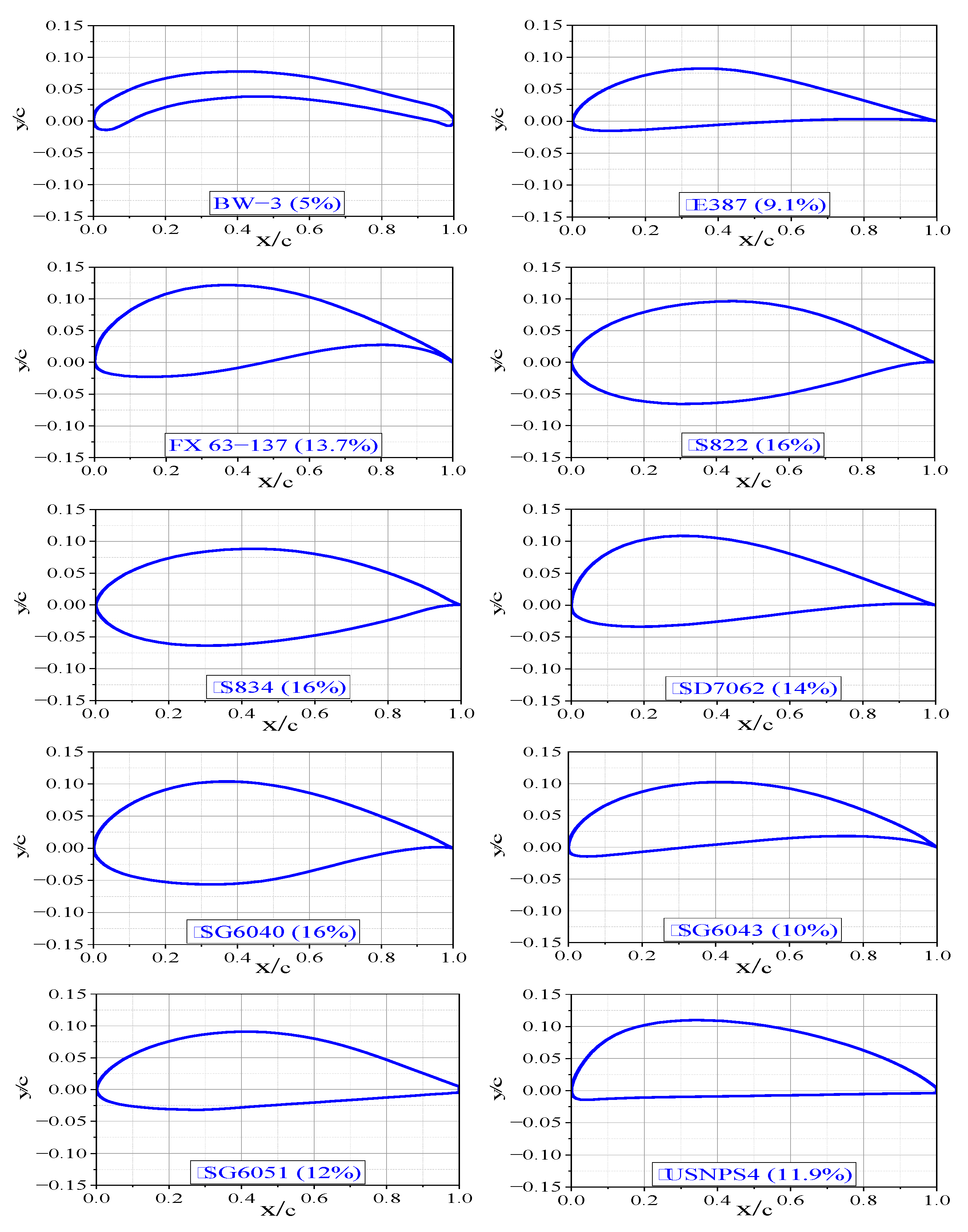
Figure 1. The shape of the selected airfoils.
Machines 10 00687 g001
Figure 2. Velocities on an element of the blade.
Machines 10 00687 g002
Figure 3. Axial and tangential forces on a blade element.
Machines 10 00687 g003
Figure 4. The multi-objective optimization process.
Machines 10 00687 g004
Figure 5. The twist angle and chord length distributions of the turbine in the work of Anderson et al. [45].
Machines 10 00687 g005
Figure 6. The changes of the Cl (top) and Cd (bottom) values of the NACA4412 airfoil [19,26].
Machines 10 00687 g006
Figure 7. Changes in the Cp at different λ values for the present study and the research of Anderson et al. [45].
Machines 10 00687 g007
Figure 8. The twist angle (top) and chord length (bottom) distributions of the blade fitted with the BW-3 airfoil.
Machines 10 00687 g008
Figure 9. Lift-to-drag ratio (top) and Cl (bottom) for the BW-3 airfoil [31].
Machines 10 00687 g009
Figure 10. The maximum lift-to-drag ratio for the selected airfoils [30,31,47].
Machines 10 00687 g010
Figure 11. The distributions of twist (top) and chord (bottom) of the selected airfoils (n = 1).
Machines 10 00687 g011
Figure 12. The torque generated by the blade elements during power generation for n = 1.
Machines 10 00687 g012
Figure 13. The moment of inertia ( J b ) values of the optimized blades (n = 0.8).
Machines 10 00687 g013
Figure 14. The surface area (A) of the selected airfoils.
Machines 10 00687 g014
Figure 15. The distributions of twist (top) and chord (bottom) of the selected airfoils (n = 0.8).
Machines 10 00687 g015
Figure 16. Variations of the startup torque for the selected airfoils (n = 0.8).
Machines 10 00687 g016
Figure 17. Comparison of the performance of the selected airfoils.
Machines 10 00687 g017
Table 1. The specified limits for the design parameters [20].
ParameterMinimumMaximum
Twist, θ(°)−525
Chord, c/R0.010.2
Table 2. The considered input parameters in the DE algorithm.
ParametersValues/Settings
Population2000
Number of generations500
Mutation strategyDE/rand/1
Mutation weighting factor0.8
Crossover operatorUniform
Crossover constant0.1
Table 3. The technical specifications of the considered base turbine [44].
ParametersValues and UnitsParametersValues and Units
P 1000   w U r a t e d 10   m / s
N 3 J G 0.01   kgm 2
R 1.21   m Q r 0.5   Nm
r h 0.125   m ρ b 550   ( kg / m 3 )
ω 450   rpm U s 5   ( m / s )
λ r a t e d 5.71 Airfoil   type SG 6043
Table 4. Optimal values of Cp and Ts for the selected airfoils.
AirfoilWindy Areas (n = 1)Low Wind Areas (n = 0.8)
CpTs (s)CpTs (s)
BW-30.4962.780.4861.82
E3870.5024.870.4853.10
FX 63-1370.4998.440.4893.26
S8220.49513.250.4817.02
S8340.49811.540.4836.87
SD70620.4976.150.4884.49
SG60400.49515.670.4806.02
SG60430.5065.720.4962.89
SG60510.5049.80.4905.13
USNPS40.5035.360.4934.22
Publisher’s Note: MDPI stays neutral with regard to jurisdictional claims in published maps and institutional affiliations.