A Q-Learning-Based Artificial Bee Colony Algorithm for Distributed Three-Stage Assembly Scheduling with Factory Eligibility and Setup Times

Abstract

The assembly scheduling problem (ASP) and distributed assembly scheduling problem (DASP) have attracted much attention in recent years; however, the transportation stage is often neglected in previous works. Factory eligibility means that some products cannot be manufactured in all factories. Although it extensively exists in many real-life manufacturing processes, it is hardly considered. In this study, a distributed three-stage ASP with a $DPm\to 1$ layout, factory eligibility and setup times is studied, and a Q-learning-based artificial bee colony algorithm (QABC) is proposed to minimize total tardiness. To obtain high quality solutions, a Q-learning algorithm is implemented by using eight states based on population quality evaluation, eight actions defined by global search and neighborhood search, a new reward and an adaptive $\epsilon -$greedy selection and applied to dynamically select the search operator; two employed bee swarms are obtained by population division, and an employed bee phase with an adaptive migration between them is added; a new scout phase based on a modified restart strategy is also presented. Extensive experiments are conducted. The computational results demonstrate that the new strategies of QABC are effective, and QABC is a competitive algorithm for the considered problem.

1. Introduction

Scheduling is an important decision-making process in manufacturing and service industries and has been widely studied since 1954. As a typical scheduling problem, ASP is an effective way to balance batch production and production flexibility and has attracted much attention. After the pioneering works of Lee et al. [1] and Potts et al. [2], a number of related works have been obtained. In recent years, Framinan et al. [3] gave a unified notation for ASP and provided a full review of the previous works and future topics. Komaki et al. [4] implemented a consolidated survey of ASP and proposed salient research opportunities.

Two-stage ASP has been widely studied, which consists of a fabrication stage and an assembly stage, and various methods such as exact algorithm, heuristic and meta-heuristics are used to solve the problem. Since meta-heuristic performs better than the exact algorithm ([5,6]) on large-scale scheduling problems and often can produce better results than heuristics, meta-heuristics have become the main approach for solving two-stage ASP, which includes genetic algorithm (GA [7,8]), tabu search (TS [9]), particle swarm optimization (PSO [9]), grey wolf optimizer [10], differential evolution (DE [11]), and imperialist competitive algorithm (ICA [12]) etc.

However, real-life assembly production is typically composed of three sequential stages: fabrication, transportation and assembly. It is unreasonable to ignore the collection and transfer of parts or components, so it is necessary to deal with a three-stage ASP with the transportation stage between the fabrication stage and the assembly stage.

The related results on the three-stage ASP are limited. Christos and George [13] firstly handled the problem and showed that the problem is NP-hard. Hatami et al. [14] presented a mathematical model, a TS and a simulated annealing (SA) for the problem with sequence-dependent setup times (SDST). Maleki-Darounkolaei et al. [15] proposed a meta-heuristic based on SA for the problem with SDST and blocking times. Maleki-Darounkolaei and Seyedi [16] developed a variable neighborhood search (VNS) algorithm and a well-known SA for the same problem. Shoaardebili and Fattahi [17] provided two multi-objective meta-heuristics based on SA and GA to solve the problem with SDST and machine availability. For three-stage ASP with $DPm\to 1$ layout, in which m dedicated parallel machines exist at the fabrication stage and one assembly machine is at the assembly stage, Komaki et al. [18] and Campos et al. [19] presented an improved discrete cuckoo optimization algorithm and a general VNS heuristic, respectively.

With the further development of economic globalization, production is shifted from a single factory to multiple factories, and distributed scheduling in multiple factories has attracted much attention [20,21,22,23,24,25]. DASP is the extended version of ASP in multi-factory environments and a number of works have been obtained on DASP with various processing constraints. Some constructive heuristics and meta-heuristics have been developed for DASP with no-idle [26,27,28,29,30]. Gonzalez-Neira et al. [31] studied a biased-randomized simheuristic for the distributed assembly permutation flowshop problem considering stochastic processing times. Li et al. [32] developed a fuzzy distributed assembly flow shop scheduling problem and presented a novel ICA with empire cooperation. Shao and Shao [33] investigated a distributed assembly blocking flowshop scheduling problem and proposed a constructive heuristic algorithm and a product-based insertion process. They also designed a constructive heuristic and a water wave optimization algorithm with problem-specific knowledge to solve the same problem [34]. Yang and Xu [35] dealt with DASP with flexible assembly and batch delivery and presented seven algorithms using four heuristics, a VNS and two iterated greed (IG). Yang et al. [36] proposed a scatter search-based memetic algorithm to solve the distributed assembly permutation flowshop scheduling problem with no-wait, no-idle and due date constraints. Zhang et al. [37] studied a matrix-cube-based estimation of the distribution algorithm to address the energy-efficient distributed assembly permutation flow-shop scheduling problem.

DASP with setup times is also often considered. Song and Lin [38] presented a genetic programming hyper-heuristic algorithm, and Hatami et al. [39] proposed two constructive heuristics, VNS and IG, for the problem with SDST and makespan. Regarding DASP with a $DPm\to 1$ layout and setup times, Xiong et al. [40] developed a hybrid GA with reduced VNS and a hybrid discrete DE with reduced VNS. Deng et al. [41] presented a mixed integer linear programming model and a competitive memetic algorithm. Zhang and Xing [42] proposed a memetic social spider optimization algorithm by adopting two improvement techniques, the problem-special local search and self-adaptive restart strategy. Lei et al. [43] designed a cooperated teaching-learning-based optimization algorithm with class cooperation.

As stated above, DASP with various processing constraints, such as the no-idle and setup, is considered; however, some constraints, such as factory eligibility, are seldom investigated. Take factory eligibility as an example; this constraint means that not all factories are eligible for each product, that is, at least one product cannot be produced by all factories. This is the extended version of machine eligibility [44,45,46] and often exists in many real-life multi-factory production environments. For example, a large Chinese electronic display company consists of several factories located in different cities in China, and some products cannot be manufactured in all factories. Qin et al. [46] studied a novel integrated production and distribution scheduling problem with factory eligibility and third-party logistics in hybrid flowshops and proposed three heuristics and an adaptive human-learning-based GA; however, DASP with factory eligibility has hardly been investigated; moreover, DASP with factory eligibility and other constraints such as setup times has also hardly been considered. In the real world, multiple factories, factory eligibility and setup times often exist simultaneously, and their considerations can result in a high application value of the obtained schedule; thus, it is necessary to deal with DASP with factory eligibility and setup times.

In recent years, the integration of reinforcement learning (RL) with meta-heuristics has become a new topic, and some results have been produced for production scheduling. Chen et al. [47] solved flexible job shop scheduling by a self-learning GA with a Q-learning algorithm, which is used to adaptively adjust key parameters of GA. Cao et al. [48] presented a cuckoo search (CS) with RL and surrogate modeling for a semiconductor final testing scheduling problem with multi-resource constraints. Cao et al. [49] developed a knowledge-based CS with a knowledge base based on an RL algorithm for flexible job shop scheduling with sequencing flexibility. In these two papers, the parameters of CS are also adjusted by RL. Oztop et al. [50] dealt with a no-idle flowshop scheduling problem by using a novel general VNS with Q-learning algorithm used to determine the parameters of VNS. Ma and Zhang [51] provided an improved ABC algorithm based on a Q-learning algorithm. Lin et al. [52] applied a Q-learning-based hyper-heuristic (QHH) algorithm to solve a semiconductor final testing scheduling problem. In QHH, a Q-learning algorithm is used to autonomously select a heuristic from a heuristic set. Karimi-Mamaghan et al. [53] proposed a novel efficient IG algorithm for the permutation flowshop scheduling problem, which can adaptively select the perturbation operators using the Q-learning algorithm. The above integrations of RL and meta-heuristics are mainly used to adaptively adjust parameter settings or select a search operator [54,55]. As a result, the performance of the meta-heuristic can be improved, and thus, it is an effective way to add RL into a meta-heuristic for scheduling problems such as DASP with factory eligibility.

As shown above, meta-heuristics, including GA, PSO and VNS, are frequently applied to solve ASP and DASP. As the main method for production scheduling, ABC has been successfully applied to cope with various production scheduling problems in a single factory [56,57,58,59,60] and multiple factories [61,62,63,64,65]; however, ABC is seldom used to solve DASP. Compared with some meta-heuristics such as GA, ABC has some features such as simplicity and ease of implementation; on the other hand, ABC has successful applications in single factory scheduling and distributed scheduling [64,65,66,67] with permutation-based representation, and the solution of DASP is also represented as a permutation of products. ABC is suitable for solving DASP; moreover, the RL algorithm can be integrated easily with ABC because of its above features. As a result, the performance of ABC can be improved effectively, and thus, it can be concluded from the above analyses that it is beneficial to apply ABC to solve DASP by its integration with RL [68].

In this study, transportation stage, factory eligibility and setup times are adopted in a distributed three-stage ASP, and an effective path is given to integrate the Q-learning algorithm and ABC. The main contributions can be summarized as follows. (1) A distributed three-stage ASP with $DPm\to 1$ layout, factory eligibility and setup times is considered. (2) A Q-learning-based artificial bee colony (QABC) is proposed to minimize total tardiness. A Q-learning algorithm is implemented by using eight states based on population quality evaluation, eight actions defined by global search and neighborhood search, a new reward and an adaptive $\epsilon -$greedy selection. Unlike the previous works [47,48,49,50], the Q-learning algorithm is applied to dynamically select a search operator. Population division, the employed bee phase with adaptive migration and a new scout phase based on a modified restart strategy are also added. (3) Extensive experiments are conducted to test the performances of QABC by comparing it with other methods from the literature. Computational results demonstrate that the usage of new strategies, including Q-learning, is effective and efficient, and QABC can provide promising results for the considered problem.

The remainder of the paper is organized as follows. The problem description is given in Section 2 followed by an introduction to ABC and Q-learning in Section 3. Section 4 shows the proposed QABC for the problem. Numerical experiments on QABC are reported in Section 5, the conclusions are summarized in the final section and some topics of future research are provided.

2. Problem Description

Distributed three-stage ASP with $DPm\to 1$ layout, factory eligibility, and setup times is described as follows. Notations used for this problem are shown in Table 1.

Table 1. A summary of notations.

Indexes and Parameters	Description
$i,j$	Product index $i,j\in \{1,2,\cdots ,n\}$
k	Processing machine and product indexes $k\in \{1,2,\cdots ,m\}$
f	Factory index $f\in \mathit{F}$
$\mathit{F}$	Factory set $\mathit{F}=\{1,2,\cdots ,F\}$
n	Number of products
m	Number of fabrication machines and components of each product
F	Number of factories
${\mathit{F}}_i$	Feasible factory set of product i, ${\mathit{F}}_i\subseteq \mathit{F}$
$M_{kf}$	The kth fabrication machine of factory f
$T{M}_f$	Transportation machine of factory f
$A{M}_f$	Assembly machine of factory f
$p{t}_{ikf}$	Processing time of its kth component on machine $M_{kf}$
$t{t}_{if}$	Transportation time on $T{M}_f$
$a{s}_{if}$	Assembly time on $A{M}_f$
$sp{t}_{ikf}$	Setup time of the kth component of product i on $M_{fk}$
$st{t}_{if}$	Setup time of product i on $T{M}_f$
$sa{s}_{if}$	Setup time of product i on $A{M}_f$
$d_i$	Due date of product i
$C_i$	The completion time of product i
$T_i$	Tardiness of product i, $T_i=max\left\{C_i-d_i,0\right\}$
$TT$	Total tardiness of all products

There are n products and F factories in a factory set $\mathit{F}$. Factory eligibility means that there exists an available factory set ${\mathit{F}}_i$ for product i, ${\mathit{F}}_i\subseteq \mathit{F}$. Each factory f has m dedicated parallel machines $M_{1f},M_{2f},\cdots ,M_{mf}$ for fabrication, a transportation machine $T{M}_f$ and an assembly machine $A{M}_f$. With respect to $T{M}_f$, it just works in a factory f, suppose that $T{M}_f$ has sufficient capacity so that all components of any products can be transferred at one time. In a transportation, $T{M}_f$ moves components of just one product i from the fabrication machine of the last finished component to $A{M}_f$. All components of each product are transported by $T{M}_f$ once.

Each product has m components. When product i is allocated into factory $f\in {\mathit{F}}_i$, its m components are first processed on $M_{1f},M_{2f},\cdots ,M_{mf}$ at the fabrication stage, and then they are collected by $T{M}_f$ and transferred to $A{M}_f$ at the assembly stage; finally, the product is obtained by assembling its all components.

Setup time is anticipatory and can start when a machine is available, which is required for three stages. For production i transferred by $T{M}_f$, its setup time $st{t}_{if}$ is used to load and unload product i.

Factory eligibility indicates that not all factories are eligible for each product, that is, at least one product i has a set ${\mathit{F}}_i\subset \mathit{F}$.

All products can be produced at time 0; each machine can fabricate, transport or assemble at most one product at a time; each product can be fabricated, transported or assembled at most one machine at a time; no interruption and breakdowns are considered; once a product is assigned to a factory, it cannot be transferred to another factory.

The problem can be divided into factory assignment sub-problem and scheduling sub-problem. There are strong coupled relations between the two sub-problems. Factory assignment notably affects the results of the scheduling sub-problem, and optimal solutions can be obtained after the solutions to the two sub-problems are effectively combined.

The goal of the problem is to minimize total tardiness when all constraints are met.

$$TT={\sum }_{i=1}^n{T}_i$$

(1)

An illustrative example with six products ($n=6$), three factories ($F=3$) and three machines ($m=3$) at the fabrication stage of each factory is shown in Table 2. For factory set $\mathit{F}=\{1,2,3\}$, product i can be produced by the factory in ${\mathit{F}}_i\subseteq \mathit{F}$, ${\mathit{F}}_1=\left\{2\right\}$, ${\mathit{F}}_2=\{1,3\}$, ${\mathit{F}}_3=\{1,2\}$, ${\mathit{F}}_4=\{1,2,3\}$, ${\mathit{F}}_5=\left\{3\right\}$, ${\mathit{F}}_6=\{1,2,3\}$. “—” For example, in ${\mathit{F}}_1=\left\{2\right\}$, product 1 cannot be assigned to factories 1 and 3, then $p{t}_{112}=31$, $p{t}_{122}=26$, and so on. A Gantt chart of a schedule of the example is shown in Figure 1, $T_1=6$, $T_2=0$, $T_3=37$, $T_4=0$, $T_5=0$, $T_6=34$, total tardiness of factory 1, 2, and 3 is 37, 6, 34, respectively, and the corresponding $TT$ is 77.

Table 2. An illustrative example.

i	1	2	3	4	5	6
${\mathit{F}}_i$	{2}	{1, 3}	{1, 2}	{1, 2, 3}	{3}	{1, 2, 3}
$p{t}_{i1f}$	—, 31, —	52, —, 84	14, 11,—	88, 38, 66	—, —, 55	18, 27, 64
$p{t}_{i2f}$	—, 26, —	54, —, 67	21, 77,—	30, 27, 82	—, —, 97	51, 79, 8
$p{t}_{i3f}$	—, 60, —	54, —, 16	39, 9,—	64, 50, 42	—, —, 30	10, 66, 47
$t{t}_{if}$	—, 22, —	65, —, 57	39, 79,—	16, 17, 86	—, —, 42	13, 95, 65
$a{t}_{if}$	—, 45, —	47, —, 51	89, 51,—	88, 68, 3	—, —, 41	88, 59, 50
$sp{t}_{i1f}$	—, 9, —	19, —, 19	7, 6,—	19, 19, 19	—, —, 3	17, 4, 18
$sp{t}_{i2f}$	—, 17, —	4, —, 8	10, 2,—	12, 11, 14	—, —, 7	13, 18, 19
$sp{t}_{i3f}$	—, 18, —	17, —, 7	20, 20,—	4, 15, 6	—, —, 7	20, 4, 16
$st{t}_{if}$	—, 7, —	8, —, 9	13, 16,—	11, 2, 8	—, —, 7	7, 4, 19
$sa{t}_{if}$	—, 12, —	13, —, 5	9, 15,—	15, 3, 11	—, —, 2	20, 10, 8
$d_i$	204	357	150	245	228	448

Figure 1. A schedule of the example.

3. Introduction to ABC and Q-Learning

In this study, ABC and an RL algorithm named Q-learning are integrated together; thus, we introduce ABC and the Q-learning algorithm.

3.1. ABC

In ABC, a feasible solution to the problem is represented by a food source, and a search agent is represented by a bee. All bees are categorized into three groups: employed bees, onlooker bees and scouts. In general, the employed bee tries to exploit a food source, the onlooker bee waits in the hive to make a decision of choosing a food source, and the scout carries out a random search for a new food source.

ABC begins with a randomly generated initial population P with N solutions, and then three phases called employed bee phase, onlooker bee phase, and scout phase are executed sequentially.

In the employed bee phase, each employed bee produces a candidate source $x_b^{{}^{\prime }}$ from $x_b=\{x_{b1},x_{b2},\cdots ,x_{bD}\}$$,x_b\in P$.

$$x_{b\omega }^{{}^{\prime }}=x_{b\omega }+\varphi (x_{b\omega }-x_{c\omega })$$

(2)

where D is the number of dimensions, $\varphi$ is a real random number in the range $[-1,1]$, and $x_c\in P$ is a randomly selected solution, $b,c\in \{1,2,\cdots ,N\}$, $b\ne c$, $\omega \in \{1,2,\cdots ,D\}$.

A greedy selection is applied: if $fit\left(x_b^{{}^{\prime }}\right)<fit\left(x_b\right)$, then $x_b^{{}^{\prime }}$ substitutes for $x_b$, where $fit\left(x_b\right)$ denotes fitness of $x_b$.

In the onlooker bee phase, the onlooker bee chooses a food source by roulette selection based on the probability $pro{b}_b$.

$$pro{b}_b=fit\left(x_b\right)/\phantom{fit\left(x_i\right){\sum }_{y\in P}fit\left(y\right)}\sum _{v=1}^{N}fit\left(x_v\right)$$

(3)

Once an onlooker bee selects a food solution $x_b$, a new solution $x_b^{{}^{\prime }}$ is obtained, and then the above greedy selection is applied to decide if $x_b$ can be replaced with $x_b^{{}^{\prime }}$.

In the above two phases, a $tria{l}_b$ is computed for each ${\mathbf{x}}_b$. Initially, $tria{l}_b=0$. If the newly obtained $x_b^{{}^{\prime }}$ cannot update ${\mathbf{x}}_b$, $tria{l}_b=tria{l}_b+1$; otherwise, $tria{l}_b=0$.

In the scout phase, if $tria{l}_b$ of a food source exceeds a threshold $Limit$, the corresponding employed bee will turn into a scout, which randomly produces a solution to substitute for the food source.

3.2. Introduction to Q-Learning Algorithm

RL is a learning approach that can be applied to a wide variety of complex problems. RL has been extensively considered and has been successfully applied to solve many problems [47,48,49,50,51,69,70].

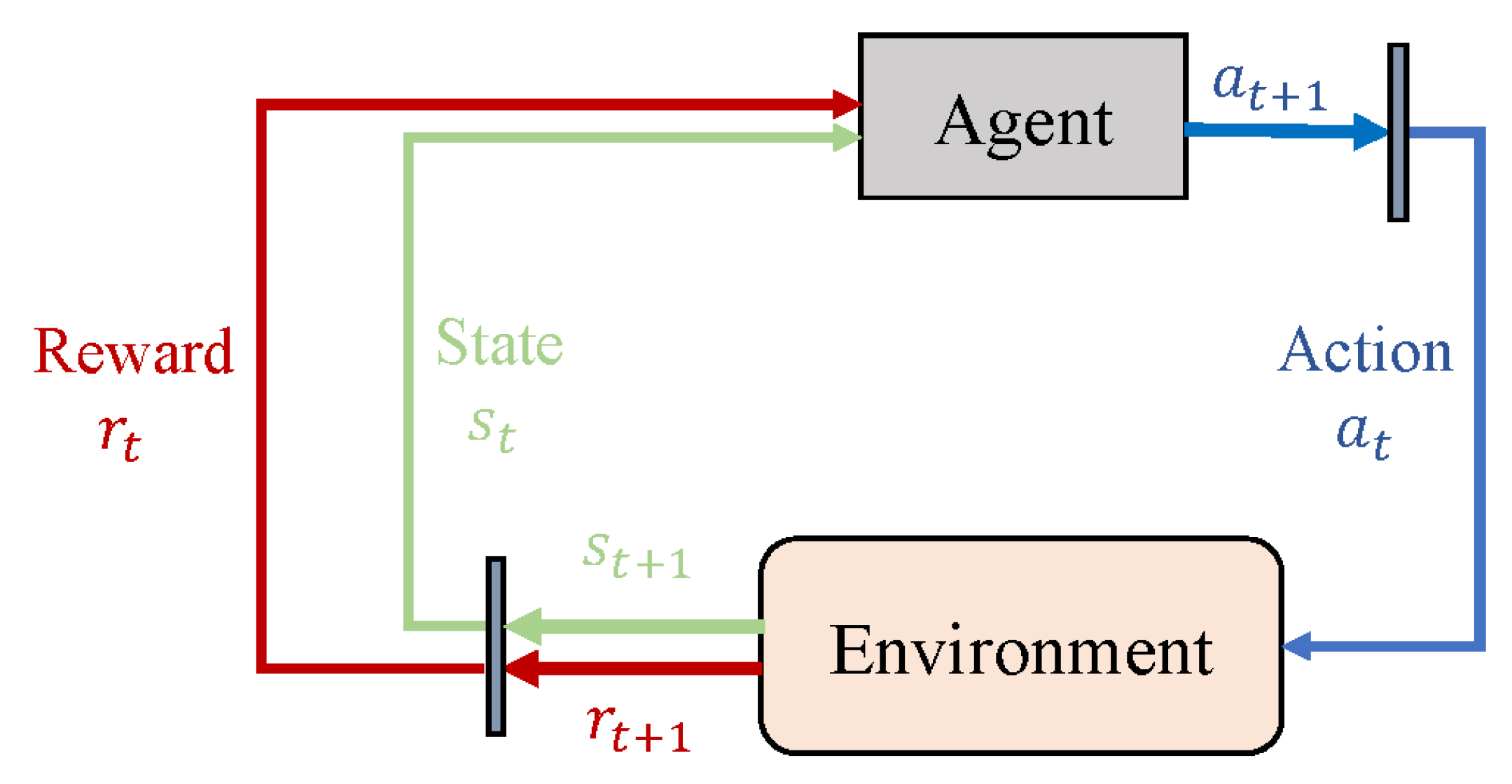
The Q-learning algorithm [71] is the most commonly used model-free RL algorithm. It provides a learning capability for the intelligence system in the Markov environment to select the optimal action using the experienced action. The main components of Q-learning include a learning agent, an environment, states, actions, and rewards. The illustration plot is shown in Figure 2. The Q-learning algorithm has a simple structure and is implemented easily. It has been successfully integrated with meta-heuristics such as GA, CS and QHH for production scheduling [47,48,52]. Its simplest form is defined by

$$Q_{}\left(s_t,a_t\right)\leftarrow Q\left(s_t,a_t\right)+\alpha \left[r_{t+1}+\gamma \underset{a}{max}Q\left(s_{t+1},a\right)-Q\left(s_t,a_t\right)\right]$$

(4)

where $\alpha$ is the learning rate, $\gamma$ indicates the discount factor, $r_{t+1}$ is the reward received from the environment by taking the $a_t$ of $s_t$, and $\underset{a}{max}Q(s_{t+1},a)$ represents the biggest Q value in the Q-table at state $s_{t+1}$.

Figure 2. An illustration of Q-learning.

Action selection is performed based on the Q-table. Initially, all elements of the Q-table are zero, which means that the agent does not have any learning experience. $\epsilon -$greedy is often used and expressed as follows. If a random number $rand<\epsilon$, then randomly select an action a; otherwise, select an action a that maximizes the Q values, that is, $a=arg{max}_{a^{\prime }}Q\left(s_t,a^{\prime }\right)$.

4. QABC for Distributed Three-Stage ASP with Factory Eligibility and Setup Times

This study contributes an effective integration of the Q-learning algorithm and ABC to implement the dynamical selection of the search operator. Moreover, two employed bee swarms are used for population division, and a new scout phase based on a modified restart strategy is also applied. The details of QABC are shown below.

4.1. Representation and Search Operators

4.1.1. Solution Representation

Because the problem has two sub-problems, a two-string representation is used, in which a solution is denoted by a factory assignment string $[{\theta }_1$, ${\theta }_2$, ⋯, ${\theta }_n]$ and a scheduling string $[q_1$, $q_2$, ⋯, $q_n]$, where factory ${\theta }_i$ is allocated for product i, ${\theta }_i\in {\mathit{F}}_i$ and $q_i$ is a real number in $[0,1]$ and corresponds to product i.

The scheduling string is a random key one, so suppose that products i, $i+1$, ⋯, j are manufactured in the same factory, that is, ${\theta }_i$ = ${\theta }_{i+1}$= ⋯ = ${\theta }_j$, product permutation is determined after all $q_l$ are sorted in ascending order, $l\in [i,j]$, $i<j$. If $q_i=q_j$, then product i will be placed before product j because j is greater than i.

The decoding procedure is shown in Algorithm 1. For the example in Table 2, a possible solution is composed of factory assignment string $[2$, 3, 1, 2, 3, $1]$ and scheduling string $[0.98$, $0.43$, $0.32$, $0.21$, $0.72$, $0.67]$. For factory 1, products 3 and 6 are assigned to it in terms of factory assignment string, their permutation [3, 6] is obtained because $q_3<q_6$, that is, product 3 starts followed by product 6.  Take product 3 as an example; three components of it are first processed on $M_{1f},M_{2f},M_{3f}$, and then they are collected by $T{M}_f$ and transferred to $A{M}_f$ to assemble them. The corresponding schedule is illustrated in Figure 1.

Algorithm 1: Decoding procedure

Input: factory assignment string $[{\theta }_1$, ${\theta }_2$, ⋯, ${\theta }_n]$; scheduling string $[q_1$, $q_2$, ⋯, $q_n]$

Output: Permutations of all factories

1: for$f=1$ to F do

2:    Find all products allocated to factory f according to factory assignment string

3:    Determine permutation of all products in factory f by sorting $q_l$ in ascending order

4:    Start with the first product on the permutation, handle the fabrication of all of its components, transfer all of its components to $A{M}_f$ and assemble them.

5: end for

4.1.2. Search Operators

In this study, a search operator is made up of a global search between two solutions, reassignment, inversion and neighborhood search.

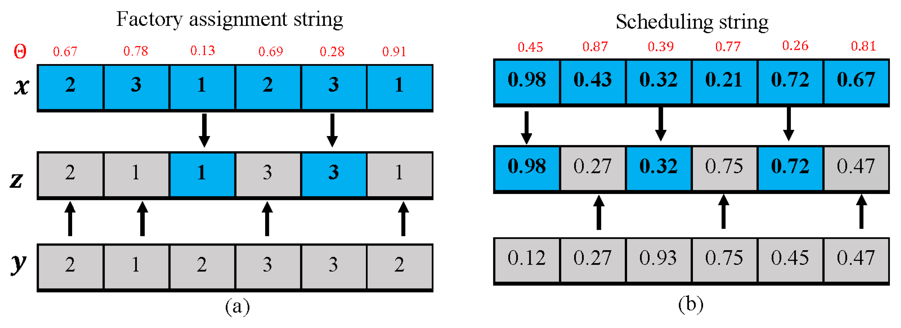
A global search between solutions $x,y$ is shown below. Solution z is produced by a uniform crossover of both the factory assignment string and scheduling string of $x,y$, and greedy selection is applied: if z is better than x, then x is replaced with z. Figure 3 describes the process of a uniform crossover of the above two strings. In Figure 3a, a string $\Theta$ of random numbers [0.67, 0.78, 0.13, 0.69, 0.28, 0.91] is obtained, and then, a new factory assignment string $[2,1,1,3,3,1]$ is produced by elements in string $\Theta$. For example, the first element is $0.67>0.5$, and the first gene of z is selected from y; the third element is $0.13\le 0.5$, and the third gene of z is from x.

Figure 3. Example of a global search. (a) Factory assignment string; (b) Scheduling string.

Total tardiness is related to each factory, so uniform crossover is used and simultaneously acts on two strings of x, y.

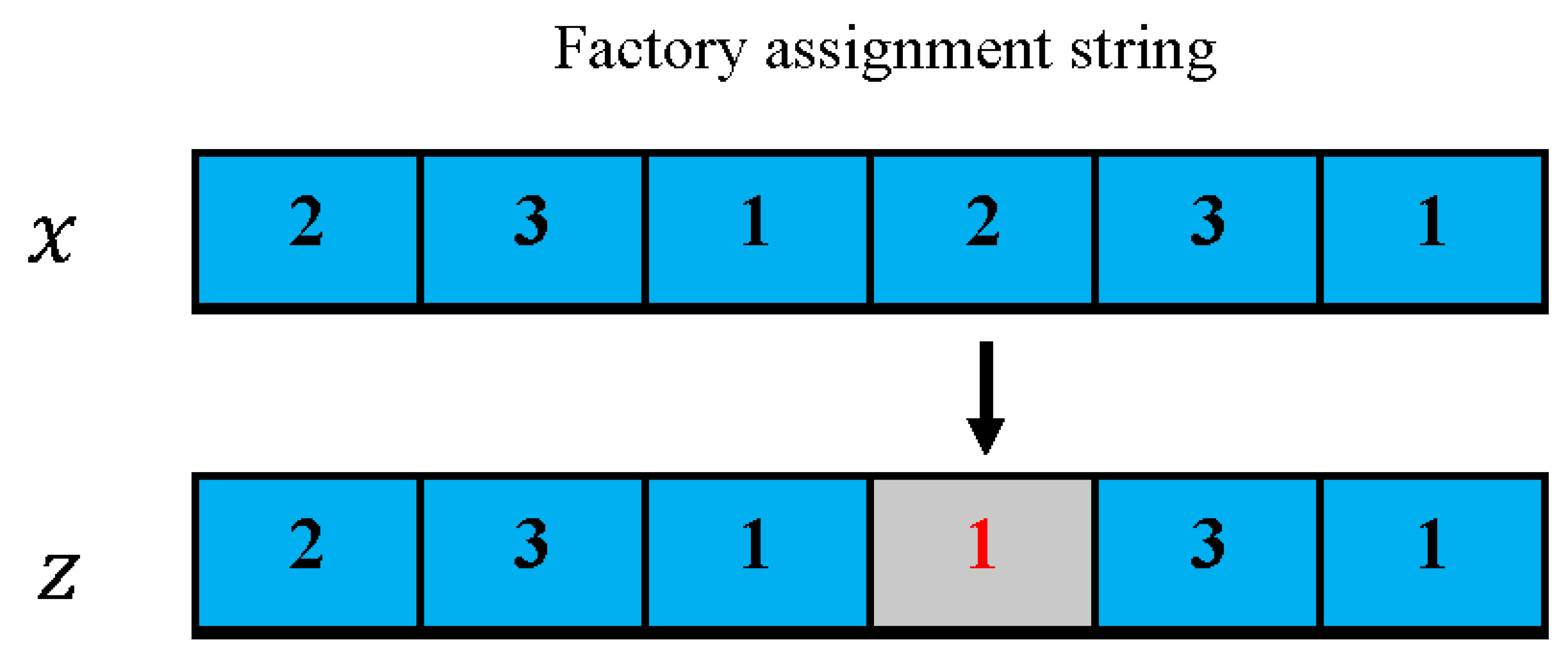
The reassignment operator acts on a factory assignment string of a solution x in the following way: randomly select $\beta =⌈\mu \times n⌉$ genes, and then each chosen gene ${\theta }_l$ is displaced by a randomly decided factory in ${\mathit{F}}_l$, a new solution z is obtained, and a greedy selection is executed, where $\mu$ is a random decimal in the range (0, 1], and $⌈u⌉$($\ge u$) indicates the closest integer to u. An example of a reassignment operator is shown in Figure 4. If $\mu$ = 0.45, $\beta =3$, three products 2, 4, and 6 are randomly selected. ${\theta }_2$ = 1 can be obtained, which is randomly chosen from ${\mathit{F}}_2$. ${\theta }_4=3$ and ${\theta }_6=2$ are generated similarly.

Figure 4. Example of reassignment operator.

Inversion is described as follows. For scheduling string of a solution x, randomly decide ${\tau }_1,{\tau }_2$, ${\tau }_1<{\tau }_2$ and invert genes between positions ${\tau }_1$ and ${\tau }_2$. A new solution z is produced, and greedy selection is complete.

Eight neighborhood structures ${\mathcal{N}}_1-{\mathcal{N}}_8$ are used to construct a neighborhood search. The factory with maximum total tardiness is defined as the critical factory $f^{*}$. The position is decided based on the product permutation of the factory.

Neighborhood structure ${\mathcal{N}}_1$ is described below. Stochastically select a product i from the factory $f^{*}$, insert i into a randomly decided position of the factory $f^{*}$, and reassign $q_i$ of each product according to the product permutation of the factory $f^{*}$. For the above solution of the example, the critical factory $f^{*}$ is 1, product 3 is inserted into the position of product 6, and a new permutation is $6,3$, so $q_6=0.32$ and $q_3=0.67$.

When a randomly chosen factory substitutes for the factory $f^{*}$ in ${\mathcal{N}}_1$, ${\mathcal{N}}_2$ is obtained. ${\mathcal{N}}_3$ is shown as follows. Swap two randomly selected products from the factory $f^{*}$. ${\mathcal{N}}_4$ differs from ${\mathcal{N}}_3$ in that a stochastically chosen factory is used.

${\mathcal{N}}_5$ acts on the factory $f^{*}$ in the following way: a product i with $T_i>0$ is randomly selected from the factory $f^{*}$, suppose that i is on the position ${\tau }_1$ of product permutation of the factory $f^{*}$, insert i into a randomly decided position ${\tau }_2<{\tau }_1$. When a randomly selected factory is substituted for factory $f^{*}$ in ${\mathcal{N}}_5$, ${\mathcal{N}}_6$ is produced.

${\mathcal{N}}_7$ is shown below. Randomly find a product i with $T_i>0$ from the factory $f^{*}$ and stochastically choose a factory $f\in {\mathit{F}}_i$, remove i from the critical factory and insert it into a randomly decided position of factory f. An example of ${\mathcal{N}}_7$ is shown in Figure 5, in which $f^{*}=2$, $i=4$ with $T_4>0$ is selected stochastically, and ${\theta }_4$ is replaced by another factory 1 that is randomly chosen from ${\mathit{F}}_4$.

Figure 5. Example of $N_7$.

The above neighborhood structures of the critical factory are proposed because of the following feature of the problem: a new position of product i in critical factory $f^{*}$ or a movement of product i from factory $f^{*}$ to another factory is very likely to diminish total tardiness.

Seven neighborhood searches are constructed by different combinations of neighborhood structures. $N{S}_1$ contains four neighborhood structures ${\mathcal{N}}_1$, ${\mathcal{N}}_3$, ${\mathcal{N}}_5$, ${\mathcal{N}}_7$ related to the critical factory $f^{*}$. $N{S}_2$ consists of ${\mathcal{N}}_2$, ${\mathcal{N}}_4$, ${\mathcal{N}}_6$, ${\mathcal{N}}_8$. In $N{S}_3$, six insertion-related neighborhood structures ${\mathcal{N}}_1$, ${\mathcal{N}}_2$, ${\mathcal{N}}_5$, ${\mathcal{N}}_6$, ${\mathcal{N}}_7$, ${\mathcal{N}}_8$ are applied. $N{S}_4$ is composed of two swap-based neighborhood structures ${\mathcal{N}}_3$, ${\mathcal{N}}_4$.

$N{S}_5$ is established by ${\mathcal{N}}_1$, ${\mathcal{N}}_2$, ${\mathcal{N}}_3$ and ${\mathcal{N}}_4$. ${\mathcal{N}}_5$, ${\mathcal{N}}_6$, ${\mathcal{N}}_7$, and ${\mathcal{N}}_8$ are used in $N{S}_6$. $N{S}_7$ has all eight structures for a comprehensive effect.

The procedure of each $N{S}_{\phi }$ is given in Algorithm 2. Seven search operators are defined, each of which is composed of a global search, reassignment, inversion and $N{S}_{\phi }$, $\phi \in \{1,2,\cdots ,7\}$. $w_{\phi }$ is the number of neighborhood structure in $N{S}_{\phi }$, $w_1=4$, $w_2=4$, $w_3=6$, $w_4=2$, $w_5=4$, $w_6=4$, $w_7=8$.

Algorithm 2: $N{S}_{\phi }$

Input:x, $R_1$

Output: updated solution x

1: let $Iter=0$

2: while $Iter<R_1$do

3:     randomly decide a usage sequence of all neighborhood

4:     structures of $N{S}_{\phi }$

5:     suppose that the obtained sequence is $g_1,g_2,\cdots ,g_{w_{\phi }}$

6:     let $h=1$

7:     while $h\le w_{\phi }$ do

8:         produce a new solution $z\in N_{g_h}\left(x\right)$

9:         if $fit\left(z\right)<fit\left(x\right)$ then

10:            $x=z$

11:         else

12:            $h=h+1$

13:         end if

14:         $Iter=Iter+1$

15:     end while

16: end while

17: return updated solution x

4.2. Q-Learning Algorithm

In this study, the Q-learning algorithm is integrated with ABC to dynamically select the search operator. To realize the above purpose, population evaluation results are used to describe state $s_t$, the search operator described above is applied to depict action $a_t$, and, as a result, action selection can result in a dynamical selection of the search operator.

4.2.1. State and Action

Three indices are used to evaluate population quality, which are $tria{l}^{*}$ of elite solution $x^{*}$, evolution quality $Ev{o}^t$ of population P and diversity index $D^t$. Initially, $tria{l}^{*}=0$, if elite solution $x^{*}$ is updated, then $tria{l}^{*}=0$; otherwise, $tria{l}^{*}=tria{l}^{*}+1$, where $tria{l}^{*}$ is defined similarly to $tria{l}_i$ in Section 3.1.

$$Ev{o}^t=\frac{{\sum }_{x_i\in P}{u}_i^t}{N}$$

(5)

$$D^t=\frac{{\sum }_{x_i\in P}{v}_i^t/\phantom{v_{i}N-1}N-1}{N}$$

(6)

where $u_i^t=1$ if $tria{l}_i=0$ on generation t and 0 otherwise; $v_i^t=\left|\left\{x_j\right|j\ne i,fit\left(x_j\right)\ne fit\left(x_i\right)\}\right|$ on generation t.

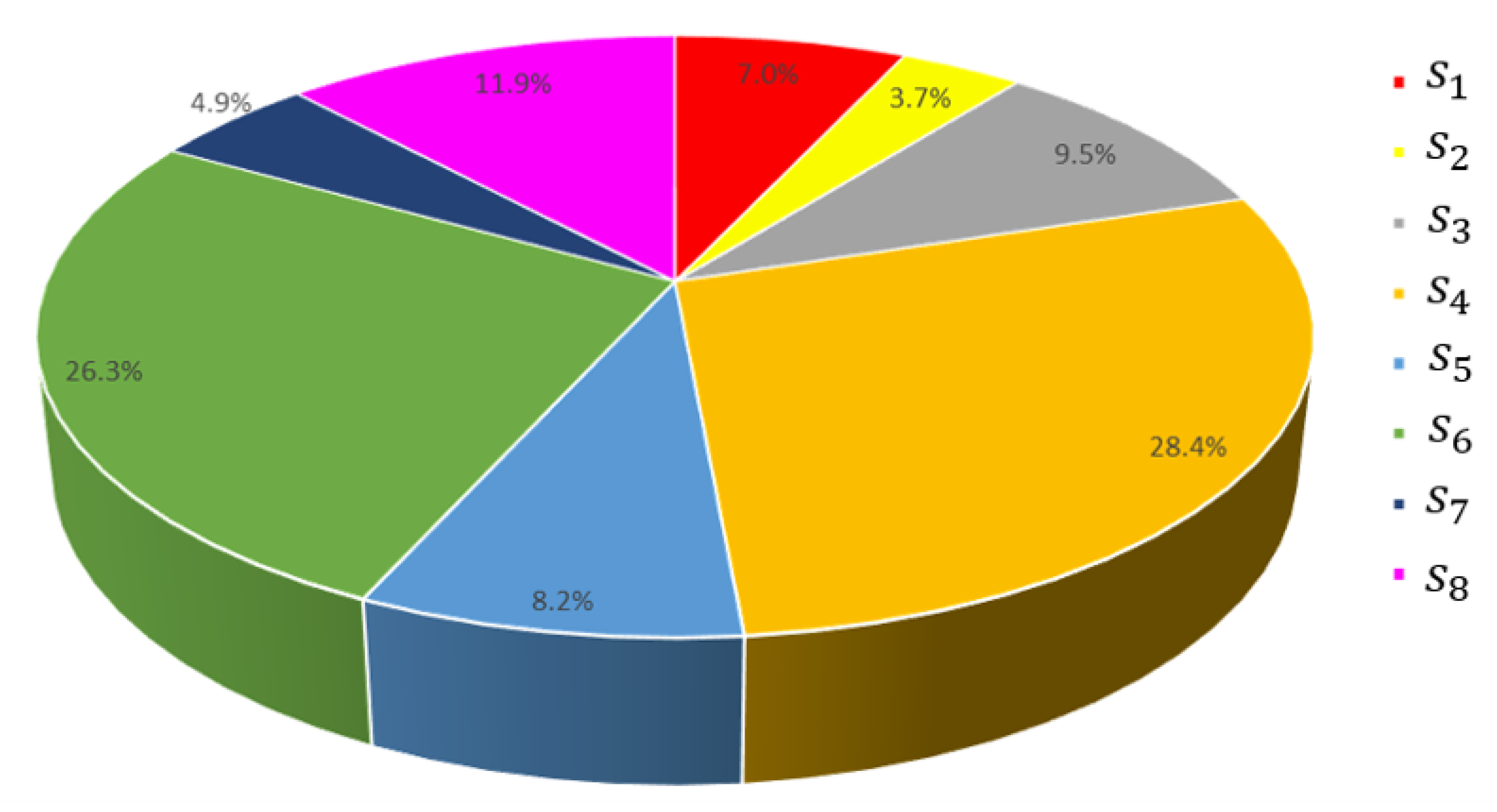
Eight states are depicted by using three indices, as shown in Table 3. $tria{l}^{*}=0$ means that the elite solution $x^{*}$ is updated on generation t. Elite solution $x^{*}$ does not deteriorate because of greedy selection, so $tria{l}^{*}$ may be 0 or positive, ${\mu }_1$, ${\mu }_2$ are integers, ${\mu }_2>{\mu }_1$. ${\mu }_1=20$ and ${\mu }_2=50$ are obtained by experiments. For $Ev{o}^t$ and $D^t$, two cases exist, which are $Ev{o}^t\ge D^t$ and $Ev{o}^t<D^t$.

Table 3. The eight state representations.

State	State Description
$s_1$	$tria{l}^{*}=0$ and $Ev{o}^t\ge D^t$
$s_2$	$tria{l}^{*}=0$ and $Ev{o}^t<D^t$
$s_3$	$0<tria{l}^{*}\le {\mu }_1$ and $Ev{o}^t\ge D^t$
$s_4$	$0<tria{l}^{*}\le {\mu }_1$ and $Ev{o}^t<D^t$
$s_5$	${\mu }_1<tria{l}^{*}\le {\mu }_2$ and $Ev{o}^t\ge D^t$
$s_6$	${\mu }_1<tria{l}^{*}\le {\mu }_2$ and $Ev{o}^t<D^t$
$s_7$	$tria{l}^{*}>{\mu }_2$ and $Ev{o}^t\ge D^t$
$s_8$	$tria{l}^{*}>{\mu }_2$ and $Ev{o}^t<D^t$

For the instance of $250\times 5\times 20$ depicted in Section 5, Figure 6 shows the percentage of occurrence in four cases of $tria{l}^{*}$ and two cases of $Ev{o}^t$ and $D^t$ in the whole search process of QABC, and Figure 7 presents a pie chart of the percentage of the eight states. It can be found that all states exist in the search process of QABC, so it is reasonable to set eight states.

Figure 6. Four cases on $tria{l}^{*}$ and two cases of $Ev{o}^t$ and $D^t$.

Figure 7. Percentages of eight states.

In QABC, population P is divided into two employed bee swarms $E{B}_1$, $E{B}_2$ and an onlooker bee swarm $OB$. Population division is shown below. Initially, $E{B}_1$, $E{B}_2$, $OB$ are empty. The dividing steps are shown below. Randomly select $⌈{\beta }_1\times N⌉$ solutions from population P and add them into $E{B}_1$, then stochastically choose $⌈{\beta }_2\times N⌉$ solutions from the remaining part of P and include them in $E{B}_2$; finally, $OB$ consists of the remaining solutions in P. ${\beta }_1$, ${\beta }_2\in [0.25,0.4]$ based on experiments.

Seven search operators are directly defined as actions $a_1$, $a_2$, ⋯, $a_7$. $a_{\phi }$ is composed of global search, reassignment, inversion and $N{S}_{\phi }$. Once action $a_{\phi }$, $\phi \le 7$ is chosen, it acts on $E{B}_1$, $E{B}_2$ and $OB$. Action $a_8$ is defined by randomly selecting a search operator $a_{\phi },\phi \le 7$ for $E{B}_1$, $E{B}_2$ and $OB$, respectively, so when $a_8$ is selected, $E{B}_1$, $E{B}_2$ and $OB$ may apply different search operators.

4.2.2. Reward and Adaptive Action Selection

Elite solution $x^{*}$ is the output of QABC, and its improvement is very important for QABC. When $tria{l}^{*}=0$, that is, $x^{*}$ is updated, a positive reward should be given; moreover, the bigger the $Ev{o}^t+D^t+Im{e}^t$ is, the bigger the reward is. When $tria{l}^{*}>0$, the elite solution is kept invariant; in this case, a negative reward should be added. Based on the above analyses, reward $r_{t+1}$ is defined by

$$r_{t+1}=\left\{\begin{array}{cc}{e}^{\left(4\times Im{e}^{t+1}+Ev{o}^{t+1}+D^{t+1}\right)/\phantom{\left(4\times Im{e}^{t+1}+Ev{o}^{t+1}+D{i}^{t+1}\right)3}3}\hfill & iftria{l}^{*}=0\hfill \\ -e^{Ev{o}^{t+1}+D{i}^{t+1}}\hfill & otherwise\end{array}\right.$$

(7)

Let $A,B$ indicate $fit\left(x^{*}\right)$ on generations t and $t+1$, respectively,

$$Im{e}^{t+1}=(A-B)/A$$

(8)

For $\epsilon$-greedy action selection, the learner will explore with the probability $\epsilon$ and exploit the historical experience with the probability of $1-\epsilon$ by choosing the action with the highest Q value, where $\epsilon$ plays a key role in the trade-off between exploration and exploitation, and some adaptive methods are used [72,73].

In this study, a new adaptive $\epsilon$-greedy action selection is proposed, where $\epsilon$ is adaptively changed with $tria{l}^{*}$ and the current selected action $a_t$,

$$\epsilon \leftarrow \left\{\begin{array}{cc}max\left\{{\epsilon }_0,\epsilon \times \left(1-\epsilon \right)\right\}\hfill & \begin{array}{c}iftria{l}^{*}=0and\hfill \\ a_t=arg\underset{a}{max}Q\left(s_t,a\right)\hfill \\ ortria{l}^{*}>0and\hfill \\ a_t\ne arg\underset{a}{max}Q\left(s_t,a\right)\hfill \end{array}\hfill \\ min\left\{\epsilon \times \left(1+\epsilon \right),1-{\epsilon }_0\right\}\hfill & \begin{array}{c}iftria{l}^{*}>0and\hfill \\ a_t=arg\underset{a}{max}Q\left(s_t,a\right)\hfill \\ ortria{l}^{*}=0and\hfill \\ a_t\ne arg\underset{a}{max}Q\left(s_t,a\right)\hfill \end{array}\end{array}\right.$$

(9)

where ${\epsilon }_0=0.01$. Obviously, $\epsilon \in [0.01,0.99]$.

If $tria{l}^{*}=0$ and $a_t=\underset{a}{max}Q(s_t,a)$, that is, action $a_t$ with the biggest $Q(s_t,a)$ leads to new $x^{*}$, in this case, $\epsilon$ should be reduced to enlarge the probability of exploitation; if $tria{l}^{*}=0$ and $a_t\ne \underset{a}{max}Q(s_t,a)$, that is, a randomly chosen $a_t$ results in a new $x^{*}$, then $\epsilon$ should increase for a larger probability of exploration. Two other cases can be explained in the same way.

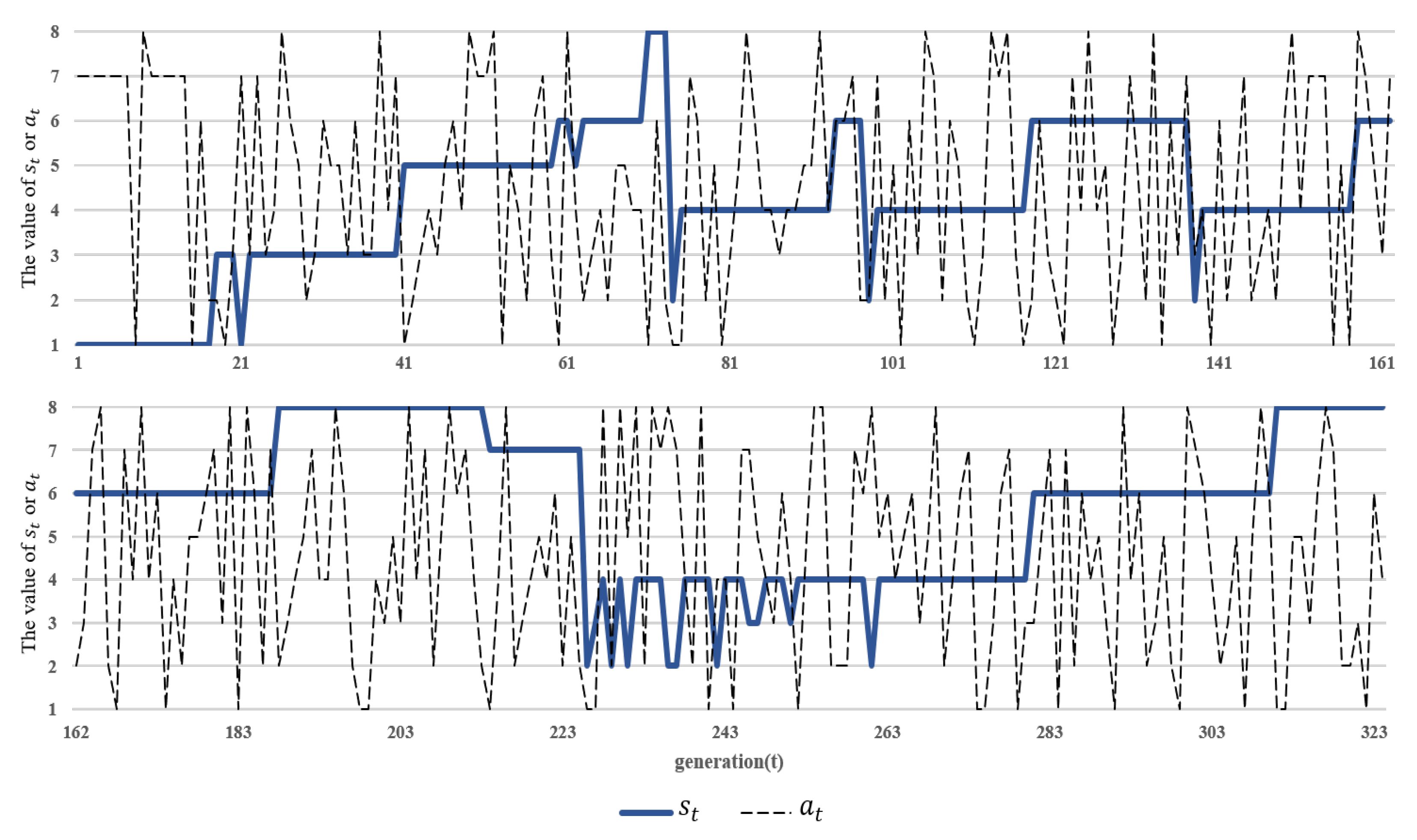
For instance $250\times 5\times 20$, Figure 8 shows the updating processes of state and action. When the stopping condition reaches $t=323$, Figure 8 describes the changes of state and action in the whole process of the Q-learning algorithm. It can be found that population P can keep a state for many generations; for example, the population is in state 6 between generations 162 and 183. Moreover, the action often changes from $a_1$ to $a_8$. An example of the update process of the Q-table is given in Table 4. If $s_t$ = 8, $s_{t+1}$ = 2, $a_t$ = 6, $\alpha$ = 0.1, $\gamma$ = 0.8, $r_{t+1}$ = 1.38 according to Equation (7). As shown in Table 4(a), Q(8, 2) = $-0.879$ before updating, and after the Q-table is updated, $-0.653$ for Q(8, 2) is obtained by Equation (4), which is shown in Table 4(b). The selection of a search operator also exists in a hyper-heuristic, in which a low-level heuristic (LLH) is often selected by using a random method, choice function and tabu search; however, the selection of a hyper-heuristic is often time-consuming. Lin et al. [52] applied a Q-learning algorithm to select an LLH from a set of LLH. Our Q-learning algorithm differs from the work of Lin et al. (1) Fitness proportion is used to depict the state [52], while population evaluation is applied to describe the state in this study. (2) Lin et al. [52] employed a Q-learning algorithm as high-level strategy, which is a part of the hyper-heuristic. The Q-learning algorithm is only adopted to select the search operator and does not substitute any phases of ABC, so in QABC, three phases still exist and are not replaced with Q-learning.

Figure 8. The updated process of state and action.

Table 4. The update process of the Q-table.

				(a)
	$a_1$	$a_2$	$a_3$	$a_4$	$a_5$	$a_6$	$a_7$	$a_8$
$s_1$	0.722	0.697	0.011	0.283	−0.116	0.329	0.245	0.462
$s_2$	−0.175	−0.241	−0.335	−0.218	−0.553	−0.150	−0.256	−0.233
$s_3$	−0.346	−0.297	−0.239	−0.311	−0.361	−0.382	−0.303	−0.272
$s_4$	−0.107	−0.213	−0.113	−0.116	−0.319	−0.118	−0.127	−0.237
$s_5$	−0.111	−0.207	−0.111	−0.112	−0.114	−0.157	0.085	−0.163
$s_6$	−0.560	−0.554	−0.579	−0.459	−0.472	−0.588	−0.468	−0.473
$s_7$	−0.203	−0.209	−0.518	−0.400	−0.746	−0.212	−0.600	−0.385
$s_8$	−0.703	−0.663	−0.858	−0.665	−0.673	−0.879	−0.704	−0.694
				(b)
	$a_1$	$a_2$	$a_3$	$a_4$	$a_5$	$a_6$	$a_7$	$a_8$
$s_1$	0.722	0.697	0.011	0.283	−0.116	0.329	0.245	0.462
$s_2$	−0.175	−0.241	−0.335	−0.218	−0.553	−0.150	−0.256	−0.233
$s_3$	−0.346	−0.297	−0.239	−0.311	−0.361	−0.382	−0.303	−0.272
$s_4$	−0.107	−0.213	−0.113	−0.116	−0.319	−0.118	−0.127	−0.237
$s_5$	−0.111	−0.207	−0.111	−0.112	−0.114	−0.157	0.085	−0.163
$s_6$	−0.560	−0.554	−0.579	−0.459	−0.472	−0.588	−0.468	−0.473
$s_7$	−0.203	−0.209	−0.518	−0.400	−0.746	−0.212	−0.600	−0.385
$s_8$	−0.703	−0.663	−0.858	−0.665	−0.673	−0.653	−0.704	−0.694

4.3. Three Phases of QABC

On each generation of t, two employed bee swarms $E{B}_1$, $E{B}_2$ are used by population division, and the employed bee phase with adaptive migration between them is shown in Algorithm 3, where $mig$ is an integer and $\delta$ is a parameter of migration.

If the condition of migration is met, the worst solution of $E{B}_o,o=1,2$ is replaced with the best solution of $E{B}_{3-o}$; as a result, the worst solutions are deleted, and the best solution of $E{B}_o$ is reproduced.

A simple tournament selection is applied in the onlooker bee phase, and a detailed description is shown in Algorithm 4.

As shown above, when an action $a_{\phi },\phi \le 7$ is selected, according to the Q-learning algorithm, the corresponding search operator, which is composed of a global search, reassignment, inversion and $N{S}_{\phi }$, is used for $E{B}_1$, $E{B}_2$ and $OB$; when action $a_8$ is chosen by the Q-learning algorithm, the search operator from $a_1,a_2,\cdots ,a_7$ is randomly selected for $E{B}_1$, $E{B}_2$, $OB$, respectively.

In general, when $tria{l}_b>Limit$, the corresponding employee bee of $x_b$ will become a scout. In this study, when the condition of the elite solution $x^{*}$ is met, a new scout phase is proposed based on a modified restart strategy [74], which has been proven to be capable of being used to avoid premature convergence. The new scout phase is described in Algorithm 5, where $e{l}^{*}$ is an integer.

In Algorithm 5, when global search, reassignment and inversion are performed on $x_b$, the obtained new solution directly substitutes for $x_b$; that is, greedy selection is not used in the scout phase.

Algorithm 3: Employed bee phase

Input:$E{B}_1,E{B}_2$

1: for $o=1$ to 2 do

2:     for each solution $x\in E{B}_o$ do

3:         execute the chosen search operator of $E{B}_o$ on x

4:     end for

5:     update best solution and worst solution of $E{B}_i$

6: end for

7: if $mig>\delta$ then

8:     for $o=1$ to 2 do

9:         replace the worst solution of $E{B}_o$ with best

10:       solution of $E{B}_{3-o}$

11:     end for

12:     $mig=0$

13: else

14:     $mig=mig+1$

15: end if

Algorithm 4: Onlooker bee phase

1: for each solution $x\in OB$ do

2:     Randomly select $v\in E{B}_1$ and $y\in E{B}_2$

3:     if $fit\left(v\right)<fit\left(y\right)$ then

4:         $x^{{}^{\prime }}=v$

5:     else

6:         $x^{{}^{\prime }}=y$

7:     end if

8:     if $fit\left(x^{{}^{\prime }}\right)<fit\left(x\right)$ then

9:         $x=x^{{}^{\prime }}$

10:     end if

11:     Execute the chosen search operator of $OB$ on x

12: end for

Algorithm 5: Scout phase

Input:$e{l}^{*}$, $Limit$

1: if $e{l}^{*}>Limit$ then

2:     sort all solutions of P in ascending order of $TT$

3:     construct five sets ${\psi }_{\varrho }$, $\varrho \in \{1,2,\cdots ,5\}$

4:     ${\psi }_{\varrho }=\left\{0.2\left(\varrho -1\right)N,0.2\left(\varrho -1\right)N+1,\cdots ,0.2\varrho N\right\}$

5:     for each solution $x_b,b\in {\psi }_2$ do

6:         randomly select a solution $x_{\varrho },\varrho \in {\psi }_1$

7:         execute global search between $x_b$ and $x_{\varrho }$

8:     end for

9:     for each solution $x_b,b\in {\psi }_3$ do

10:         apply reassignment operator on $x_b$

11:     end for

12:     for each solution $x_b,b\in {\psi }_4$ do

13:         perform inversion operator on $x_b$

14:     end for

15:     for each solution $x_b,b\in {\psi }_5$ do

16:         randomly generate a solution

17:     end for

18:     $e{l}^{*}=0$

19: else

20:     $e{l}^{*}=e{l}^{*}+1$

21: end if

22: for each solution $x_b\in P$ do

23:     update $x^{*}$ if $x_b$ is better than $x^{*}$

24: end for

4.4. Algorithm Description

Algorithm 6 gives the detailed steps of QABC, and Figure 9 describes its flow chart, in which t indicates the number of generations, and it also denotes the number of iterations of the Q-learning algorithm.

Algorithm 6: QABC

1: let $mig,e{l}^{*},tria{l}_b,tria{l}^{*}$ be 0, $t=1$

2: Randomly produce an initial population P

3: Initialize Q-table

4: while termination condition is not met do

5:     divide P into $E{B}_1$, $E{B}_2$, and $OB$

6:     select action $a_t$ by Q-learning algorithm

7:     execute employed bee phase by Algorithm 3

8:     perform onlooker bee phase by Algorithm 4

9:     apply scout phase by Algorithm 5

10:     execute reinforcement search on $x^{*}$

11:     update state and Q-table

12:     $t=t+1$

13: end while

Figure 9. The flowchart of QABC.

The reinforcement search of elite solution $x^{*}$ is depicted below. Repeat the following steps $R_2$ times: execute the global search between $x^{*}$ and y ($y\in P$ and $y\ne x^{*}$) and apply reassignment and inversion on $x^{*}$ sequentially, for each operator, when a new solution z is obtained, and $x^{*}$ is updated if z is better than $x^{*}$.

QABC has the following features: (1) The Q-learning algorithm is adopted by using eight states based on the population evaluation, eight actions and a new adaptive action selection strategy. (2) Population P is divided into three swarms $E{B}_1$, $E{B}_2$, $OB$, and the Q-learning algorithm is used to dynamically select a search operator for these swarms. (3) The employed bee phase with adaptive migration and a new scout phase is implemented based on the modified restart method that is used.

In the Q-learning algorithm, eight actions mean that there are eight different search operators, and one of them is dynamically chosen; that is, the evolution of three swarms can be evolved with different operators, and as a result, the exploration ability can be intensified, and the possibility of falling local optima also diminishes greatly. Moreover, a migration and restart can maintain the high diversity of a population; thus, these features may lead to a good performance.

5. Computational Experiments

Extensive experiments were conducted to test the performance of QABC for a distributed three-stage ASP with $DPm\to 1$ layout, factory eligibility and setup times. All experiments were coded in C by using CodeBlocks 16.01 and run on a desktop computer with an Intel i5-10210 CPU (2.10GHz) and 8-GB RAM.

5.1. Test Instances and Comparative Algorithms

A total of 92 instances are applied and depicted by $F\in \left\{2,3,4,5,6\right\}$, $n\in \left\{6,10,20,50,100,200,\right.\left.250,300,500\right\}$ and $m\in \left\{3,5,10,20\right\}$. For each instance denoted as $n\times F\times m$, $p{t}_{ikf},t{t}_{if},a{t}_{if}\in [1,100]$, $sp{t}_{ikf},st{t}_{if},sa{t}_{if}\in [1,20]$, $d_i\in [m\times F\times p{t}_i,n\times p{t}_i]$, where $p{t}_i=({\sum }_{f=1}^F{\sum }_{k=1}^{m}p{t}_{ikf}+sp{t}_{ikf})/F/m$ + $({\sum }_{f=1}^{F}t{t}_{if}+a{t}_{if}+st{t}_{if}+sa{t}_{if})/F$. The elements of ${\mathit{F}}_i$ are randomly selected from $\mathit{F}$, and ${\mathit{F}}_i$ contains at least one factory. The above times and due date are integers and follow a uniform distribution on the above intervals.

As stated above, distributed ASP with factory eligibility is not considered, and there are no existing comparative algorithms.

For the distributed heterogeneous flowshop scheduling problem, Chen et al. [75] presented a probability model-based memetic algorithm (PMMA) with search operators and a local intensification operator, Li et al. [64] proposed a discrete artificial bee colony (DABC) with neighborhood search operators, a new acceleration method and a population update method, and Meng and Pan [65] designed an enhanced artificial bee colony (NEABC) by using a collaboration mechanism and restart strategy.

PMMA [75], DABC [64] and NEABC [65] have been successfully applied to solve the above distributed flowshop scheduling; moreover, these algorithms can be directly used to solve distributed three-stage ASP with factory eligibility after transportation and assembly are added into decoding process, and thus they are chosen as comparative algorithms.

Two variants named ABC1 and ABC2 are constructed. When the Q-learning algorithm is removed from QABC, ABC1 is obtained. When population division, migration, restart, and reinforcement search are removed from ABC1, and a scout phase is implemented as in Section 3.1, ABC2 is produced. When the Q-learning algorithm is removed, the search operator of P is fixed. We tested seven search operators, and two variants with $a_1$ is better than these algorithms with other operators.

5.2. Parameter Settings

In this study, a stopping condition is defined by CPU time. We found through experiments that QABC converges fully on all instances when $0.5\times n$ seconds is reached; moreover, all comparative algorithms, ABC1 and ABC2, also converge fully when this CPU time is reached, and so we set $0.5\times n$ seconds as the stopping condition of all algorithms.

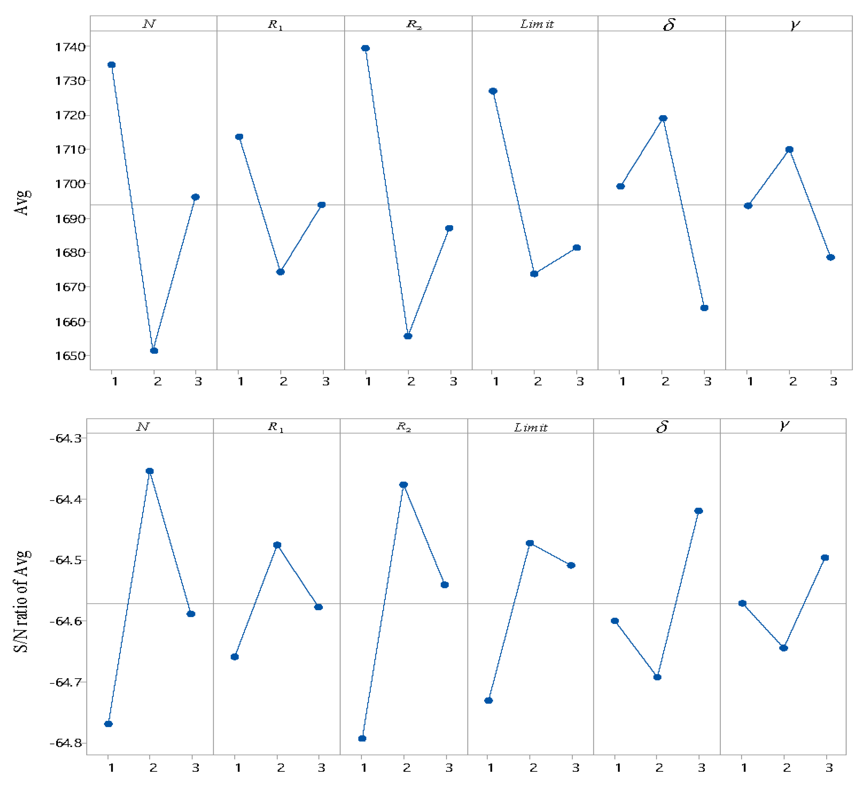
With respect to the parameters of the Q-learning algorithm, we directly use the initial $\epsilon$ of 0.9 and learning rate $\alpha =0.1$, according to Wang et al. [76]. The following parameters of QABC, which are N, $R_1$, $R_2$, $Limit$, $\delta$ and discount rate $\gamma$ are tested according to the Taguchi method [77] on instance $250\times 5\times 10$. The levels of each parameter are shown in Table 5. The results of $Avg$ and the S/N ratio are given in Figure 10, where $Avg$ is the average value of 10 elite solutions in 10 runs, $Avg={\sum }_{g=1}^{10}elit{e}_g/10$, $elit{e}_g$ represents the elite solution for the gth run, and the S/N ratio is defined as $-10{log}_{10}\left(Av{g}^2\right)$.

Table 5. Levels of the parameters.

Parameters	Factor Level
	1	2	3
N	120	150	180
$R_1$	20	40	50
$R_2$	30	50	70
$Limit$	100	150	200
$\delta$	50	75	100
$\gamma$	0.4	0.6	0.8

Figure 10. Mean $Avg$ and mean S/N ratio.

As shown in Figure 10, when the levels of N, $R_1$, $R_2$, $Limit$, $\delta$, and $\gamma$ are 2, 2, 2, 2, 3, 3, QABC produces a smaller average $Avg$ and a bigger S/N ratio than QABC with other combinations of levels, and so the suggested settings are $N=150$, $R_1=40$, $R_1=50$, $Limit=150$, $\delta =100$ and $\gamma =0.8$.

Parameters of ABC1 and ABC2 are directly selected from QABC. Except for the stopping condition, the other parameters of PMMA, DABC, and NEABC are chosen from [64,65,75]. We also found that these settings of comparative algorithms can result in a better performance than other settings.

5.3. Results and Analyses

QABC is compared with ABC1, ABC2, PMMA, DABC and NEABC. Each algorithm randomly runs 10 times on each instance. Table 6, Table 7 and Table 8 show the computational results of QABC and its comparative algorithms, where $Min$ indicates the smallest total tardiness in 10 runs, $Min=\underset{g=1,2,\cdots ,10}{min}elit{e}_g$, and $STD$ is the standard deviation for 10 elite solutions in 10 runs, $STD=\sqrt{{\sum }_{g=1}^{10}{(elit{e}_g-Avg)}^2/10}$. QA, A1, A2, PM, DA and NE denote QABC, ABC1, ABC2, PMMA, DABC and NEABC for simplicity, respectively. 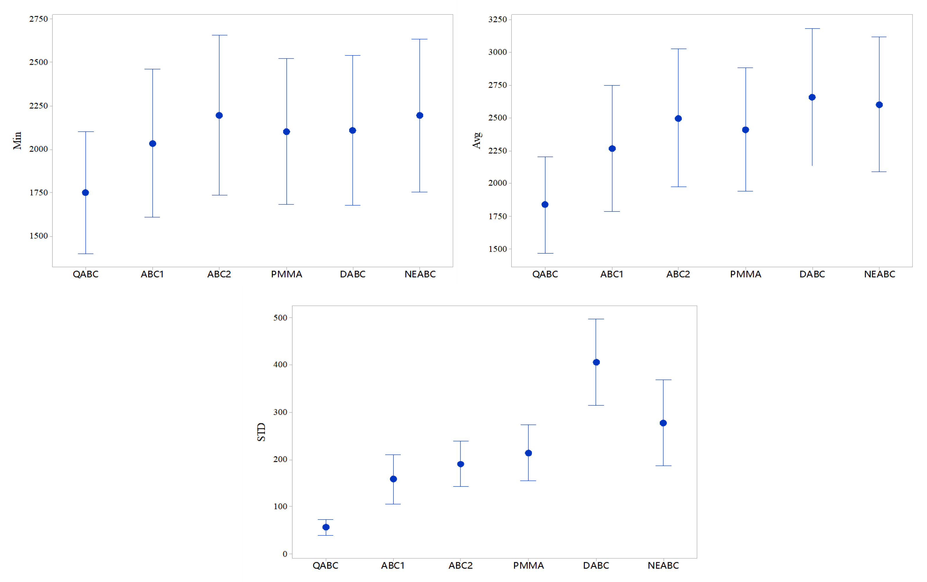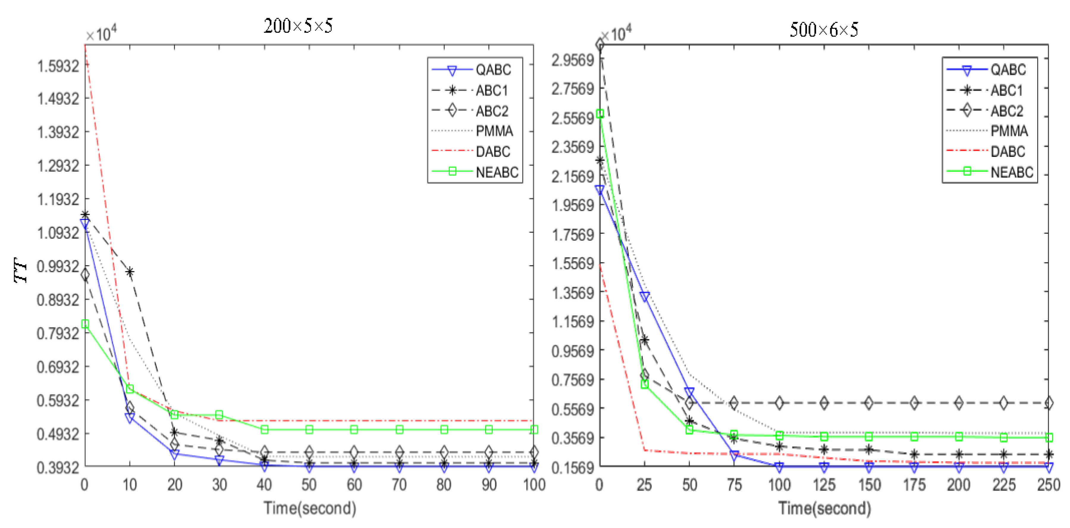Figure 11 displays the mean plot with a 95% confidence interval of all algorithms, and Figure 12 describes convergence curves for instances $200\times 5\times 5$ and $500\times 6\times 5$. Table 9 shows the results of pair-sample t-test, in which t-test (A, B) means that a paired t-test is conducted to judge whether algorithm A gives a better sample mean than B. If a significance level is 0.05, there is a significant difference between A and B in the statistical sense if the p-value is less than 0.05.

Table 6. Computational results of $Min$ by six algorithms.

$\mathit{n}\times \mathit{F}\times \mathit{m}$	QA	A1	A2	PM	DA	NE	$\mathit{n}\times \mathit{F}\times \mathit{m}$	QA	A1	A2	PM	DA	NE
$6\times 2\times 3$	827	827	827	827	827	827	$100\times 4\times 20$	2753	3097	2974	3068	3580	3244
$6\times 2\times 5$	568	568	568	568	568	568	$100\times 5\times 5$	1964	1964	2105	2003	2286	2251
$10\times 2\times 3$	576	576	576	576	592	576	$100\times 5\times 10$	1179	1179	1179	1179	1252	1280
$10\times 2\times 5$	808	808	808	808	808	808	$100\times 5\times 20$	1468	1675	1849	1553	2272	2157
$6\times 3\times 3$	66	66	66	66	66	157	$100\times 6\times 5$	1088	1088	1088	1088	1211	1106
$6\times 3\times 5$	92	92	92	92	92	232	$100\times 6\times 10$	1008	1018	1103	1052	1153	1265
$10\times 3\times 3$	73	73	73	73	73	90	$100\times 6\times 20$	913	913	957	913	1046	1006
$10\times 3\times 5$	112	112	112	112	112	237	$200\times 2\times 5$	140	251	729	242	344	209
$20\times 2\times 5$	1973	1973	1973	1973	2066	1973	$200\times 2\times 10$	718	4677	1419	788	502	1162
$20\times 2\times 10$	1459	1459	1459	1459	1470	1477	$200\times 2\times 20$	4516	9205	8122	4855	8060	4974
$20\times 2\times 20$	915	915	922	915	971	915	$200\times 3\times 5$	429	475	451	495	507	891
$20\times 3\times 5$	1741	1741	1741	1741	1762	1741	$200\times 3\times 10$	2608	3108	3315	3167	3057	3672
$20\times 3\times 10$	111	111	111	111	126	154	$200\times 3\times 20$	509	509	525	617	509	509
$20\times 3\times 20$	768	768	768	768	780	768	$200\times 4\times 5$	1630	1638	1808	2016	2075	2072
$20\times 4\times 5$	1228	1228	1228	1228	1361	1239	$200\times 4\times 10$	576	626	635	690	785	723
$20\times 4\times 10$	680	680	680	680	724	753	$200\times 4\times 20$	879	988	1075	1098	1068	1309
$20\times 4\times 20$	1354	1354	1359	1354	1410	1402	$200\times 5\times 5$	3845	4135	4304	4225	4181	4867
$20\times 5\times 5$	684	684	684	684	757	779	$200\times 5\times 10$	886	959	1012	924	1098	1044
$20\times 5\times 10$	1228	1228	1228	1820	1866	1341	$200\times 5\times 20$	5928	6516	6344	6384	7097	6605
$20\times 5\times 20$	950	950	950	950	984	1071	$200\times 6\times 5$	3321	3429	3436	3537	3718	3934
$20\times 6\times 5$	321	321	321	321	321	798	$200\times 6\times 10$	911	911	911	927	1002	979
$20\times 6\times 10$	1217	1217	1217	1217	1293	1368	$200\times 6\times 20$	694	716	745	695	780	838
$20\times 6\times 20$	949	949	949	956	949	1212	$250\times 3\times 5$	5275	7604	9537	7427	6089	7459
$50\times 2\times 5$	6382	6501	6531	6550	6914	6524	$250\times 3\times 10$	2723	3384	5204	3413	3256	3640
$50\times 2\times 10$	5781	5781	5821	5781	5949	5958	$250\times 3\times 20$	769	1722	5390	1428	955	1721
$50\times 2\times 20$	2617	2732	2757	2780	2922	3150	$250\times 4\times 5$	1106	1218	1247	1349	1267	1477
$50\times 3\times 5$	733	733	746	733	1240	733	$250\times 4\times 10$	4523	5462	5269	6244	5995	5457
$50\times 3\times 10$	3883	3943	4004	3967	4466	4265	$250\times 4\times 20$	2423	3015	3413	2984	4287	2907
$50\times 3\times 20$	5118	5296	5367	5318	5531	5626	$250\times 5\times 5$	5952	6706	6853	6975	6819	8730
$50\times 4\times 5$	934	934	959	943	1136	955	$250\times 5\times 10$	1656	2099	2270	2338	2589	2577
$50\times 4\times 10$	1044	1048	1151	1051	1274	1075	$250\times 5\times 20$	280	340	352	418	340	393
$50\times 4\times 20$	541	541	561	541	618	581	$250\times 6\times 5$	7367	7918	9303	8402	8014	9628
$50\times 5\times 5$	570	570	573	570	663	570	$250\times 6\times 10$	2028	2505	2447	2308	2398	2408
$50\times 5\times 10$	591	591	592	591	666	621	$250\times 6\times 20$	3939	4518	5354	4585	4272	5169
$50\times 5\times 20$	840	840	840	840	867	856	$300\times 5\times 5$	644	817	1596	1330	712	1356
$50\times 6\times 5$	552	552	562	552	592	552	$300\times 5\times 10$	2733	3141	4122	4150	3891	4647
$50\times 6\times 10$	102	102	102	102	110	102	$300\times 5\times 20$	162	213	334	672	261	587
$50\times 6\times 20$	675	675	762	696	813	851	$300\times 6\times 5$	5682	6509	7374	7141	6091	7840
$100\times 2\times 5$	4205	4457	4419	4387	4937	5064	$300\times 6\times 10$	2205	2584	3181	3639	2314	3291
$100\times 2\times 10$	1250	1421	1491	1284	1427	1364	$300\times 6\times 20$	3094	3883	4542	5175	3750	4703
$100\times 2\times 20$	3221	3679	4316	3306	6075	3547	$500\times 5\times 5$	720	738	738	1396	730	920
$100\times 3\times 5$	673	677	676	673	1138	691	$500\times 5\times 10$	1485	1642	1617	3235	1972	2120
$100\times 3\times 10$	3687	4521	4631	3944	6109	4505	$500\times 5\times 20$	117	121	140	484	166	294
$100\times 3\times 20$	737	737	576	750	806	862	$500\times 6\times 5$	1098	1883	3966	2008	924	2257
$100\times 4\times 5$	826	842	885	836	915	872	$500\times 6\times 10$	1039	1154	1230	1883	1161	1643
$100\times 4\times 10$	903	928	1009	933	1221	1253	$500\times 6\times 20$	1542	2296	2499	6505	1969	3679

Table 7. Computational results of $Avg$ by six algorithms.

$\mathit{n}\times \mathit{F}\times \mathit{m}$	QA	A1	A2	PM	DA	NE	$\mathit{n}\times \mathit{F}\times \mathit{m}$	QA	A1	A2	PM	DA	NE
6 × 2 × 3	827.0	827.0	827.0	827.0	827.0	857.0	100 × 4 × 20	2883.9	3266.3	3393.1	3278.2	4108.8	3562.2
6 × 2 × 5	568.0	568.0	568.0	568.0	568.0	568.0	100 × 5 × 5	1989.1	1993.5	2343.0	2110.1	2681.4	2451.4
10 × 2 × 3	576.0	576.0	576.0	576.0	592.0	576.0	100 × 5 × 10	1179.0	1182.3	1246.1	1197.6	1394.7	1353.8
10 × 2 × 5	808.0	808.0	808.0	808.0	808.0	818.8	100 × 5 × 20	1560.0	1970.0	2047.4	1677.0	2627.2	2408.2
6 × 3 × 3	66.0	66.0	66.0	66.0	66.0	157.0	100 × 6 × 5	1088.0	1097.6	1120.8	1098.5	1312.9	1194.7
6 × 3 × 5	92.0	92.0	92.0	92.0	92.0	232.0	100 × 6 × 10	1027.3	1114.2	1254.6	1119.6	1444.2	1390.1
10 × 3 × 3	73.0	73.0	73.0	74.0	74.1	90.0	100 × 6 × 20	913.0	916.3	1067.5	989.8	1336.9	1136.8
10 × 3 × 5	112.0	112.0	112.0	112.0	112.0	252.5	200 × 2 × 5	229.9	617.5	1170.2	478.5	788.2	621.1
20 × 2 × 5	1973.0	1973.0	1994.9	2006.9	2119.2	2022.2	200 × 2 × 10	1323.1	7161.0	2500.5	1332.7	1122.1	1956.3
20 × 2 × 10	1459.0	1459.0	1476.9	1459.3	1558.3	1747.5	200 × 2 × 20	4894.6	10,303.7	9547.8	5896.1	9525.1	11,185.9
20 × 2 × 20	915.0	917.1	948.0	927.4	1066.7	1125.0	200 × 3 × 5	466.7	595.6	754.4	908.8	1179.8	1297.8
20 × 3 × 5	1741.0	1741.0	1756.7	1749.4	1782.4	1759.8	200 × 3 × 10	2781.9	3396.3	3594.0	3779.4	4182.0	4171.5
20 × 3 × 10	111.0	111.0	121.0	122.5	190.8	283.7	200 × 3 × 20	515.4	550.2	699.5	762.2	1180.4	780.2
20 × 3 × 20	768.0	768.0	775.2	770.8	822.7	837.1	200 × 4 × 5	1691.9	1822.6	2011.9	2120.5	2885.7	2294.5
20 × 4 × 5	1228.0	1229.6	1253.8	1342.3	1438.4	1517.2	200 × 4 × 10	582.4	726.6	801.7	773.8	989.8	924.8
20 × 4 × 10	680.0	682.3	716.1	707.8	826.7	810.2	200 × 4 × 20	940.6	1163.5	1144.2	1398.7	1415.8	1761.5
20 × 4 × 20	1354.0	1356.4	1374.0	1378.0	1503.0	1577.5	200 × 5 × 5	4020.5	4451.3	4718.9	4423.4	4987.8	5332.8
20 × 5 × 5	684.0	684.0	712.4	731.1	832.1	1087.5	200 × 5 × 10	943.4	1100.1	1173.7	1042.2	1472.0	1343.5
20 × 5 × 10	1228.0	1230.6	1248.6	1836.5	1956.1	1527.4	200 × 5 × 20	6063.3	6806.9	6574.8	6766.8	8226.4	6850.5
20 × 5 × 20	950.0	950.0	1002.3	998.4	1124.6	1238.0	200 × 6 × 5	3379.4	3630.1	3697.0	3760.3	4100.8	4166.8
20 × 6 × 5	321.0	321.0	322.9	323.9	352.0	921.4	200 × 6 × 10	911.0	945.3	983.1	965.8	1079.0	1039.6
20 × 6 × 10	1217.0	1217.0	1247.5	1270.3	1350.2	1584.2	200 × 6 × 20	694.0	781.1	874.5	791.2	997.0	982.3
20 × 6 × 20	949.0	949.0	963.9	977.9	1037.4	1321.9	250 × 3 × 5	6102.7	8676.4	10,756.0	8596.2	8927.3	9505.3
50 × 2 × 5	6429.7	6588.7	6952.9	6683.9	7610.3	7466.0	250 × 3 × 10	2868.1	4335.8	6686.2	4983.9	5523.4	4614.3
50 × 2 × 10	5807.2	5826.7	6050.0	5883.7	6316.6	6233.1	250 × 3 × 20	1011.5	3123.9	7648.0	2737.6	2319.9	2871.2
50 × 2 × 20	2686.2	2855.6	2984.5	2924.3	3522.9	3390.1	250 × 4 × 5	1181.9	1449.6	1410.9	1755.4	2008.3	1654.7
50 × 3 × 5	733.0	733.0	803.9	757.0	1506.8	886.5	250 × 4 × 10	4812.8	6459.4	6521.1	6892.6	8250.8	6260.2
50 × 3 × 10	3953.2	3996.5	4151.5	4052.1	5196.0	4543.2	250 × 4 × 20	2530.1	3466.9	4405.0	4082.0	6169.1	3463.3
50 × 3 × 20	5195.2	5368.4	5554.3	5448.7	5840.8	6284.7	250 × 5 × 5	6286.4	7597.5	7951.9	7856.9	8185.4	9400.7
50 × 4 × 5	934.6	937.8	1016.3	1047.2	1377.8	1041.3	250 × 5 × 10	1837.5	2481.4	2449.6	2590.9	3776.1	3206.7
50 × 4 × 10	1044.8	1087.7	1250.5	1153.5	1447.9	1420.6	250 × 5 × 20	297.1	412.8	437.3	571.4	579.8	571.6
50 × 4 × 20	546.9	556.3	609.4	600.5	714.9	737.5	250 × 6 × 5	7883.2	8967.5	10,104.2	9249.0	8856.2	9934.1
50 × 5 × 5	572.7	585.8	663.8	597.7	774.3	706.9	250 × 6 × 10	2131.0	2659.5	2593.0	2848.1	3428.7	2789.1
50 × 5 × 10	591.4	597.4	646.0	609.2	780.6	712.3	250 × 6 × 20	4125.0	5173.7	6546.1	6109.5	5405.4	5694.0
50 × 5 × 20	840.0	840.0	895.6	844.2	1055.6	965.7	300 × 5 × 5	812.0	1184.3	2051.2	1742.4	1071.6	2107.3
50 × 6 × 5	552.0	555.7	600.4	570.7	764.3	608.4	300 × 5 × 10	2992.9	3683.0	4604.2	5320.9	4739.7	5623.3
50 × 6 × 10	102.0	102.0	113.7	108.4	192.2	167.8	300 × 5 × 20	215.4	421.8	433.5	807.1	491.8	824.4
50 × 6 × 20	704.9	733.0	885.4	783.8	1027.9	975.3	300 × 6 × 5	6159.2	7175.1	7883.8	8126.9	6898.7	8684.9
100 × 2 × 5	4379.3	4867.7	5445.6	4763.3	7439.9	5717.6	300 × 6 × 10	2390.9	3114.0	3429.9	4060.5	3559.3	3856.0
100 × 2 × 10	1323.8	1535.0	1909.0	1326.0	2517.1	1979.2	300 × 6 × 20	3437.0	4312.8	5199.9	5807.9	4993.6	5342.2
100 × 2 × 20	3352.8	4482.3	5221.7	3449.9	7557.2	3973.4	500 × 5 × 5	727.1	824.4	915.9	2684.7	1023.1	1389.4
100 × 3 × 5	673.4	699.9	760.5	692.1	1480.7	772.3	500 × 5 × 10	1538.5	1910.8	1806.6	4082.8	2648.9	2362.5
100 × 3 × 10	3886.9	4755.2	5054.5	4505.6	8002.7	5265.6	500 × 5 × 20	119.8	154.7	159.3	1499.4	212.2	632.8
100 × 3 × 20	737.0	766.1	638.0	813.0	1373.7	1044.6	500 × 6 × 5	1344.5	2625.9	5230.5	4003.6	1651.6	3380.1
100 × 4 × 5	842.7	875.2	955.0	867.8	1265.4	1183.3	500 × 6 × 10	1091.1	1448.6	1433.9	2430.0	1984.4	2006.9
100 × 4 × 10	909.6	1076.1	1223.3	1050.7	1707.3	1508.5	500 × 6 × 20	1763.4	2545.8	3108.4	7247.6	2578.6	4670.5

Table 8. Computational results of $STD$ by six algorithms.

$\mathit{n}\times \mathit{F}\times \mathit{m}$	QA	A1	A2	PM	DA	NE	$\mathit{n}\times \mathit{F}\times \mathit{m}$	QA	A1	A2	PM	DA	NE
6 × 2 × 3	0.0	0.0	0.0	0.0	0.0	24.5	100 × 4 × 20	87.4	125.5	269.8	109.5	400.0	253.4
6 × 2 × 5	0.0	0.0	0.0	0.0	0.0	0.0	100 × 5 × 5	25.4	40.5	248.9	83.8	389.4	138.3
10 × 2 × 3	0.0	0.0	0.0	0.0	0.0	0.0	100 × 5 × 10	0.0	6.5	74.7	24.4	74.1	61.6
10 × 2 × 5	0.0	0.0	0.0	0.0	0.0	20.6	100 × 5 × 20	68.2	175.9	172.4	94.0	386.7	232.6
6 × 3 × 3	0.0	0.0	0.0	0.0	0.0	0.0	100 × 6 × 5	0.0	4.8	26.8	7.3	101.6	64.0
6 × 3 × 5	0.0	0.0	0.0	0.0	0.0	0.0	100 × 6 × 10	23.6	72.9	82.0	74.2	232.3	157.2
10 × 3 × 3	0.0	0.0	0.0	2.0	2.0	0.0	100 × 6 × 20	0.0	8.0	65.2	45.9	227.7	107.0
10 × 3 × 5	0.0	0.0	0.0	0.0	0.0	14.6	200 × 2 × 5	75.2	240.7	408.9	219.4	307.7	413.5
20 × 2 × 5	0.0	0.0	23.1	52.1	29.0	58.2	200 × 2 × 10	318.6	1478.1	1137.2	348.3	924.0	488.7
20 × 2 × 10	0.0	0.0	23.0	0.9	85.5	160.5	200 × 2 × 20	222.6	767.6	719.0	777.7	1580.5	3866.4
20 × 2 × 20	0.0	3.2	19.0	10.3	54.9	108.8	200 × 3 × 5	22.7	101.3	183.6	364.0	555.2	363.4
20 × 3 × 5	0.0	0.0	10.5	6.7	34.3	8.9	200 × 3 × 10	131.2	177.9	206.2	456.8	782.1	315.2
20 × 3 × 10	0.0	0.0	12.3	8.0	45.8	63.4	200 × 3 × 20	19.2	34.5	136.5	94.8	475.6	168.9
20 × 3 × 20	0.0	0.0	9.1	5.7	16.8	66.7	200 × 4 × 5	54.5	83.1	114.4	99.1	735.9	146.1
20 × 4 × 5	0.0	4.8	21.6	45.0	57.4	147.6	200 × 4 × 10	12.6	72.4	109.7	47.3	185.5	154.1
20 × 4 × 10	0.0	6.9	27.5	28.0	79.9	71.4	200 × 4 × 20	47.6	130.0	71.7	211.0	235.2	313.6
20 × 4 × 20	0.0	7.2	7.4	20.4	68.1	160.1	200 × 5 × 5	76.5	222.4	337.3	159.5	528.0	278.9
20 × 5 × 5	0.0	0.0	32.9	47.4	60.9	269.7	200 × 5 × 10	41.4	113.6	105.8	78.7	244.5	185.8
20 × 5 × 10	0.0	5.2	20.2	19.3	78.5	113.8	200 × 5 × 20	68.0	233.9	161.8	164.4	773.4	177.9
20 × 5 × 20	0.0	0.0	50.6	41.4	83.4	211.0	200 × 6 × 5	51.1	134.4	203.7	134.4	377.8	196.2
20 × 6 × 5	0.0	0.0	5.7	6.1	29.2	110.5	200 × 6 × 10	0.0	30.5	35.8	30.0	67.8	69.6
20 × 6 × 10	0.0	0.0	25.8	31.0	44.5	110.8	200 × 6 × 20	0.0	62.1	79.9	84.7	165.5	84.8
20 × 6 × 20	0.0	0.0	19.7	14.6	55.0	101.9	250 × 3 × 5	360.9	822.7	788.0	1280.3	1986.1	1513.4
50 × 2 × 5	41.1	73.8	218.0	89.9	443.4	557.0	250 × 3 × 10	143.6	598.7	645.9	913.7	1567.2	486.9
50 × 2 × 10	41.5	44.2	176.7	89.9	364.1	220.1	250 × 3 × 20	159.5	900.1	880.8	837.4	1070.6	832.2
50 × 2 × 20	66.1	63.2	174.7	106.3	434.3	237.6	250 × 4 × 5	45.6	132.8	111.3	256.0	490.7	158.2
50 × 3 × 5	0.0	0.0	52.8	49.3	170.6	127.5	250 × 4 × 10	215.0	542.4	610.8	370.7	1650.3	447.6
50 × 3 × 10	27.7	31.7	97.7	95.5	431.7	165.3	250 × 4 × 20	70.5	306.7	506.9	524.3	1126.1	436.9
50 × 3 × 20	55.2	66.8	136.5	120.3	403.6	420.5	250 × 5 × 5	279.2	533.1	561.0	528.0	1367.1	374.7
50 × 4 × 5	1.8	2.7	36.6	87.6	131.2	53.7	250 × 5 × 10	79.5	261.9	126.0	228.2	577.8	379.7
50 × 4 × 10	1.6	27.2	88.6	52.8	111.8	564.7	250 × 5 × 20	24.5	48.4	64.5	149.4	147.4	151.1
50 × 4 × 20	6.1	15.4	30.0	30.8	93.6	100.4	250 × 6 × 5	316.7	804.8	475.2	639.2	754.1	276.4
50 × 5 × 5	5.2	20.9	57.8	28.3	51.2	85.4	250 × 6 × 10	49.9	144.5	119.0	246.5	656.5	252.5
50 × 5 × 10	0.7	11.5	42.8	21.0	114.8	74.3	250 × 6 × 20	154.1	431.4	591.4	989.7	742.5	232.1
50 × 5 × 20	0.0	0.0	60.3	7.7	124.8	69.4	300 × 5 × 5	111.9	266.0	381.1	360.2	164.2	383.7
50 × 6 × 5	0.0	4.4	41.7	17.8	118.5	66.5	300 × 5 × 10	179.6	303.0	293.7	586.7	570.1	584.0
50 × 6 × 10	0.0	0.0	12.8	8.5	56.2	60.0	300 × 5 × 20	35.8	121.8	67.8	76.3	184.8	143.2
50 × 6 × 20	31.7	60.3	87.3	45.1	123.9	72.7	300 × 6 × 5	251.3	436.7	390.7	672.2	581.5	445.9
100 × 2 × 5	141.0	193.5	666.2	322.0	1503.3	648.7	300 × 6 × 10	91.3	333.0	136.4	349.3	948.2	273.4
100 × 2 × 10	40.3	73.0	358.9	29.1	994.4	542.5	300 × 6 × 20	215.3	518.7	307.2	464.7	797.5	415.7
100 × 2 × 20	62.6	402.7	521.6	85.7	1132.7	370.3	500 × 5 × 5	4.2	72.0	129.1	754.3	397.6	229.8
100 × 3 × 5	1.2	36.6	66.9	35.9	183.5	62.3	500 × 5 × 10	31.6	147.8	224.0	762.2	368.7	185.0
100 × 3 × 10	113.8	167.2	512.7	436.3	1079.3	490.0	500 × 5 × 20	4.6	20.0	12.8	742.0	41.7	471.6
100 × 3 × 20	0.0	27.7	109.1	51.0	330.1	145.7	500 × 6 × 5	192.9	635.0	634.1	1014.8	393.3	513.9
100 × 4 × 5	13.9	19.9	49.8	33.2	341.1	172.6	500 × 6 × 10	44.6	206.3	103.4	246.2	527.6	335.5
100 × 4 × 10	4.7	111.8	150.5	95.0	378.2	155.7	500 × 6 × 20	119.0	195.2	389.1	752.8	592.2	538.5

Figure 11. Mean plot with 95% confidence interval for all algorithms.

Figure 12. Convergence curves of two instances.

Table 9. Results of paired sample t-test.

t-Test	p_Value($\mathit{Min}$)	p_Value($\mathit{Avg}$)	p_Value($\mathit{STD}$)
t-test (QABC, ABC1)	0.0001	0.0000	0.0000
t-test (QABC, ABC2)	0.0000	0.0000	0.0000
t-test (QABC, PMMA)	0.0000	0.0000	0.0000
t-test (QABC, DABC)	0.0000	0.0000	0.0000
t-test (QABC, NEABC)	0.0000	0.0000	0.0000

As shown in Table 6, Table 7 and Table 8, QABC significantly performs better than ABC1 in most of the instances. The $Min$ of QABC is smaller than that of ABC1 by at least 10% in 31 instances, $Avg$ of QABC is less than that of ABC1 by at least 200 in more than 35 instances and $STD$ of QABC is smaller than that of ABC1 in nearly all instances. Table 9 shows that there are notable performance differences between QABC and ABC1 in a statistical sense. Figure 11 depicts the notable differences between the $STD$ of the two algorithms, and Figure 12 reveals that QABC significantly converges better than ABC1.

It can be found from Table 6 that ABC1 produces better $Min$ than ABC2 in 54 of 92 instances. As shown in Table 7, $Avg$ of ABC1 is less than or equal to that of ABC2 in 84 of 92 instances. Table 8 shows that ABC2 performs better than ABC1 on $STD$ in 64 instances. Figure 12 and Table 9 also reveal that ABC1 performed better than ABC2.

Although some new parameters such as $\delta$ and $\gamma$ are added because of the inclusion of new strategies such as Q-learning and migration, the above analyses on ABC, ABC1 and ABC2 demonstrate that the Q-learning algorithm, migration and new scout phase, etc., have really positive impacts on the performance of QABC, and thus, these new strategies are effective and reasonable.

As shown in Table 6, Table 7 and Table 8, QABC and PMMA converge to the same best solution for most of the instances with $n<100$, QABC does not generate worse $Min$ than PMMA in any instances with $n\ge 100$; moreover, QABC produces $Avg$ and $STD$ smaller than or the same as PMMA in almost all instances. QABC performs better than PMMA. The statistical results in Table 9 also reveal the above conclusion can be obtained. Figure 11 and Figure 12 show the performance difference between the two algorithms regarding $STD$ and $Min$, respectively.

When QABC is compared with DABC, it can be seen from Table 6, Table 7 and Table 8 that QABC has smaller $Min$ than DABC in 80 instances, generates smaller $Avg$ than DABC in 85 instances and obtains smaller $STD$ than DABC in 85 instances; moreover, performance differences between QABC and DABC increase with an increase in $n\times F\times m$. The convergent curves in Figure 12 and results in Table 9 can also demonstrate the performance difference in $Min$ between QABC and DABC, the performance differences in $Avg$ also can be validated by the statistical results in Table 9, and Figure 11 and Table 9 show that QABC significantly outperforms DABC in $STD$.

It can be concluded from Table 6, Table 7 and Table 8 that QABC performs significantly better than NEABC. QABC produces smaller $Min$ than NEABC by at least 20% in about 39 instances, also generates better $Avg$ than NEABC by at least 20% in more than 58 instances and obtains better $STD$ than or the same $STD$ as NEABC on nearly all instances. QABC performs notably better than NEABC, and the same conclusion can be found in Table 9. Figure 11 shows the significant difference in $STD$, and Figure 12 demonstrates the notable convergence advantage of QABC.

As stated above, the inclusion of the Q-learning algorithm, the migration between two employed bee swarms and modified restart strategy in the scout phase really improve the performance of QABC. The Q-learning algorithm results in the dynamical adjustment of search operators in the employed bee phase and onlooker bee phase. As a result, the search operator is not fixed and varied dynamically, and the exploration ability can be improved. Migration leads to the full use of the best solutions of $E{B}_1$ and $E{B}_2$, and the restart strategy makes the population evolve with higher diversity. These features can lead to better search efficiency. Based on the above analyses, it can be concluded that QABC can effectively solve the distributed three-stage ASP with factory eligibility and setup times.

6. Conclusions

DASP has attracted some attention in recent years; however, a distributed three-stage ASP with various actual production constraints is seldom investigated. In this study, a distributed three-stage ASP with a $DPm\to 1$ layout, factory eligibility and setup times is considered. An effective QABC algorithm is developed to minimize total tardiness. In QABC, a Q-learning algorithm is implemented with eight states, eight actions, a new reward and an effective adaptive $ϵ$-greedy action selection and is adopted to dynamically decide the search operator for $E{B}_1$, $E{B}_2$ and $OB$, obtained initially by population division. Adaptive migration between $E{B}_1$ and $E{B}_2$ and a modified restart strategy are executed in the employed bee phase and scout phase, respectively. A number of experiments are conducted, and the experimental results validate that QABC has reasonable and effective strategies and very competitive performances on the considered problem.

The distributed three-stage ASP is our main topic in the near future. We will focus on distributed three-stage ASP with other constraints such as fuzzy processing time and stochastic breakdown. We are also interested in other distributed scheduling problems, such as the distributed flexible job shop scheduling and distributed hybrid flow shop scheduling. Swarm intelligence optimizations and RL are also the focus of our attention, and we will try to carry out more effective combination modes and innovative strategies. We will also pay attention to the multi-objective optimization problem in distributed production networks.