PIV Measurement and Proper Orthogonal Decomposition Analysis of Annular Gap Flow of a Hydraulic Machine

Abstract

The fluid stress or flow-induced vibration of annular gap flow always has some influence on the stable working conditions of a hydraulic machine. A time-averaged analysis of flow may not have to explicitly acknowledge these factors. Accordingly, a finite-axial-length annular gap was measured via particle image velocimetry (PIV), with inner boundary motion and a stable outer boundary. As a statistic result regarding the fluid stress, the Reynolds stresses soared in the first region, were sustained in the middle region, but decreased at last. The flow had a higher convective transportation intensity in the radial direction than in other directions. Flow diagnostics were also performed by proper orthogonal decomposition (POD). As a result, the coherent structures were found. Then, the power spectrum density (PSD) functions were also calculated for finding the flow-induced vibration characteristics; the functions had high amplitude in the low-frequency domain and low amplitude in the high-frequency domain, with an order of magnitude between the two amplitudes of 10⁻¹ to 10⁻². In addition, the frequency was higher at a smaller gap width in the middle-frequency domain, but the condition was the opposite in the high-frequency domain. In conclusion, the fluid stresses were changeable and uneven along the flow direction, and flow-induced vibration obviously existed. Remarkably, the turbulence characteristics of the annular gap flow were not “laminar approximating,” while the diameter ratio of the gap was 0.6 to 0.8.

1. Introduction

In various types of hydraulic machinery, as these hydraulic machines work, different types of flow are produced between their gap boundaries [1,2]. Traditional gap flow theory is based on the one-dimensional flow theory of hydraulics, where some two-dimensional flow or three-dimensional flow, normally treated as laminar flow, is moderately amended and used to calculate the averaged velocity of gap flow, giving a constant flow view. However, “laminar approximating” is for a gap with an extremely minor width; as for a slightly larger gap width, some studies [3,4,5] have demonstrated that there are differences in the three main aspects between the laminar approximating and turbulence pattern of gap flow.

The first aspect is the flow structure. For the laminar approximating pattern, the flow can be regarded as parallel flow: the streamlines are parallel with each other, and there is no obvious flow structure. However, earlier evidence indicated that there are no straight parallel streamlines in annular gap flow. There was a backwash vortex attached on the inner boundary near the inlet of annular gap flow in a hydraulic pipeline transportation system (Liu et al. [6]). The second aspect is the fluid stresses. The flow structures exist in different locations of the annular gap flow, and the fluid stresses demonstrated different values along the flow direction, because of the Reynolds stress components. However, for a laminar flow, no Reynolds stresses exist. The last aspect is the flow-induced vibration. The unsteady characteristic was ignored in laminar approximating. In reality, however, flow-induced vibration can be found in the gap flow, meaning that the unsteady characteristic cannot be ignored. More research is described in the following as further evidence.

As mentioned above, the laminar approximating method with moderate amendment was used in similar annular gap flow research. Xu et al. [7] and Li et al. [8,9,10] both researched viscous fluid flow in an annular gap under pressure and without body-force conditions; they used the Navier–Stokes equation and the continuity equation and simplified the flow by rotational symmetry of the annular gap boundary. The annular gap flow was simplified as axial and radial flow in a meridian plane, and then the nonlinear terms of the equation were ignored in accordance with the Couette hypothesis—one method of laminar approximating. Lastly, they acquired the velocity distribution of annular gap flow under stable boundary conditions and the inner boundary motion conditions individually. Similarly, Chen et al. [11] developed these equations in a spherical coordinate system, then used laminar approximating and calculated the velocity and pressure distribution of spherical annular gap flow. On the other hand, Sun et al. [12] used a perturbation method for annular gap flow with the two boundaries rotating and acquired a zero-order perturbation equation and first-order perturbation equation. To sum up, these studies were all based on annular gap flow, aimed at fluid motion, used fluid motion equations, and finally simplified the flow by using boundary conditions or numerical solutions calculated by PDE methods to acquire the flow characteristics.

Notably, in the above research, it was explicitly or implicitly mentioned that the flow was nearly periodic in the axial direction. In other words, the inlet and outlet effects were ignored because the flow was treated as laminar flow, the fluid stresses were unchanged along the flow direction, and flow vibration was not involved. However, because the flow is normal turbulence, the inlet and outlet effects of annular gap flow should not be ignored; this means that the annular gap should be researched under the finite-axial-length condition. The annular gap flow has some special turbulence structures. Shcherba et al. [13] pointed out that the annular gap flow would be a laminar flow only if the gap width and pressure were extremely minor. However, for mostly hydraulic machines, the annular gap flow is turbulent flow, and its type is Reynolds turbulence [14]. For now, the annular gap flow is more emphasized in Taylor–Couette instability as the boundary rotates [15] and in the heat transfer performance of annular gap flow in a thermal apparatus [16]. As a result, the turbulence characteristics, especially the turbulence characteristics with finite axial length of the annular gap flow, are lesser. Again, the fluid stress, velocity distribution, and flow-induced vibration should be considered and amended according to the turbulent flow in the annular gap of hydraulic machines. These were the main reasons for this research.

Regarding turbulence of the flow near the wall, Rehimi et al. [17] researched the turbulence transition of plane gap flow and pointed out that the turbulence spots were the results of Reynolds stress transportation. The proper orthogonal decomposition (POD) method can be used to diagnose the flow and acquire the transient spatial characteristics, especially the turbulence structures [18,19,20,21]. Still, in studies by Michelis et al. [22] and Zhang et al. [23], the former emphasized the Reynolds stress distribution, while the latter focused on turbulence structures and the frequency characteristics of annular gap jet flow. As a final point, the organization of this paper is as follows: The Section 2 presents the physics experiment apparatus and its deployment, a review of the POD method, and the calculation of the flow scale. The Section 3 describes the results of averaged flow, ensemble-averaged velocity, and Reynolds stress. The Section 4 discusses the diagnosis results of the POD method, the turbulence structure characteristics, the Reynolds stress distribution, and the frequency characteristics of flow.

2. Experiment and Methods

2.1. Experimental-System

In our physics experiment based on a hydraulic pipeline transportation system, one of the main advantages was that the diameter ratio “η” of the inner boundary and outer boundary could be adjusted within a larger range, so the influence of the annular gap’s relative width on the turbulence characteristics could be better presented. Further, the axial motion of the inner boundary could be controlled by the load of the inner boundary (cylinder capsule). Then, the variables were designed as the flow of the pipeline “Q” and the diameter ratio “η”. There were three flow conditions, 40/50/60 m³ h⁻¹, and three diameters of the inner boundary (cylinder capsule), 60/70/80 × 10⁻³ m. The axial length was 150 × 10⁻³ m for all inner boundaries [7], and six slim supports (4 × 10⁻³ m diameter cylinders) were connected to the cylinder capsule for concentric motion with a horizontal straight pipe (diameter was 100 × 10⁻³ m). The velocity of the capsule could be controlled by adding or cutting its load, and the capsules of different diameters were controlled to share one velocity under the same flow. The annular gap and the cylinder capsule as the inner boundary are shown in Figure 1a,b.

The experimental system was mainly composed of five parts, shown in Figure 1c: (A) a head unit, including a (1) centrifugal pump, (2) regulating valve, (3) capsule intake, and (4) magnet flowmeter; (B) a transportation pipeline (connecting two parts); (C) a measuring pipeline, including a (5) high-speed camera, (6) particle image velocimeter (PIV), and (7) rectangular tank (to cut the laser reflection); (D) a tail unit, including a (8) receiving device; and (E) an underground reservoir. The PIV system (DANTEC) was deployed as “two dimensions and three components” (2D–3C), the angle of the two cameras’ axis was 60° with a height Δh = 0.7 m above the measuring plane (Figure 1d), and the other parameters of PIV system were as shown in

Table 1. Experimental settings for PIV measurements.

Experimental Setting	Main Parameter
Illumination	Dual Power Nd-YLF Laser (2 × 30 mJ)
Camera lens	2 Imager pro HS cameras
Image dimension	2016 × 2016 pixels
Interrogation area	32 × 32 pixels
Time between pulses	5 × 103 μs
Seeding material	Polystyrene particles diameter 55 μm
Resolution ratio	39.68 μm/pixel

. For the rotational symmetry of the annular gap flow, the spatial region was simplified as meridian sections of the annular gap region, as shown in Figure 1e.

The first step was putting the capsule in the pipeline and turning on the centrifugal pump, then moderating the regulating valve to change the flow, and finally releasing the capsule at the chosen flow, to measure the flow via PIV.

2.2. Uncertainty Analysis

The uncertainty analysis was performed according to Yue et al. [24]. In this research, the error sources were divided into two types: the first type of error mainly included the calibration error and laser refraction error, while the second type of error was mainly caused the robustness of equipment, image quality, and data processing.

The first type of error was measured by calibration plate. The plate was deployed in the pipe and coincided with the measuring section. The pipe and tank were full of liquid water. The calibration plate was 80 × 80 mm², with 6400 points evenly distributed on it. Each point had a radius of 0.8 mm, and the relative error of these points was E₀ = 0.63%. In ideal conditions, the points could be equal in the area, but in actuality, these points were not equal in the image. Hence, the standard deviation can be defined as follows:

$${\sigma }_{ij}=\sqrt{\frac{{\displaystyle \sum _i^m{\displaystyle \sum _j^n(S_{ij}-S_{calib})}}}{(m-1)(n-1)}}$$

(1)

Here, σ is the standard deviation; i = 1, 2, …, m is the image number; j = 1, 2, …, n is the point number; S_ij is the area of number; j is a point in number i image; and S_calib is the area of a standard region in the image.

The standard deviation for the area was σ_ij = 2.79 × 10⁻² mm², and the standard deviation for length was 5.28 × 10⁻² mm. The relative error of the first type of error was E₁ = 0.66%.

The second type of error was directly provided by PIV software [25]. The raw data of the experiment was processed by cross-correlation operation, and the uncertainty was processed by coherent statistic method. The maximum relative error of length was E₂ = 0.74%.

According to Yue et al. [24], the relative errors were regarded as mutually independent errors. Then, the total relative error was calculated by Equation (2). The total relative error was 1.17%, less than 5%, and the uncertainty of the experimental results can be adopted.

$$E=\sqrt{E_0^2+E_1^2+E_2^2}=1.17\%<5\%$$

(2)

2.3. Proper Orthogonal Decomposition Method

The proper orthogonal decomposition method of flow diagnosis was firstly proposed by J. Lumely et al. [26] to discriminate the coherent structures in a boundary layer, as a basis for the mode decomposition method for flow. It was improved by Sirovich et al. [27] to become easier to achieve in a “snapshot” way, and it is one of the classical flow diagnostic methods. Recently, some new mode decomposition methods were proposed in the fluid mechanics domain [28]. The POD method has been used for aviation [23], railway transportation [29], and wind in relation to buildings [28] for domains involving fluid flow. The POD method was chosen for this paper. We provide a short review of the POD (snapshot) method; the full method can be found in [20,21]; and the codes are in Appendix A.

The velocity set is written as:

$${\left\{F^{(i)}(x,y,t)\right\}}_{i=1}^I={\left[U^{(i)}(x,y,t),V^{(i)}(x,y,t),W^{(i)}(x,y,t)\right]}_{i=1}^I$$

(3)

Here, x,y, are the coordinates; t is the time of a snapshot; i is the number of snapshots; and F is the velocity of spatial points.

The velocity is decomposed into the averaged velocity and fluctuating velocity:

$$F^{(i)}(x,y,t)={\overline{F}}^{(i)}(x,y,t)+{\tilde{F}}^{(i)}(x,y,t)=\frac{1}{I}{\displaystyle \sum _{i=1}^I{\overline{F}}^{(i)}(x,y,t)}+{\tilde{F}}^{(i)}(x,y,t)$$

(4)

The fluctuating velocity is decomposed into the orthogonal functions φ(x,y) and the projection coefficient c(t), and they are written as a progression:

$${\tilde{F}}_m^{(i)}(x,y,t)={\displaystyle \sum _{l=1}^L{c}_m^{(i)}(t)\times {\phi }_l(x,y)}$$

(5)

The orthogonal functions’ content is as follows:

$${\displaystyle \sum {\phi }_m(x,y)\times }{\phi }_n(x,y)={\delta }_{mn}=\{\begin{array}{c}1(m=n)\\ 0(m\ne n)\end{array} (m,n=1, 2, \dots , l)$$

(6)

The problem is then an eigenvalue problem:

$$\frac{1}{I}{\displaystyle \sum {\tilde{F}}^{(i)}(x,y,t)}{\left[{\tilde{F}}^{(i)}(x,y,t)\right]}^T{\phi }_l(x,y)={\lambda }_m{\phi }_l(x,y)$$

(7)

Then, we can calculate the orthogonal functions φ and eigenvalues λ, and the projection coefficients can be written as:

$$c_l^{(i)}(t)={{\displaystyle \sum {\tilde{F}}^{(i)}(x,y,t)\times {\phi }_l(x,y)}}^T$$

(8)

The relative magnitude of an eigenvalue indicates its contribution to the total turbulence energy:

$$\frac{{\lambda }_i}{{\displaystyle \sum _{i=1}^I{\lambda }_i}}$$

(9)

Each eigenvalue corresponds to a condition of flow, and it is referred to as one “mode” of flow; the modes could be infinitely many. However, if we arrange the modes in descending order, the latter modes contain lower turbulence energy and provide an unordered message (disorganized flow structures). Thus, the relative magnitude addition can often be cut off at 99% total energy.

$${\displaystyle \sum _{i=1}^I{\lambda }_i}\ge 99\%$$

(10)

The flow structure of each mode can be written as:

$$c_m^{(i)}(t)\times {\phi }_m(x,y)$$

(11)

2.4. Flow Scale

Flow has an approximate period instead of strict periodicity, and the flow scale is defined as the scale of the annular gap flow. The characteristic length is the width B of the annular gap. The characteristic velocity is the averaged velocity V_a of the gap flow. Thus, the temporal scale of the flow is “B V_a⁻¹”, and the Reynolds number is Re = ρ × V_a × B × μ⁻¹ according to the definition in [7,8,9]. Then, to nondimensionalize the Reynolds stress, the boundary shear stress was also calculated as τ_wall = 0.5 × Cf × ρV_a², where Cf is the shear coefficient, Cf = 0.026 Re^−1/7. For meridian sections, the coordinator was deployed for the flow direction (axial length Z) and transverse direction (radial length R-R_C = 0.5 (D − D_C)); both of them were nondimensionalized by the characteristic length L and B of the annular gap. The axial velocity is W, the radial velocity is U, and the circular velocity is V. The conditions are listed in

Table 2. Conditions of different flows and different diameter ratios.

Conditions of Flow	Diameter Ratio	Reynolds Number	Velocity of Capsule
Q = 40 m3h−1	η = 0.6	39,960	1.03 m s−1
	η = 0.7	39,399	1.03 m s−1
	η = 0.8	39,235	1.03 m s−1
Q = 50 m3h−1	η = 0.6	51,678	1.45 m s−1
	η = 0.7	49,454	1.45 m s−1
	η = 0.8	48,739	1.45 m s−1
Q = 60 m3h−1	η = 0.6	57,220	2.21 m s−1
	η = 0.7	59,047	2.21 m s−1
	η = 0.8	58,093	2.21 m s−1

; from what we could determine, the flow conditions were all full turbulence.

3. Results and Analysis

3.1. Results of Averaged Flow Characteristics

3.1.1. Statistical Characteristics of Averaged Flow

(a)

The averaged flow in a meridian section is shown in Figure 2, where the arrows present the velocity direction of the spatial points. The statistical method was ensemble averaging, and the section was divided into three parts, the former (0–L/3), the middle (L/3–2L/3), and the latter (2L/3–L), along the flow. As the flow was always full turbulence, the flow characteristics were similar under different flows, so Figure 2 gives only the conditions for Q = 40 m³ h⁻¹. In total, the velocity distribution at the same Z distance was more even along the flow, and the magnitude of velocity showed a small decrease. Then, the flow had an obvious tendency of partition: there were backwash zones in the former of the meridian sections, and above the backwash zones were the main flows with the highest velocity magnitude.

(b)

For the backwash zone in the meridian section, its type was a motion boundary layer vortex that attached to the inner boundary. The main reason for this was that the inner boundary and the end surface formed a right angle in the meridian section; during capsule motion, the pipe flow crashed against the end surface of the capsule and the flow bypassing the end surface, producing a transversal disturbance. Then, the axial velocity was sharply interrupted by the rim of the right angle, and the flow began to have a remarkable transversal velocity. The transversal motion flow interacted with the flow without direct disturbance, and the total flow was along the axial and radial directions: its flow direction became an acute angle with the inner boundary. The fluid near the former region was carried by the main flow; as a result, the pressure of these regions was minor compared to that of neighboring regions, and the neighboring fluid backwashed into the low-pressure zone to become a backwash vortex. Under the same flow, while the width of gap B was minor, the axial length of the backwash region was shorter, but its range was still 0–0.3 B.

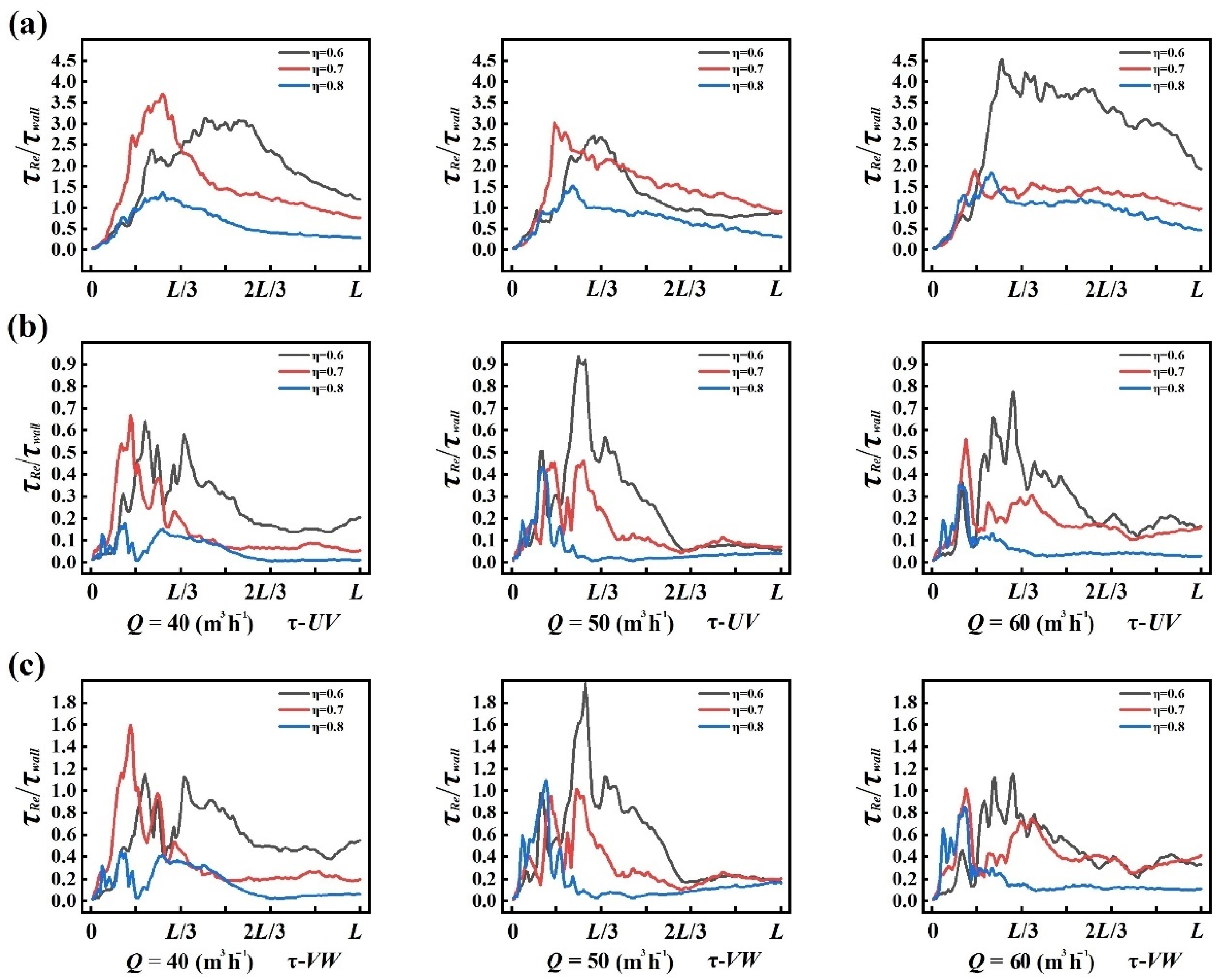
3.1.2. Reynolds Stress Characteristics

For the turbulent flow, the Reynolds stress can provide a measurement of flow momentum transportation. For spatial turbulent flow, Reynolds stress can be written as second-order correlations of two velocities of three directions at one spatial point. We adopted the types of -ρuv, -ρuw, and -ρvw and nondimensionalized them using the wall shear stress. The spatial-temporal averaged Reynolds stress along the flow is shown in Figure 3. As a total view, the Reynolds stress presented a tendency of soaring in the former region, showed resistance in middle region with a trend of decreasing, and eventually decreased in the latter region. However, the momentum transportation in the axial and radial directions (τ-UW) was obvious higher than that in other directions (τ-UV, τ-VW), and the differences were 6–14 times and 4–7 times, respectively. To sum up, in the full turbulent flow of the annular gap, the main momentum transportation of flow was in the axial and radial directions, then the axial and circular directions, and the intensity in the radial and circular directions was minor. Consequently, the main reason for the soaring—resisting—decreasing trend in the Reynolds stress along the flow was that the gap boundary disturbed the flow in the radial and axial directions, while the boundary was nearly rotationally symmetrical in the circular direction; hence, the disturbance in the circular direction was minor, leading to a minor circular component of the Reynolds stress. Still, the meridian section simplification of the annular gap flow was reasonable. The disturbance emerged at the inlet of the annular gap and spread along the flow. Because of the boundary limitation, the maximum disturbance was in the former and middle regions. Then, the disturbance began to decrease. At the flow Q = 40 m³ h⁻¹, the maxima of the three Reynolds stress values were all larger under the condition of η = 0.7 than under η = 0.6 and η = 0.8. Then, at flow Q = 60 m³ h⁻¹, the Reynolds stress was larger when η = 0.6, and the values were close at η = 0.7 and η = 0.8. However, at flow Q = 50 m³ h⁻¹, no particular diameter ratio was dominant.

3.2. Results of POD

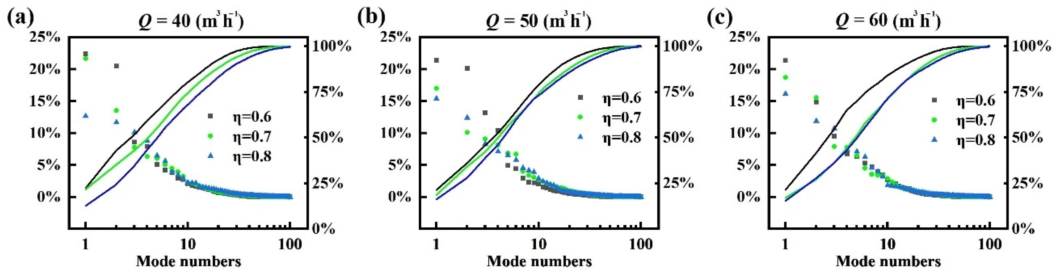
3.2.1. Turbulence Energy Contribution

Mode decomposition was performed for every combination of flow and diameter ratio conditions; each decomposition used 500 snapshots, and the time interval was 0.005 s. Different scales of turbulence structures could be captured and were ranked from high energy to low energy. The different ranks of turbulence structures and their turbulence energy contribution curves are shown in Figure 4. The scatters indicate the turbulence energy contributions of each “mode”, with values were listed on the left axis, and the curves indicate the cumulative contribution of the first several modes, with values on the right axis. As indicated, the cumulative energy curve for a lower diameter ratio converged more rapidly (η = 0.6 > η = 0.7 > η = 0.8). Under flow Q = 40 m³ h⁻¹, the first 40 modes accounted for 99% of total turbulence energy at the diameter ratio η = 0.6, the first 60 modes accounted for 99% at the diameter ratio η = 0.7, and the first 80 modes accounted for 99% at η = 0.8. However, under flow Q = 50 m³ h⁻¹, the ratio of convergence was slightly slow or fast for the corresponding diameter ratio to capture 99% of the total turbulence energy, requiring the first 46 modes (η = 0.6), the first 60 modes (η = 0.7), and the first 75 modes (η = 0.8). For flow Q = 60 m³h⁻¹, the first 40 modes (η = 0.6), the first 60 modes (η = 0.7), and the first 75 modes (η = 0.8) were required. As the scatters indicate, the lower diameter ratio had a larger turbulence energy at the same mode under the same flow; this is because of the larger characteristic length B for the lower diameter ratio.

3.2.2. The Large-Scale Coherent Structures of Flow

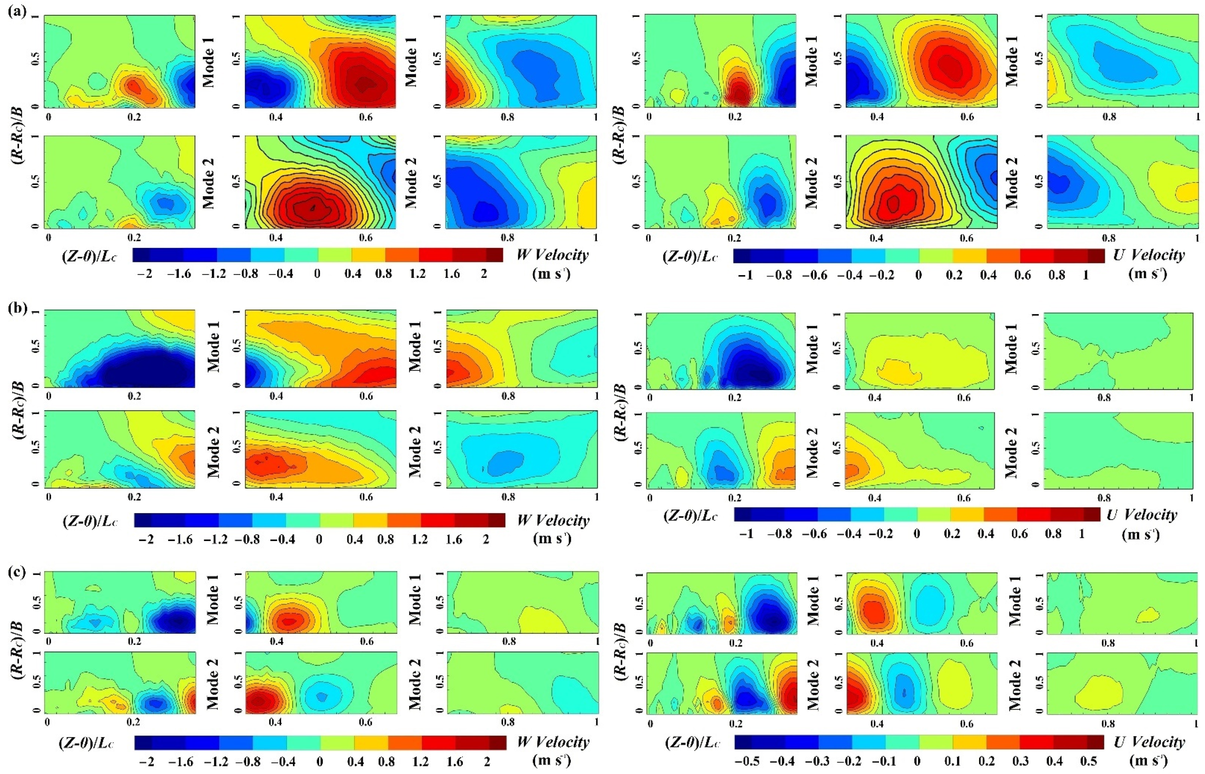
(a)

After the flow was decomposed by the POD method, the modes with high contribution were judged as the modes containing larger-scale coherent structures in the flow. These larger-scale coherent structures are normally considered as key factors of turbulence type and turbulence distribution. Hence, the first two modes for different diameter ratios are provided in Figure 5 under the flow Q = 40 m³ h⁻¹. These modes had much higher turbulence energy contributions than other modes and could thus present larger-scale coherent structures in the meridian section of flow. As shown, the coherent structures are presented by three individual components of velocity [29,30], and they show alternating positive and negative coherent vortices in the meridian sections. The magnitude of fluctuating velocity in the axial direction was 0–2 m s⁻¹, and those in the transversal direction were 0–1 m s⁻¹ (η = 0.6, η = 0.7) and 0–0.5 m s⁻¹ (η = 0.8). The diameter ratio had little influence on the axial velocity, but the transversal velocity obviously decreased with the higher diameter ratio.

(b)

In the former and middle regions of the flow, the characteristic lengths of coherent vortices rose remarkably along the flow (from 0.3 B–0.5 B to 0.9 B–1 B in the transversal direction), and the growth rate was about 1.2–1.5, nearly the same growth rate as for the length in the flow direction. Admittedly, the coherent vortices had different deformation degrees at the three diameter ratios. For the axial direction, the deformation degrees were ranked as η = 0.7 > η = 0.6 > η = 0.8, and for the transversal direction, they were ranked as η = 0.8 > η = 0.7 > η = 0.6. Nevertheless, in the latter region of the flow, the coherent vortices were easy to recognize at η = 0.6, but they nearly disappeared at η = 0.7 and η = 0.8, where the magnitude of fluctuating velocity was 1/10–1/5 that of the maximum. This indicates that at the larger diameter ratio, the larger-scale coherent structures were more focused on the regions near the inlet of the annular gap flow, and the coherent vortices were easier to break and consume near the outlet of the flow, especially at the larger diameter ratio.

(c)

Despite the turbulence energy contribution being different between the first mode and second mode, the coherent vortices had highly similar shapes for the two modes. The arbitrary coherent vortex that could be distinguished in the first mode shared a similar shape with the corresponding vortex in the second mode, only the location was a little changed and the velocity direction was reversed. This condition was like that for the first two modes of flow bypassing the cylinder (the vortices in the second mode were also a small backward distance from those in the first mode, and the direction was the opposite), so it could be considered that the coherent vortices also represented the shear vortices’ motion and growth by the main flow. However, the turbulence energy contribution was very different between the modes of annular gap flow; this was because the boundary condition was not symmetrical in the meridian section, and there was still one mode dominant.

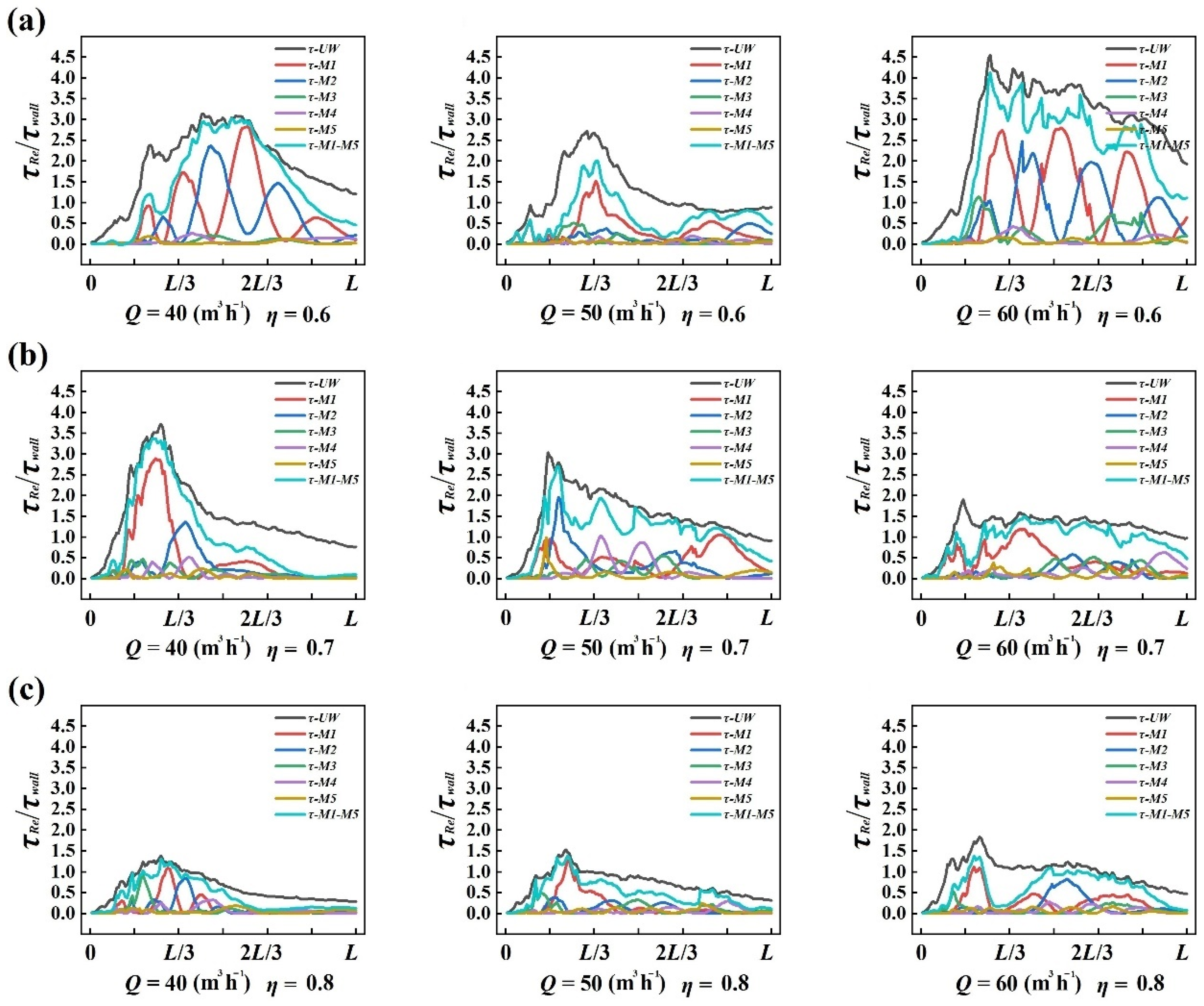
3.2.3. Reynolds Stress Contribution of Large-Scale Coherent Structures

(a)

As mentioned above, the larger-scale coherent structures might have a greater contribution to the Reynolds stress of flow; admittedly, the larger-scale coherent vortices had higher Reynolds stress values than the smaller-scale vortices. In other words, the former modes (lower-order modes) had a higher contribution to the Reynolds stress of flow, while the latter modes (higher-order modes) had a lower contribution. To verify this hypothesis, we calculated the Reynolds stress of each mode under different conditions; the results for τ-UW are provided as evidence in Figure 6 (the averaged Reynolds stress along the flow and the Reynolds stress of the first five modes). As shown, under different conditions, the first five modes captured 60–80% of the flow Reynolds stress, while the first five modes only captured about 50–70% of the turbulence energy of flow, as described in Section 3.2.1. This indicates that the POD method has a different capacity to capture the turbulence energy and the Reynolds stress, and the evidence shows that the POD method had better capacity to capture the Reynolds stress with the same number of snapshots.

(b)

As the diameter ratio increased, the value of Reynolds stress decreased; this is because the width of the gap was minor, so the momentum transportation in the radial direction of the main flow was limited. Still, from Figure 6, it can be seen that the first and second modes had a far greater contribution to the Reynolds stress than the third, fourth, and fifth modes (nearly 20–40 times larger). Some peak values of the cumulative curves for the first to fifth modes were about equal to the averaged curves, and we found that the shapes of the two curves were very similar. By calculation, the first 20 modes’ cumulative Reynolds stress curves accorded with the averaged curves, and the maximum relative error was no more than 5%; furthermore, the error was no more than 1% for the first 50 modes. To conclude, the Reynolds stress calculated by linear addition of the POD modes had better ability to describe the Reynolds stress.

3.2.4. Characteristics of Flow-Induced Vibration

The amplitude and distribution characteristics of vibration frequency are always demonstrated by spectrum maps. The power spectrum density (PSD) map is widely used for turbulence vibration [28]. The PSD function can be calculated by time—the frequency transformation for the velocities can be written as second-order correlations of one spatial point [22,23]. The PSD functions of the POD modes (with a cut-off at 99% of the turbulence energy) are provided in Figure 7 and were calculated by fast Fourier transformation (FFT) with a rectangular window. These functions could provide some frequency characteristics of the fluctuation in the flow, and it is thought that the larger-scale coherent structures make the second-order correlation higher and contribute more to the PSD value [17]. In total, the PSD functions were similar to each other to some degree: the functions had high amplitude (PSD value) in the low-frequency domain and low amplitude in the high-frequency domain, with an order of magnitude between the two amplitudes of 10⁻¹ to 10⁻². The frequency domain could be divided into three sub-domains: a low-frequency domain, a transition-frequency domain, and a high-frequency domain. Among the subdomains, the low-frequency domain (0–10 Hz) had the highest PSD values, and the values were minor under the same flow; this is because the larger diameter ratio with the gap width was minor, so the characteristic length was minor, and as a result, the scales of turbulence structures were decreased. The transition-frequency domain was 10–120 Hz; the scales of turbulence structures were not directly limited by the gap width, but the velocity was higher for a smaller gap. As a result, the PSD value was higher for a larger diameter ratio. As for the high-frequency domain (>120 Hz), the scales of turbulence structures were not influenced by characteristic length and velocity, the component of turbulence was chaotic irregular turbulence of a minor scale, and the PSD value was lower as the gap width decreased.

4. Conclusions

(a)

The Reynolds stresses of flow present a tendency of soaring in the former region, resisting some change in the middle region with a trend of decreasing, and eventually decreasing in the latter region, instead of evenly developing along the flow direction. The Reynolds stresses also indicate that the momentum transportation in the axial and radial directions (τ-UW) was obvious higher than that in other directions (τ-UV, τ-VW), and the differences were 6–14 times and 4–7 times, respectively. The flow pattern of annular gap is in more accordance with turbulence flow; laminar approximating is not suitable for the diameter ratio of the gap 0.6 to 0.8.

(b)

By proper orthogonal decomposition, the coherent structures indicated alternating positive and negative coherent vortices in the meridian sections. The diameter ratio had little influence on axial velocity, but the transversal velocity obviously decreased with a higher diameter ratio. In the former and middle regions of the flow, the characteristic length of coherent vortices showed a remarkable rise along the flow (from 0.3B–0.5B to 0.9B–1B in the transversal direction), and the growth rate was about 1.2–1.5, nearly the same growth rate as for the length in the flow direction.

(c)

The larger-scale coherent vortices of the former modes have higher Reynolds stress values than the smaller-scale vortices of the latter modes. The first five modes captured 60–80% of the flow Reynolds stress, while the first five modes only captured about 50–70% of the turbulence energy of the flow. The first 20 modes’ cumulative Reynolds stress curves accorded with the averaged curves, and the maximum relative error was no more than 5%. The Reynolds stress calculated by linear addition of the POD modes had a better ability to describe the Reynolds stress.

(d)

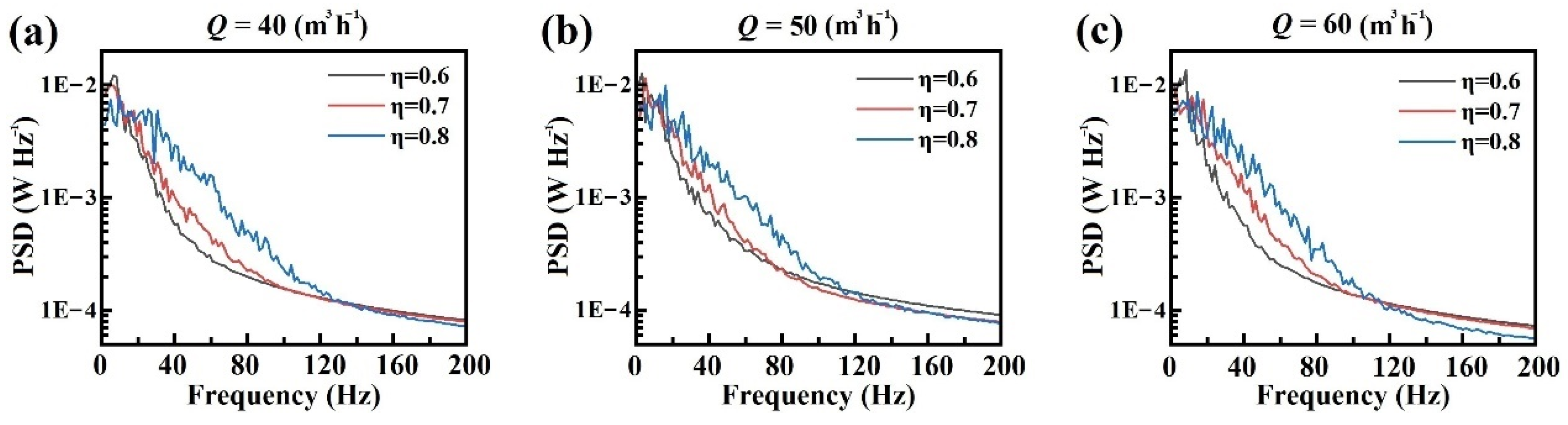
The power spectrum density functions of the flow show the frequency distribution of the flow-induced vibration: the functions had high amplitude in the low-frequency domain and low amplitude in the high-frequency domain, with an order of magnitude between the two amplitudes of 10⁻¹ to 10⁻². The frequency domain could be divided into three subdomains: a low-frequency domain (0–10 Hz), a transition-frequency domain (10–120 Hz), and a high-frequency domain (>120 Hz). The gap width or averaged velocity has little influence on the frequency in the low-frequency domain. The frequency is higher at a smaller gap width in the middle-frequency domain, but the condition is opposite in the high-frequency domain.

References

1. Zhou, R.; Meng, L.; Yuan, X.; Qiao, Z. Research and Experimental Analysis of Hydraulic Cylinder Position Control Mechanism Based on Pressure Detection. Machines 2022, 10, 1. [Google Scholar] [CrossRef]
2. Dzyura, V.; Maruschak, P. Optimizing the Formation of Hydraulic Cylinder Surfaces, Taking into Account Their Microrelief Topography Analyzed during Different Operations. Machines 2021, 9, 116. [Google Scholar] [CrossRef]
3. Yin, L.; Deng, W.; Yang, X.; Yao, J. Finite-Time Output Feedback Control for Electro-Hydraulic Servo Systems with Parameter Adaptation. Machines 2021, 9, 214. [Google Scholar] [CrossRef]
4. Kalligeros, S.S. Predictive Maintenance of Hydraulic Lifts through Lubricating Oil Analysis. Machines 2014, 2, 1. [Google Scholar] [CrossRef]
5. Li, L.; Lin, Z.; Jiang, Y.; Yu, C.; Yao, J. Valve Deadzone/Backlash Compensation for Lifting Motion Control of Hydraulic Manipulators. Machines 2021, 9, 57. [Google Scholar] [CrossRef]
6. Liu, H.; Graze, H.R. Lift and Drag on Stationary Capsule in Pipeline. J. Hydraul. Eng. 1983, 109, 28–47. [Google Scholar] [CrossRef]
7. Xu, X.; Zhu, B.; Zhang, J.; Wang, C. The Research of the Concentric Ring Slit Flow. J. Anhui Univ. Sci. Technol. Nat. Sci. 2004, 24, 40–42. (In Chinese) [Google Scholar] [CrossRef]
8. Li, Y.; Sun, X.; Zhang, X. Experimental study of the wheeled capsule motion inside hydraulic pipeline. Adv. Mech. Eng. 2019, 11, 168781401984406. [Google Scholar] [CrossRef]
9. Li, Y.; Gao, Y.; Sun, X.; Zhang, X. Study on Flow Velocity during Wheeled Capsule Hydraulic Transportation in a Horizontal Pipe. Water 2020, 12, 1181. [Google Scholar] [CrossRef] [Green Version]
10. Li, Y.; Sun, X. Mathematical Model of the Piped Vehicle Motion in Piped Hydraulic Transportation of Tube-Contained Raw Material. Math. Probl. Eng. 2019, 2019, 3930691. [Google Scholar] [CrossRef]
11. Chen, X.; Gao, W.; Zhang, J. Analysis of Spherical Interstitial Flow Characteristics of Component in the Piston Pump. Chin. Hydraul. Pneum. 2021, 45, 87–97. (In Chinese) [Google Scholar] [CrossRef]
12. Sun, Q.; Yu, L. Study on Dynamic Coefficients of Concentric Rotor in Finite- Length Large Gap Annular Flow. Tribology 2001, 21, 473–477. (In Chinese) [Google Scholar] [CrossRef]
13. Shcherba, V.; Shalai, V.; Pustovoy, N.; Pavlyuchenko, E.; Gribanov, S.; Dorofeev, E. Calculation of the Incompressible Viscous Fluid Flow in Piston Seals of Piston Hybrid Power Machines. Machines 2020, 8, 21. [Google Scholar] [CrossRef] [Green Version]
14. Geng, T.; Schoen, M.A.; Kuznetsov, A.V.; Roberts, W.L. Combined Numerical and Experimental Investigation of a 15-cm Valveless Pulsejet. Flow Turbul. Combust. 2007, 78, 17–33. [Google Scholar] [CrossRef]
15. Poncet, S.; Haddadi, S.; Viazzo, S. Numerical modeling of fluid flow and heat transfer in a narrow Taylor–Couette–Poiseuille system. Int. J. Heat Fluid Flow 2011, 32, 128–144. [Google Scholar] [CrossRef] [Green Version]
16. Kareem, M.K.; Abed, W.M.; Dawood, H.K. Numerical simulation of hydrothermal behavior in a concentric curved annular tube. Heat Transf. 2020, 49, 2494–2520. [Google Scholar] [CrossRef]
17. Rehimi, F.; Aloui, F. Synchronized analysis of an unsteady laminar flow downstream of a circular cylinder centred between two parallel walls using PIV and mass transfer probes. Exp. Fluids 2011, 51, 1–22. [Google Scholar] [CrossRef]
18. Ali, N.; Cortina, G.; Hamilton, N.; Calaf, M.; Cal, R.B. Turbulence characteristics of a thermally stratified wind turbine array boundary layer via proper orthogonal decomposition. J. Fluid Mech. 2017, 828, 175–195. [Google Scholar] [CrossRef]
19. Yeh, S.T.; Wang, X.; Sung, C.L.; Mak, S.; Chang, Y.H.; Zhang, L.; Wu, C.F.J. Common Proper Orthogonal Decomposition-Based Spatiotemporal Emulator for Design Exploration. AIAA J. 2018, 56, 2429–2442. [Google Scholar] [CrossRef] [Green Version]
20. Chu, S.; Xia, C.; Wang, H.; Fan, Y.; Yang, Z. Three-dimensional spectral proper orthogonal decomposition analyses of the turbulent flow around a seal-vibrissa-shaped cylinder. Phys. Fluids 2021, 33, 025106. [Google Scholar] [CrossRef]
21. Premaratne, P.; Tian, W.; Hu, H. A Proper-Orthogonal-Decomposition (POD) Study of the Wake Characteristics behind a Wind Turbine Model. Energies 2022, 15, 3596. [Google Scholar] [CrossRef]
22. Michelis, T.; Kotsonis, M. Interaction of an off-surface cylinder with separated flow from a bluff body leading edge. Exp. Therm. Fluid Sci. 2015, 63, 91–105. [Google Scholar] [CrossRef]
23. Zhang, H.T.; Zhang, J.M.; Han, C.; Ye, T.H. Coherent Structures of Flow Fields in Swirling Flow Around a Bluff-body Using Large Eddy Simulation. Acta Aeronaut. Astronaut. Sin. 2014, 35, 1854–1864. (In Chinese) [Google Scholar] [CrossRef]
24. Yue, Y.; Zhang, X.; Liu, L.; Liang, l.; Zhu, B. Evaluate Method Research of PIV System Measurement Error. Comput. Meas. Control. 2018, 26, 255–259. [Google Scholar] [CrossRef]
25. Neal, D.R.; Sciacchitano, A.; Smith, B.L.; Scarano, F. Collaborative framework for PIV uncertainty quantification: The experimental database. Meas. Sci. Technol. 2015, 26, 074003. [Google Scholar] [CrossRef]
26. Lumley, J.L. Similarity and the Turbulent Energy Spectrum. Phys. Fluids 2004, 10, 855–858. [Google Scholar] [CrossRef]
27. Sirovich, L. Turbulence and the dynamics of coherent structures: Part 1: Coherent structures. Q. Appl. Math. 1987, 45, 561–571. [Google Scholar] [CrossRef] [Green Version]
28. Sieber, M.; Paschereit, C.O.; Oberleithner, K. Spectral proper orthogonal decomposition. J. Fluid Mech. 2016, 792, 798–828. [Google Scholar] [CrossRef] [Green Version]
29. Liu, W.; Guo, D.; Zhang, Z.; Yang, G. Study of dynamic characteristics in wake flow of High-speed train based on POD. J. China Railw. Soc. 2020, 42, 49–57. (In Chinese) [Google Scholar] [CrossRef]
30. Zou, Y.; Liang, S.; Zou, L. Reconstruction of fluctuating wind pressure field by applying POD of eigenvector correction. China Civ. Eng. J. 2010, 43, 305–309. (In Chinese) [Google Scholar]
Figure 1. Schematics of the experimental model and annular gap flow: (a,b) schematics of annular gap and size parameters of the capsule; (c) components of the experimental system; (d,e) setup of the PIV system and schematic of the meridian section.
Machines 10 00645 g001
Figure 2. Averaged velocity of a meridian section under flow Q = 40 (m3 h−1): (a) contour for the gap width B = 20 × 10−3 m, η = 0.8; (b) contour for the gap width B = 15 × 10−3 m, η = 0.7; (c) contour for the gap width B = 10 × 10−3 m, η = 0.6. The contours show the velocity magnitude, and the arrows show the velocity direction.
Machines 10 00645 g002
Figure 3. Reynolds stress of a meridian section along the flow: (a) the Reynolds stress τ-UW at three flows; (b) the Reynolds stress τ-UV at three flows; (c) the Reynolds stress τ-VW at three flows. The Reynolds stresses are nondimensionalized by the wall shear stresses.
Machines 10 00645 g003
Figure 4. Turbulent energy contributions of each mode and the cumulative contribution: (a) the contribution curves at the flow Q = 40 m3h−1; (b) the contribution curves at the flow Q = 50 m3h−1; (c) the contribution curves at the flow Q = 60 m3h−1. The turbulent energy contributions are the scatters and correspond to the left axis; the cumulative contributions are the curves and correspond to the right axis.
Machines 10 00645 g004
Figure 5. Large-scale coherent vortices of the first and second modes at Q = 40 (m3 h−1): (a) contour of structures of velocity at η = 0.6; (b) contour of structures of velocity at η = 0.7; (c) structures of velocity at η = 0.8.
Machines 10 00645 g005
Figure 6. Reynolds stress contribution curves of the first five modes: (a) the contribution curves for η = 0.6 at three flows; (b) the contribution curves for η = 0.7 at three flows; (c) the contribution curves for η = 0.8 at three flows.
Machines 10 00645 g006
Figure 7. Power spectrum density functions of the meridian section: (a) the function curves at flow Q = 40 m3h−1; (b) the function curves at flow Q = 50 m3h−1; (c) the function curves at flow Q = 60 m3h−1.
Machines 10 00645 g007