Article

Intelligent Diagnosis Method for Mechanical Faults of High-Voltage Shunt Reactors Based on Vibration Measurements

College of Energy and Electrical Engineering, Hohai University, Nanjing 211100, China
*
Author to whom correspondence should be addressed.
Machines 2022, 10(8), 627; https://doi.org/10.3390/machines10080627
Submission received: 22 June 2022 / Revised: 21 July 2022 / Accepted: 27 July 2022 / Published: 29 July 2022

Abstract

:
Aiming at the difficulty of accurately identifying latent mechanical faults inside high-voltage shunt reactors (HVSRs), this paper proposes a new method for HVSR state feature extraction and intelligent diagnosis. The method integrates a modified complementary ensemble empirical mode decomposition (CEEMD)–permutation entropy–CEEMD (MCPCEEMD) method, mutual information theory (MI), multiscale fuzzy entropy (MFE), and an improved grasshopper optimization algorithm to optimize the probabilistic neural network (IGOA-PNN) model. First, we introduce MCPCEEMD for suppressing modal aliasing to decompose the HVSR raw vibration signals. Then, the correlation degree between the obtained intrinsic mode function (IMF) components and the HVSR original vibration signals is judged through MI, and the IMF with the highest correlation is selected for feature extraction. Furthermore, this study uses MFE to quantify the selected IMF. Finally, we employ piecewise inertial weights to improve GOA to select the best smoothing factor for PNN, and use the optimized IGOA-PNN model to identify feature subsets. The experimental results show that the proposed method can successfully diagnose different types and degrees of HVSR mechanical faults, and the identification accuracy rate reaches more than 98%. The high recognition accuracy of the proposed method is helpful for the state detection and field application of HVSRs.

1. Introduction

A high-voltage shunt reactor (HVSR) is an important reactive power compensation device in a power grid that plays an irreplaceable role in absorbing capacitive reactive power, limiting the rise of power frequency voltage, and reducing line losses [1,2,3]. Under the long-term action of electromagnetic force and mechanical force, the internal components of an HVSR are prone to failure. For example, silicon steel sheets are worn out, windings and iron cores become loose, spacers are dropped, and windings are deformed [4,5,6,7]. If an HVSR fault is not discovered in time, it will seriously threaten the security of the power grid and may cause large-scale power outages in the power grid. Therefore, it is very important to find a method that can monitor and accurately diagnose HVSR faults in real time to ensure the safety and stability of the power grid.
The vibration method has the advantages of no electrical connection with the HVSR, safety, reliability, high sensitivity, and real-time monitoring, and has received extensive attention from scholars [8,9,10]. The key to HVSR mechanical fault diagnosis based on vibration signals depends on the accurate extraction of vibration signal feature quantities. The HVSR vibration signal has obvious nonlinear and nonstationary characteristics [11,12]. In a complex noise environment, effectively extracting the state information contained in the HVSR vibration signal is a challenging problem. Numerous popular signal-processing methods, such as wavelet transform (WT) [13] and empirical mode decomposition (EMD) [14], are applied to the analysis and feature extraction of vibration signals. However, in essence, WT is a kind of Fourier transform, which has problems such as insufficient adaptability and energy leakage. EMD can perform adaptive multiresolution decomposition in combination with signal characteristics, but there are problems of end effect and mode aliasing. To reduce the phenomenon of mode aliasing, Yeh et al. [15] described a complementary ensemble empirical mode decomposition (CEEMD) method. CEEMD effectively alleviates the modal confusion phenomenon existing in EMD, but CEEMD is extremely strict in the selection of the number of decomposition iterations and auxiliary white noise, which may generate false components and affect the final feature extraction accuracy [16]. Therefore, to solve the modal aliasing problem, this study adopts a modified CEEMD–permutation entropy (PE) –CEEMD (MCPCEEMD) signal decomposition method to decompose and extract features of HVSR vibration signals.
Multiple intrinsic mode function (IMF) components can be obtained, depending on the decomposition of the vibration signal by MCPCEEMD. However, the correlations of multiple IMFs with the original vibration signal are different, and there is a phenomenon of feature redundancy. To effectively extract feature quantities, we need to analyze the correlation of multiple IMFs. At present, there are many approaches to analyzing the similarity or change trend between two signals, such as the Pearson correlation coefficient (PCC) [17], Mann–Kendall test method (M-K) [18], and mutual information (MI) [19]. However, PCC may lead to spurious correlations, and M-K is limited to a single time series. Therefore, this paper uses MI to calculate the correlation between the IMF and the raw vibration signal to obtain the IMF with the highest degree of correlation. It should be noted that the fault feature information contained in the IMF component is still not obvious, and further quantitative calculation is needed. The entropy algorithm [20] and fractal dimension [21] are the main fault information quantification methods. As an active method to estimate the dynamic properties of complex time series, entropy is widely used in the quantitative solution of fault information [22]. Multiscale fuzzy entropy (MFE), as a kind of entropy, contains rich temporal pattern information [23]. Therefore, this paper uses MFE to quantify the IMF component with the highest correlation degree to quantitatively mirror the state characteristics of HVSRs.
The appropriate diagnostic method is used to recognize different kinds of mechanical faults in the HVSR after obtaining a quantified feature set. Considering the strong decision-making ability of probabilistic neural networks (PNNs) under the condition of small samples [24], this study introduces the PNN classification algorithm to realize the automatic identification of HVSR mechanical faults. To exert the best performance of the PNN, we use an improved grasshopper optimization algorithm (IGOA) to optimize the key parameters of the PNN to obtain high-precision classification results.
To identify HVSR mechanical faults more accurately, we propose an HVSR fault diagnosis method based on the combined application of MCPCEEMD-MFE and the IGOA-PNN model. The primary contributions of this study are summarized as follows:
(1)
Aiming at the problem of modal aliasing, we introduce permutation entropy (PE) into CEEMD to remove noise and abnormal components that cause mode confusion so as to obtain more effective feature quantities.
(2)
To reduce the redundancy of features and improve the effectiveness of features, this paper uses MI to calculate the correlation between the IMF components and the original vibration signal, and takes the IMF component with the highest correlation as the feature quantity. Furthermore, MFE is used to quantify features to quantitatively reflect different fault types and fault degrees of HVSR.
(3)
To improve the accuracy of fault feature recognition, an IGOA-PNN fault recognition model is proposed in this study. The smoothing factor of the PNN is optimized with the optimized IGOA to achieve the best classification.
The rest of this study is organized as follows. Section 2 introduces the implementation of MCPCEEMD, MI, MFE, and the IGOA-PNN model. Section 3 describes the proposed fault diagnosis method in detail. Section 4 describes the experimental verification and discusses the results in detail. Conclusions are given in Section 5.

2. Research Methodology

In this section, we elaborate the MCPCEEMD proposed in this paper and briefly demonstrate the existing MI theory and MFE calculation principle. Furthermore, we introduce the improved GOA method proposed in this paper and the computational steps of the proposed IGOA-PNN model.

2.1. MCPCEEMD Method

To further suppress modal confusion, this paper uses the PE to evaluate multiple IMF components decomposed by CEEMD. We discard the IMF components whose PE value (VPE) is greater than the set threshold to eliminate noise and abnormal components that cause pattern confusion. In [25], the calculation process of PE is given in detail. It has been concluded that the smaller the VPE is, the more regular the corresponding time series, representing a periodic signal; in contrast, the larger the VPE is, the more random the time series, representing noise [25].
For an HVSR raw vibration signal X ( t ) , the flow chart of MCPCEEMD is shown in Figure 1, and the specific decomposition steps are as follows [15].
Step 1: Perform CEEMD decomposition on the HVSR original vibration signal X ( t ) to obtain the IMF components I M F i ( t ) ( i = 1 , 2 , , N ) .
Step 2: Calculate the VPE of the IMF i ( t ) component.
Step 3: Determine whether the IMF is a normal signal. If the VPE of the IMF i ( t ) component is less than 0.65, it is determined to be a normal component and reserved; otherwise, it is identified as an abnormal IMF component, eliminated, and returned to Step 2.
Step 4: Iterate until the IMF p ( t ) component is not an abnormal signal, where p represents the pth IMF component.
Step 5: Discard the first p-1 abnormal signals from X ( t ) :
r ( t ) = X ( t ) j = 1 p 1 IMF j ( t )
where r ( t ) is the residual signal, and IMF j ( t ) is the jth abnormal IMF component.
Step 6: Perform CEEMD [15] decomposition again on r ( t ) to extract the required IMF components.

2.2. Mutual Information Introduction

MI theory [19] can measure the amount of information one variable contains in another random variable. In information theory, MI is used to judge the correlation between two signals. Assuming two random variables Q and V, if their joint probability density is p(q, v) and the marginal probability density distribution is p(q) and p(v), then the calculation formula of mutual information I(Q; V) is [19]:
I ( Q ; V ) = q Q v V p ( q , v ) log p ( q , v ) p ( q ) p ( v )
Formula (2) shows that the larger the mutual information value is, the stronger the correlation between the two random variables.

2.3. Multiscale Fuzzy Entropy

Fuzzy entropy (FE) can effectively reflect the complexity and instability of time series [26]. Assuming that a time series composed of N points is { u ( i ) , 1 i N } , the calculation expression of its FE value is [27]:
FuzzyEn ( m , n , r ) = lim N [ ln ϕ m ( n , r ) ln ϕ m + 1 ( n , r ) ]
{ ϕ m ( n , r ) = 1 N m i = 1 N m ( 1 N m 1 j = 1 , j i N m e ( d i j m / r ) n ) d i j m = max k ( 0 , m 1 ) { | u ( i + k ) u 0 ( i ) ( u ( j + k ) u 0 ( j ) ) | } ( i , j = 1 , 2 , , N m , i j )
where d i j m is the maximum value of the distance difference between the corresponding elements in the two m-dimensional vectors; m is the embedding dimension; n and r are the gradient and width of the fuzzy function boundary, respectively; and u 0 ( i ) and u 0 ( j ) are the average of i points and the average of j points in the time series, respectively.
MFE introduces the concept of multiscale into FE [23], which effectively overcomes the defect of measuring time series with a single FE value. MFE is defined as follows: The time series { u ( i ) , 1 i N } of N points is coarse-grained to form a new time series:
χ j ( τ ) = 1 τ i = ( j 1 ) τ + 1 j τ u i 1 j N τ
where τ is the scale factor.

2.4. Proposed IGOA-PNN Model

In this section, we introduce the IGOA-PNN model proposed in this paper and the improvement strategy of GOA in detail. Specifically, aiming at the highest diagnostic accuracy, we use the IGOA algorithm to select the best smoothing factor of the PNN to obtain the IGOA-PNN model. It is worth noting that in order to improve the optimization accuracy of GOA, we introduce the piecewise inertia coefficient into the position update of the locust.

2.4.1. Probabilistic Neural Network

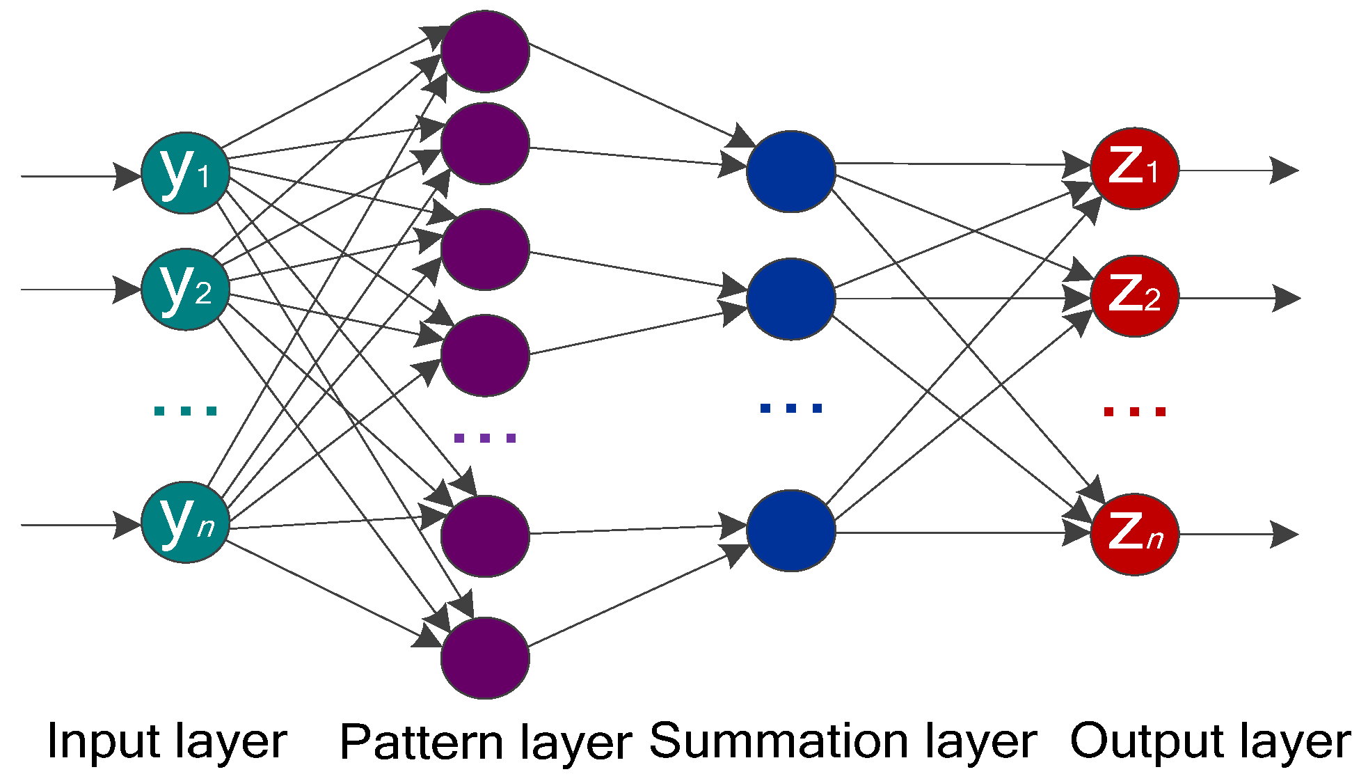
As an improved artificial neural network, PNN is essentially a parallel classification algorithm based on the Bayesian minimum risk criterion [28]. The network topology of the PNN is shown in Figure 2, including the input layer, pattern layer, summation layer and output layer.
Assuming that there are E samples in the dataset, these samples can be divided into M categories, and assuming that both the input sample and the training sample contain η features, then the input sample feature vector Y can be represented as an η -dimensional Y = [ y 1 , y 2 , , y η ] . The main task of the input layer is to receive input sample data and pass it to the pattern layer for processing. The pattern layer matches the received Y with each pattern category in a nonlinear mapping relationship. The Gaussian function of the ith class and the jth mode unit calculated by the pattern layer is [28]:
Φ i j ( Y ) = 1 ( 2 π ) η / 2 σ η exp [ ( Y Y i j ) T ( Y Y i j ) 2 σ 2 ]
where i = 1 , 2 , , M , j = 1 , 2 , , E i , E i represents the number of samples in the ith category, E i meets i = 1 M E i = E , Y i j represents the jth sample of the ith class, and σ is the smoothing factor.
Then, the output of the pattern layer is passed to the summation layer. The output of the ith summation unit in the summation layer can be described as:
f i ( Y ) = 1 N i j = 1 N i Φ i j ( Y )
where the f i ( Y ) input vector Y is classified to the maximum likelihood of the ith class.
Finally, the output layer is the decision layer based on the Bayes optimal decision rule. The classification of the input vector Y by the output layer can be expressed as:
z = arg max i Γ [ f i ( Y ) ] = { i | ς Γ , f ς ( Y ) f i ( Y ) }
where Γ = [ 1 , 2 , , M ] , and z is the category of the input vector Y. It can be seen from the calculation process of the above PNN that the topology of the PNN is simple, and there are no training rules and connection allocation weights of the connection layer. However, there is a challenging problem in using PNN for signal recognition, namely, how to choose an appropriate smoothing factor σ to enhance the classification performance. This issue will be discussed in Section 2.4.3.

2.4.2. Proposed IGOA Algorithm

The GOA was proposed by Saremi et al. [29], and its basic idea originated from the foraging behavior of locust swarms. The GOA has low computational complexity and fast convergence speed and has been widely used in solving optimization problems [30,31,32,33]. The principle and computational steps of the GOA are introduced in detail in [29]. Here, in view of the problem that the GOA is prone to falling into a local optimum, this paper proposes an improved strategy for traditional GOA.
To improve the optimization accuracy of the GOA and prevent it from falling into a local optimum, this study introduces a piecewise inertia weight coefficient into the locust position update formula. The formula for updating the position of the kth locust in the dth dimension space in the traditional GOA is shown in Formula (9):
W k d = c ( l = 1 , l k R c b u d b v d 2 s ( | w l d w k d | ) w l d w k d d k l ) + T t a r d
where W k d is the position of the kth locust in the dth dimension space; c = c max t c max c min T ; c max = 1 , c min = 0.0004 ; t is the current iteration number; T is the maximum iteration number; R is the number of locusts; b u d and b v d represent that the upper bound of the locust in the d-dimensional space is 2 and the lower bound is 0.01, respectively; s is the social force; w l d and w k d are the ith and kth locusts in the d-dimensional space, respectively; d k l = | w l d w k d | is the distance between the lth locust and the kth locust; and T t a r d is the position of the locust with the best fitness value in the d-dimensional space, that is, the target position of the locust.
In this paper, the update formula for introducing the inertia weight coefficient w into the locust position is:
W k d = c ( l = 1 , l k R c b u d b v d 2 s ( | w l d w k d | ) w l d w k d d k l ) + w T t a r d
In the initial moment of GOA optimization, the dispersion degree of grasshoppers is relatively high, and a larger value of w is beneficial to enhance the overall exploration ability of grasshoppers. In the later period of the GOA, the aggregation degree of grasshoppers is high, and a small value of w is beneficial to grasshoppers searching in a local range. Assuming that the fitness value of an individual grasshopper in the tth iteration is f w i ( t ) , the average fitness value of individual grasshoppers is calculated as f a v = 1 R i = 1 R f w i . When the individual fitness value is less than f a v , the corresponding average fitness value is f a v 1 ; when the individual fitness value is greater than f a v , the corresponding average fitness value is f a v 2 . We compare the f w i ( t ) of each grasshopper with f a v 1 and f a v 2 and divide the grasshopper population into three grades with distinctive inertia weights. The segmentation value strategy of w is:
(1)
When f w i ( t ) is less than f a v 1 , w is 0.9.
(2)
When f w i ( t ) is greater than f a v 1 and less than f a v 2 , w belongs to [ 0.7 , 0.9 ) .
(3)
When f w i ( t ) is greater than f a v 2 , w is 0.2.

2.4.3. IGOA-PNN

The recognition results of the PNN model are greatly affected by the smoothing factor, and an appropriate smoothing factor is the key to ensuring the classification and recognition results [34]. Therefore, this paper optimizes the value of the smoothing factor in the PNN. In this paper, the IGOA is used to select the best smoothing factor of the PNN, and the fitness function is constructed as:
max f i t n e s s = T r u e n u m T o t a l n u m × 100 %
where T r u e n u m is the number of correctly classified samples, and T o t a l n u m is the total number of samples. The computational flow chart of the proposed IGOA-PNN model is shown in Figure 3.

3. Proposed Framework

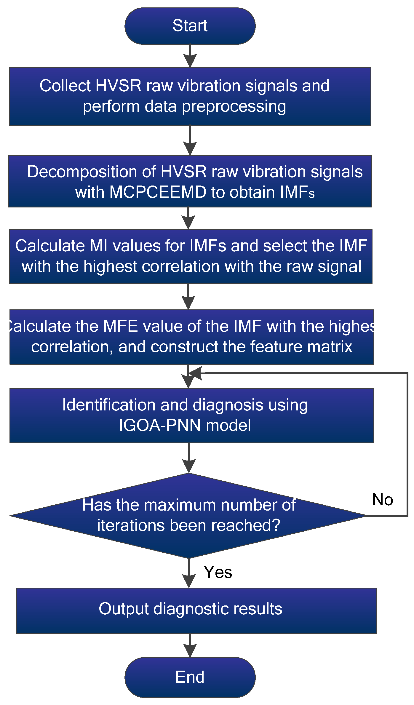
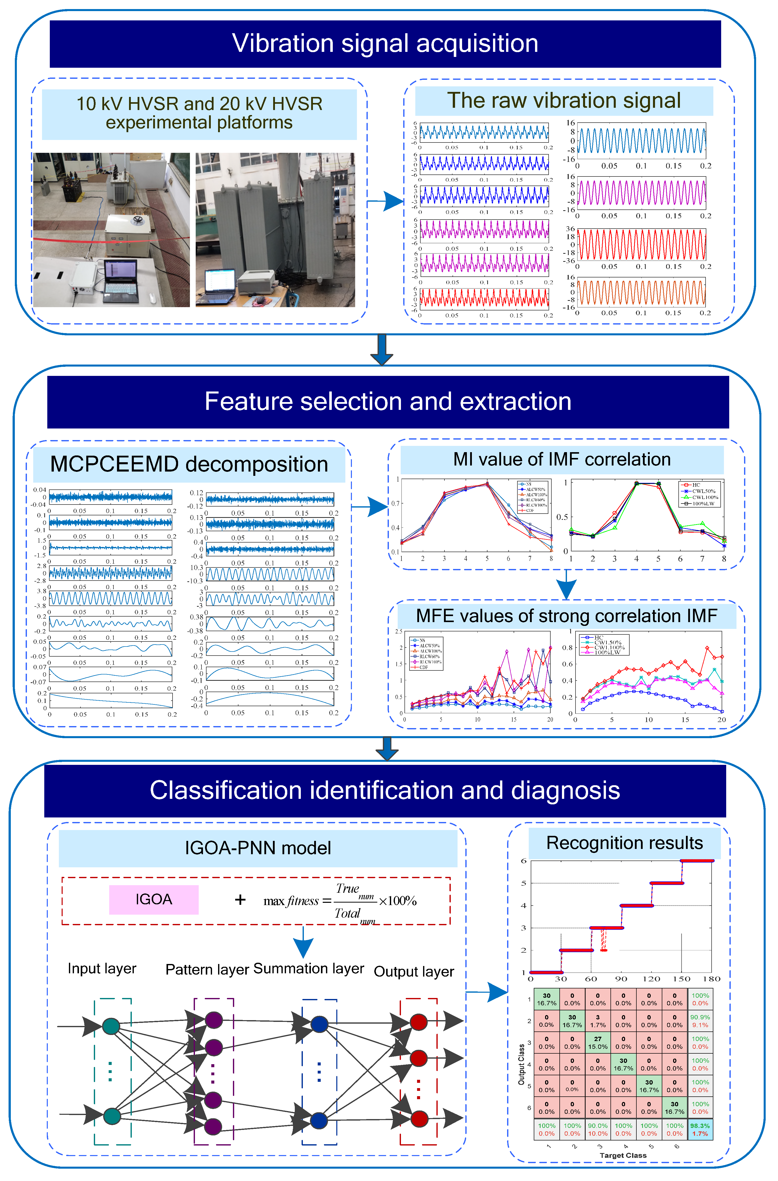
In this study, we propose a method to obtain vibration characteristics from vibration signals of HVSR operating states to detect and diagnose HVSR internal mechanical faults. To achieve this goal, four key techniques, including improved MCPCEEMD, MI, MFE, and the optimized IGOA-PNN model, are integrated into the proposed method. The flowchart and working structure of the proposed method are shown in Figure 4 and Figure 5, respectively, and the specific implementation process is described as follows.
Step 1: Collect HVSR vibration signals and perform data preprocessing.
Step 2: Use MCPCEEMD to decompose the HVSR vibration signal to obtain the IMF components.
Step 3: Calculate the MI value of each IMF component, and select the IMF component with the highest correlation.
Step 4: Calculate the MFE values of the highest correlated IMF components at different scale factors and construct feature matrices from them.
Step 5: Input the feature matrix into the trained IGOA-PNN model for identification and diagnosis.
Step 6: Output the decision result for the HVSR vibration signals.

4. Experiment Verification and Discussion

This section presents two case studies to examine the effectiveness and generality of the proposed MCPCEEMD-MFE-IGOA-PNN method. In the two cases of 10 kV and 20 kV HVSRs, we simulate a variety of typical HVSR internal mechanical faults and obtain vibration signal datasets under different operating conditions. This study analyzes the experimental results of typical failures of HVSRs and evaluates the excellent performance of the proposed method by comparison.

4.1. Case 1: 10 kV HVSR Experimental Verification and Discussion

4.1.1. Experimental Platform and Data Collection

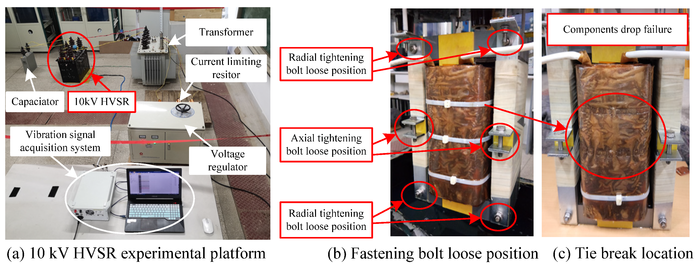
In this case, the vibration signals of typical 10 kV HVSR faults are used to verify the proposed method. The 10 kV HVSR experimental platform mainly includes a 10 kV HVSR, capacitor, transformer, voltage regulator, and vibration signal acquisition system, as shown in Figure 6a. The model of the vibration signal acquisition system is DH5922D. The model of the acceleration sensor is 1A212E, and its sensitivity is 50   mv / ( m · s 2 ) . The sampling frequency of the HVSR vibration signal is set to 20 kHz, each sampling time is 10 s, and each working condition is repeatedly sampled five times to increase the sample size. We simulate five typical fault states and normal states of the HVSR, and the fault setting positions are shown in Figure 6b,c. Table 1 presents the fault types and corresponding category labels. In this case, we use two broken winding ties to simulate the fall fault of the HVSR winding spacer.
In this study, the vibration signal of the HVSR box is collected by an array method, and a total of 53 measuring points are arranged to obtain detailed and accurate original vibration data. Figure 7a presents the measuring point layout and numbering. In this case, 3072 sample points are divided into one group, and 100 groups are randomly selected for each state for feature extraction. In this paper, measuring point No. 42 with high vibration intensity is selected for analysis. The position of measuring point No. 42 is shown in Figure 7b. Figure 8 shows the waveforms of vibration signals under six working conditions at measuring point No. 42.

4.1.2. Analysis of Results

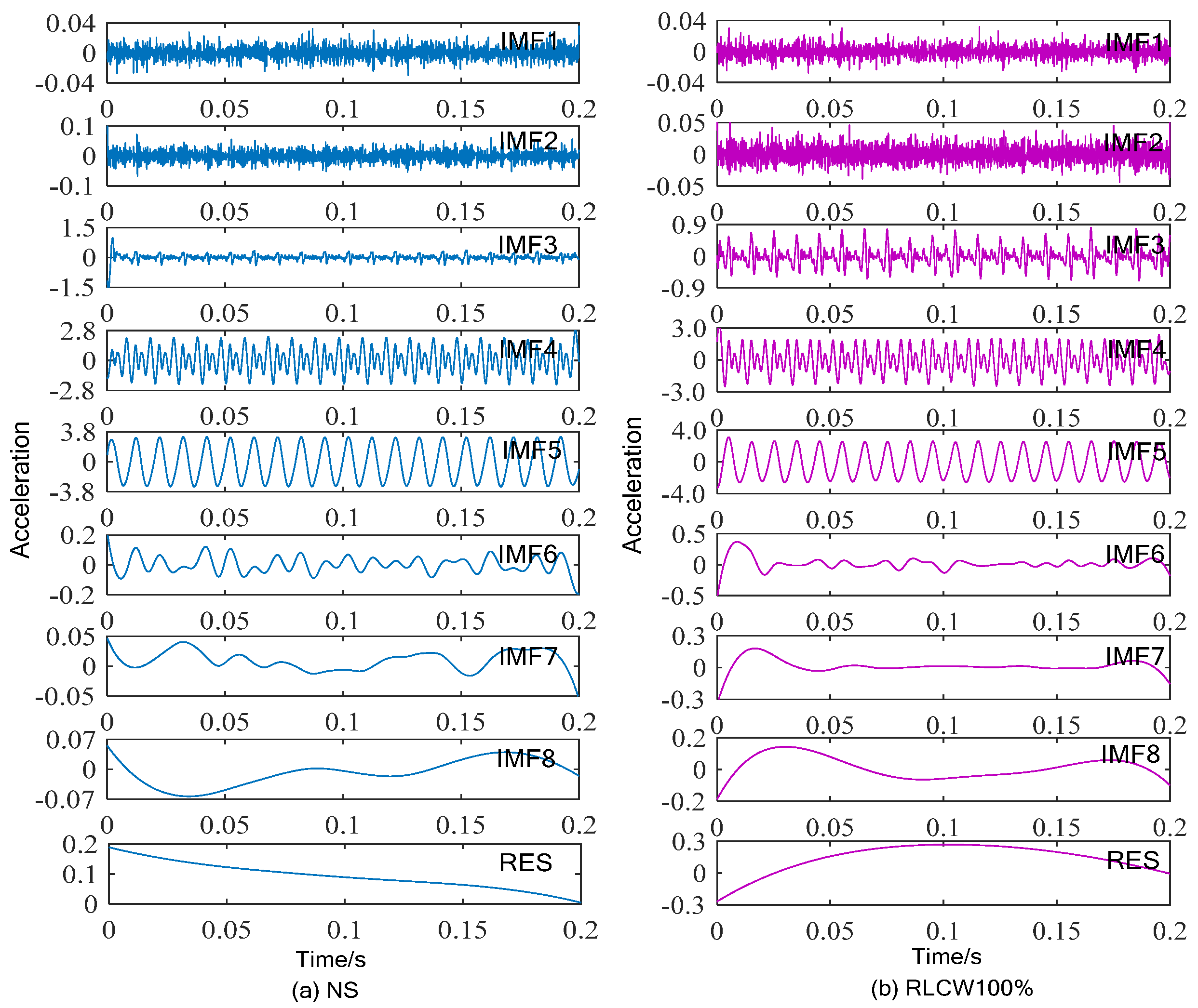
After acquiring the HVSR vibration signal, this paper utilizes the proposed MCPCEEMD-MFE-IGOA-PNN model for identification and diagnosis, which is presented in Section 3. First, MCPCEEMD is used to decompose the HVSR raw vibration signal. To control the decomposition error, this paper sets the white noise logarithm Ne to 50 and the white noise standard deviation Nstd to 0.2. At the same time, we set the threshold VPE of PE as 0.65. Considering the readability of the article, this article only shows the MCPCEEMD results of measuring point No. 42 in the NS and RLCW100% cases, as shown in Figure 9. They contain eight IMF components and a residual term.
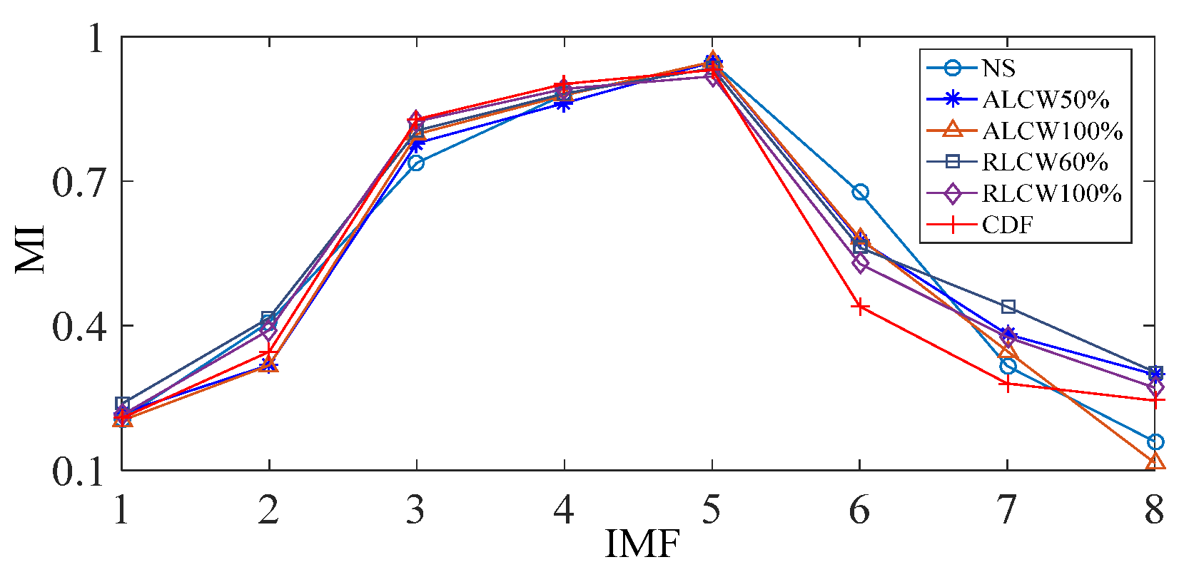
Then, we calculate the MI value of each IMF component obtained by MCPCEEMD. The MI value can effectively reflect the degree of correlation between the IMF component and the original vibration signal. Figure 10 displays the MI value variation curves of different IMF components under different working conditions of the HVSR.
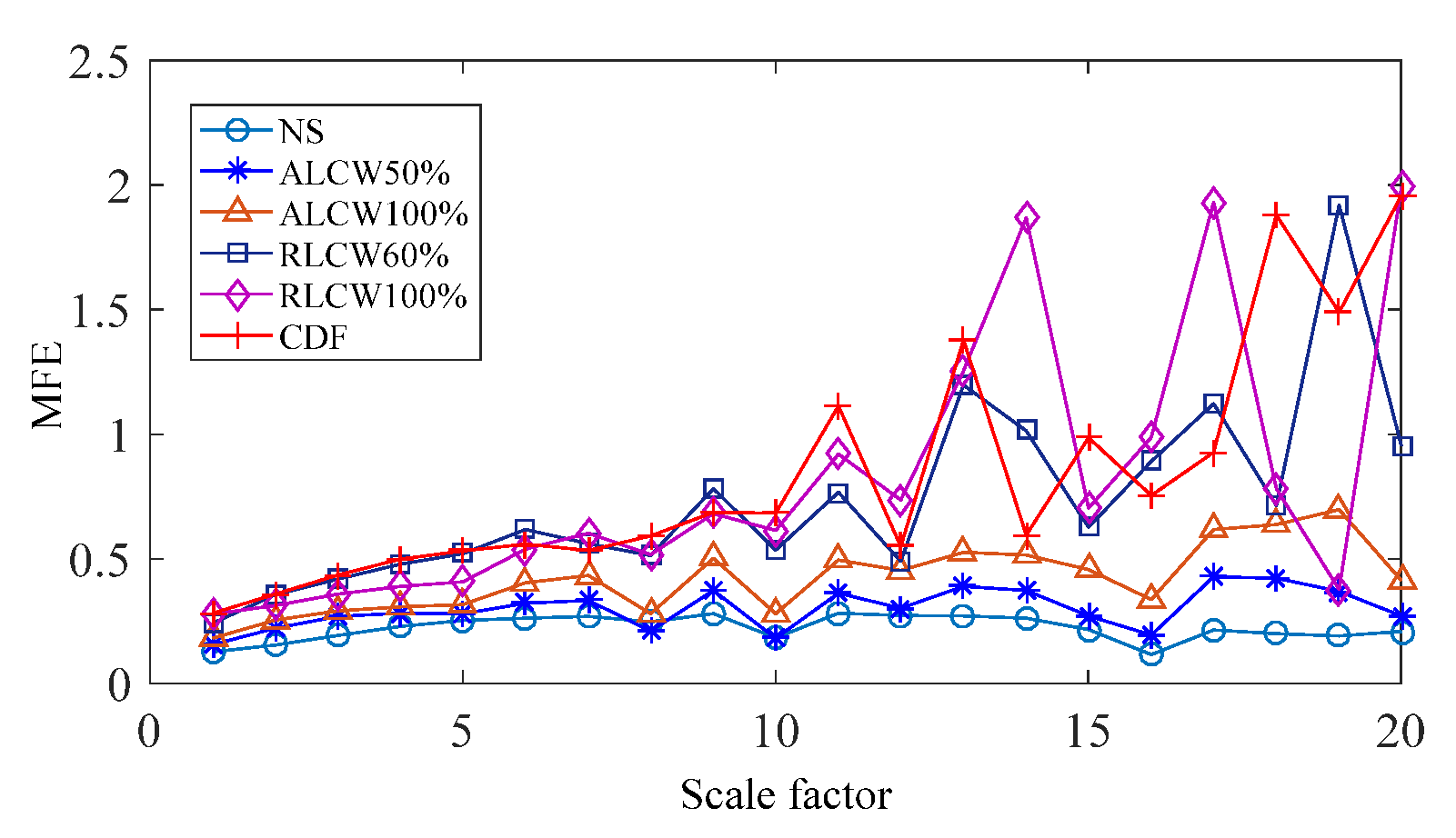
Figure 10 indicates that the MI values corresponding to IMF5 in the six states are all the maximum values, which means that the correlation between IMF5 and the original vibration signal is the strongest. Therefore, we calculate the corresponding MFE value of IMF5 to obtain the feature matrix in all samples. In this case, we set the main parameters of MFE as follows: embedding dimension m = 6, scale factor τ = 20, width of fuzzy function boundary r = 0.1 SD (SD is the standard deviation of IMF5 in different states), and fuzzy function boundary gradient n = 2. Figure 11 shows how the MFE value of IMF5 varies with the scale factor in different states.
Figure 11 reveals that the MFE values of different states are significantly different when the scale factor falls within the range of 1 to 20. Therefore, this paper uses 20 MFE values of IMF5 to construct the feature matrix. As a result, for each state of the HVSR (100 samples), a 100 × 20 feature matrix is generated. We randomly select 70% of each state feature matrix as the training set, and the remaining 30% as the test set. Thus, we obtain a 420 × 20 training subset and a 180 × 20 test subset.
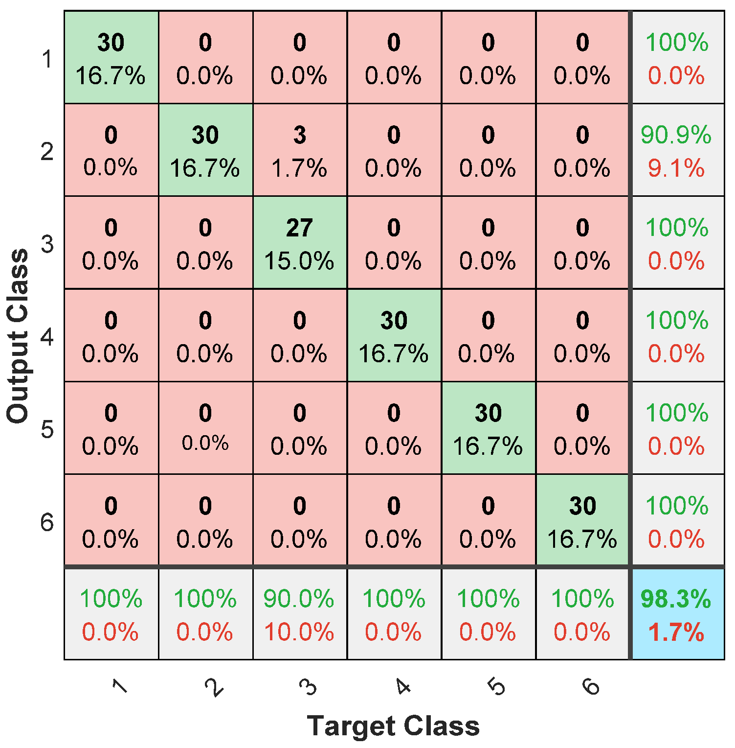
As described in Section 3, this paper further adopts the IGOA-PNN to identify the feature set. We set the population size R of the IGOA to 10 and the maximum number of iterations T to 50. The confusion matrix of the IGOA-PNN recognition results is shown in Figure 12.
As can be seen from Figure 12, the test recognition accuracy of MCPCEEMD-MFE-IGOA-PNN proposed in this paper reaches 98.3%. This means that the proposed method can effectively diagnose different mechanical faults inside the HVSR with high identification accuracy.

4.1.3. Discussion

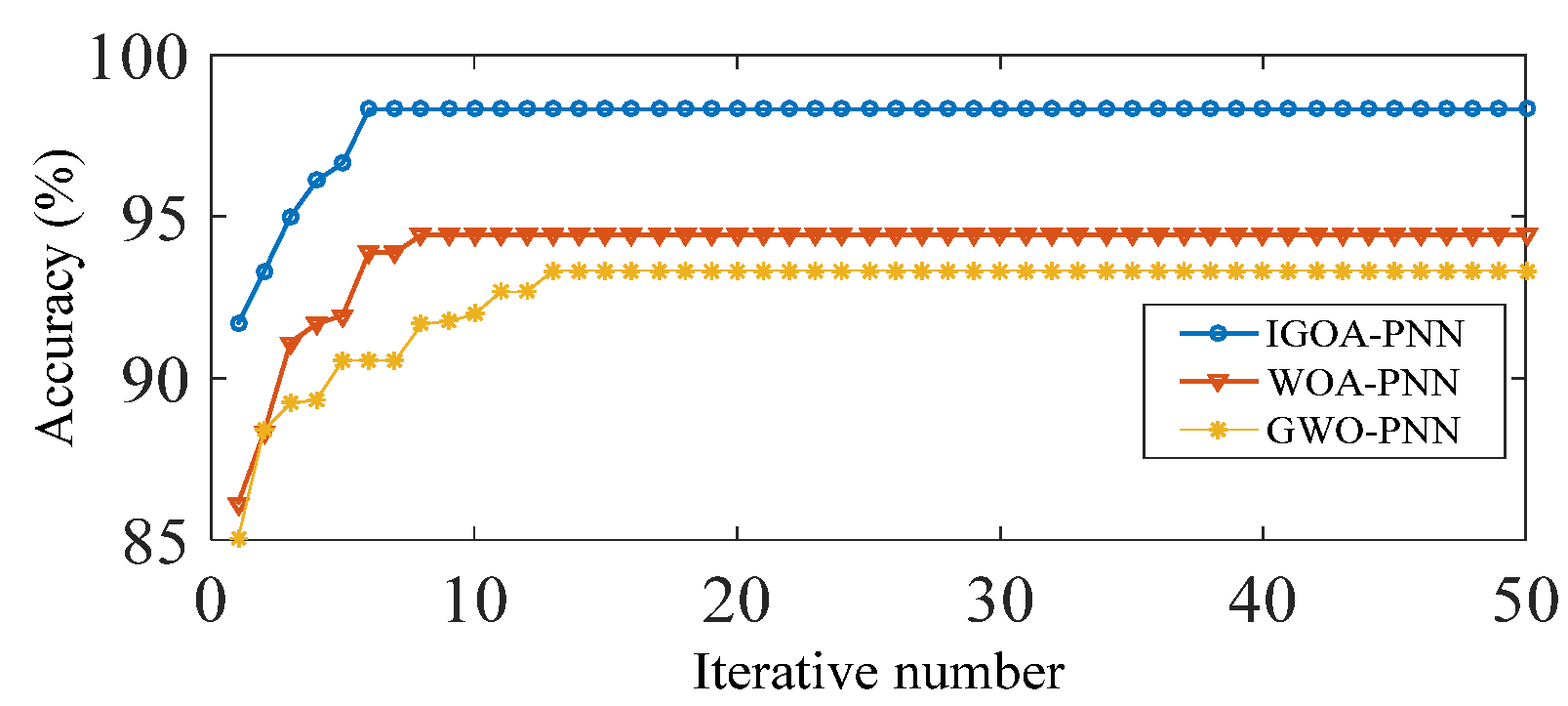
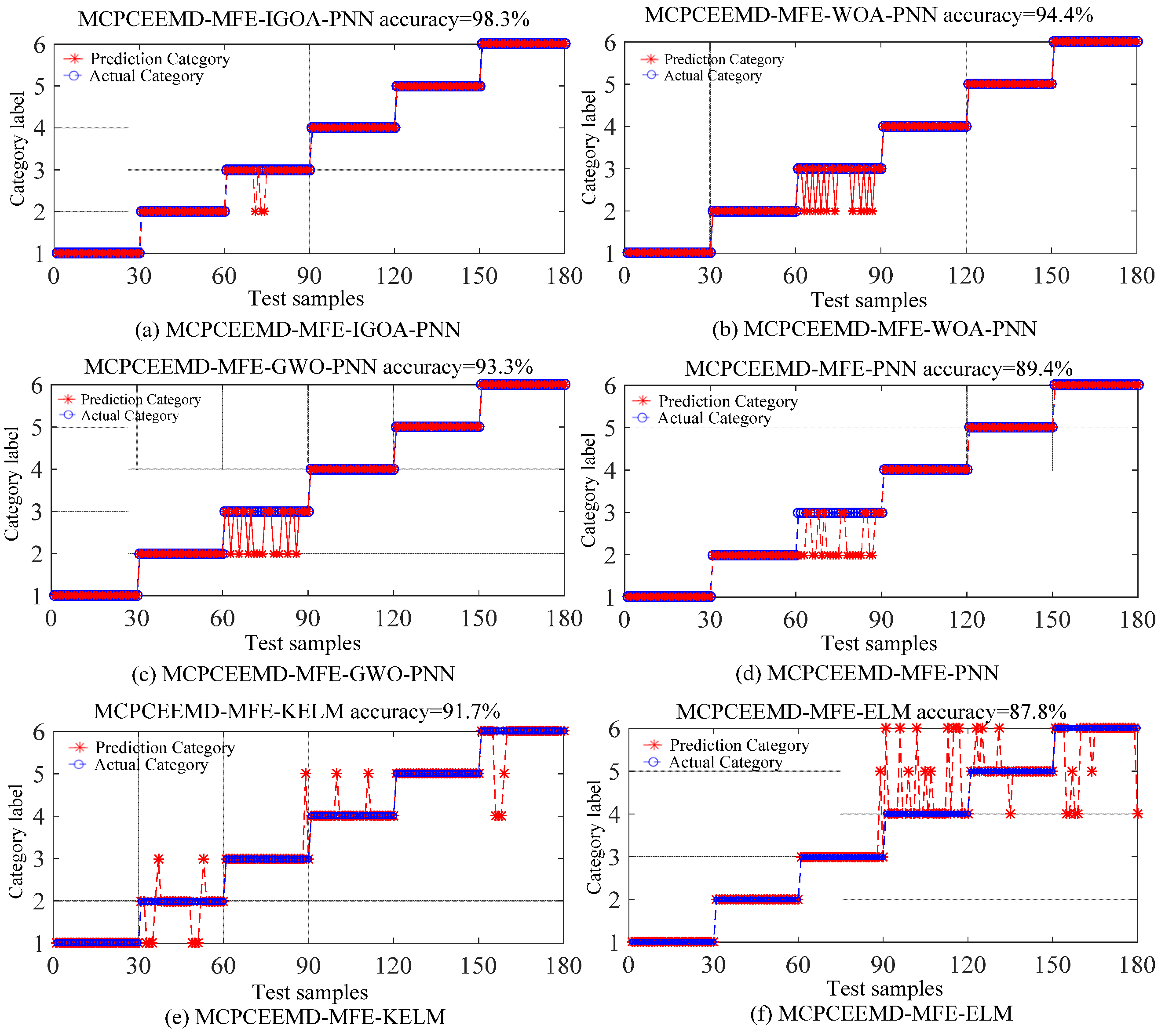
To examine the recognition performance of the proposed IGOA-PNN model, we compare it with the popular whale optimization algorithm optimizing PNN algorithm (WOA-PNN) [35], grey wolf optimization algorithm optimizing PNN algorithm (GWO-PNN) [36], PNN, KELM [37], and ELM [38] classification models. To achieve a fair comparison, we use the parameters with the best experimental results among the five contrastive classification models. Furthermore, the main parameters of the IGOA-PNN, WOA-PNN, and GWO-PNN algorithms are shown in Table 2. In particular, it should be noted that the kernel function of KELM adopts the RBF kernel function, and the hidden layer of ELM is set to 30. The recognition accuracy of different algorithms for optimizing the PNN smoothing factor is shown in Figure 13.
Figure 13 clearly shows the whole process of the recognition accuracy changing with the number of iterations. It can be seen from Figure 13 that the proposed IGOA-PNN model reaches the highest recognition accuracy at the 6th iteration and remains stable. However, the WOA-PNN and the GWO-PNN achieve the highest recognition accuracy at the 8th and 13th iterations, respectively. This means that IGOA is than WOA and GWO in terms of convergence speed. The test recognition results of the proposed method and other comparative models are shown in Figure 14.
Figure 14 demonstrates that the overall recognition accuracy of the proposed model is higher than that of the other three recognition methods. Specifically, the recognition accuracy of the proposed recognition model is 3.9%, 5.0%, 8.9%, 6.6%, and 10.5% higher than that of WOA-PNN (94.4%), GWO-PNN (93.3%), PNN (89.4%), KELM (91.7%), and ELM (87.8%), respectively. This confirms the superiority of the IGOA-PNN model proposed in this paper in solving nonlinear and pattern recognition problems. Therefore, the proposed identification model can provide an excellent diagnosis for HVSR mechanical faults.
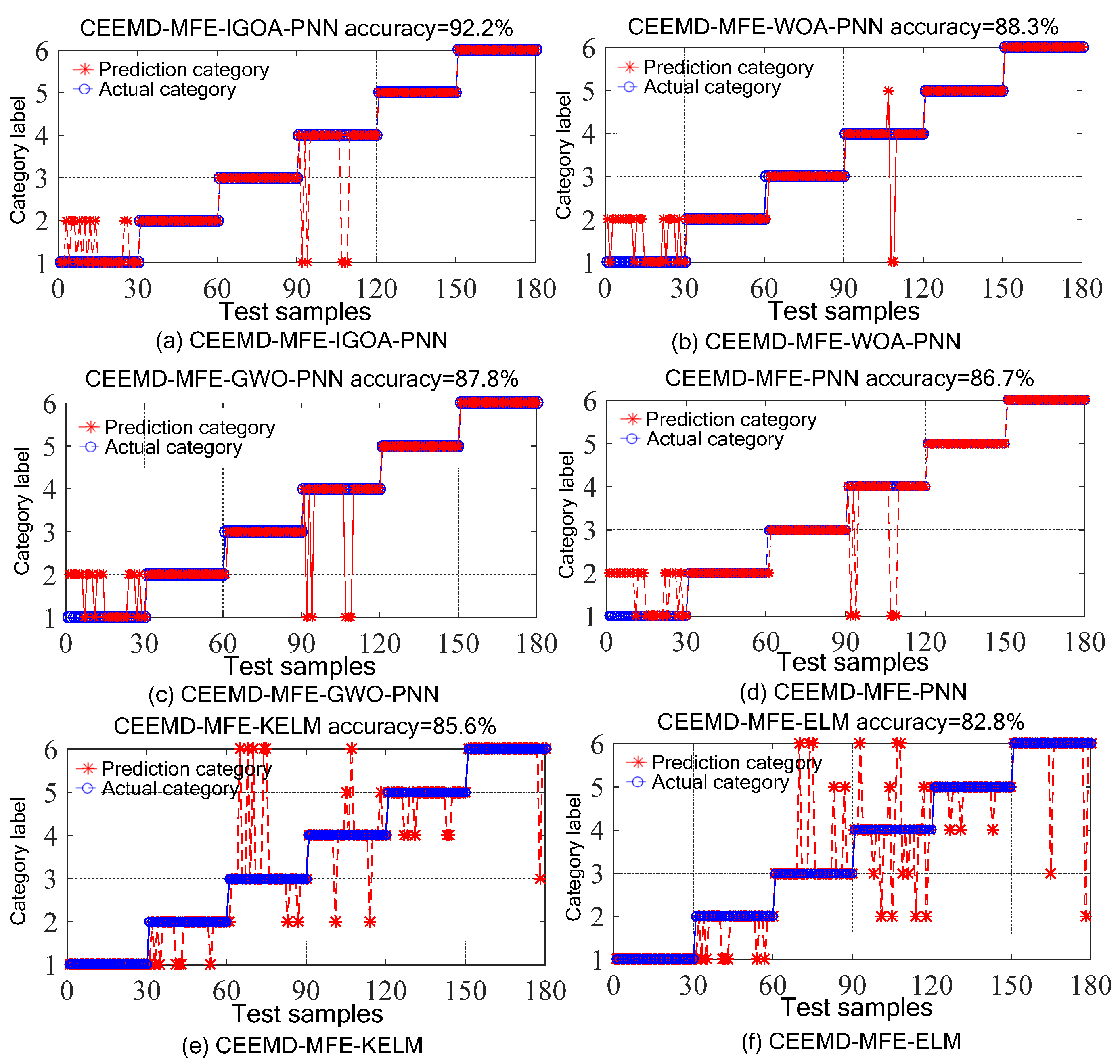
To further demonstrate the superiority of the proposed overall method, we compare and analyze the proposed method with CEEMD-MFE-IGOA-PNN, CEEMD-MFE-WOA-PNN, CEEMD-MFE-GWO-PNN, CEEMD-MFE-PNN, CEEMD-MFE-KELM, and CEEMD-FE-ELM. It should be noted that in the comparison method, except for CEEMD being used to extract the vibration signal, the other calculation steps are the same as those in this paper. The CEEMD white noise logarithm Ne and white noise standard deviation Nstd are set to 50 and 0.2, respectively, which is consistent with our method to guarantee fair comparisons. The recognition results of different methods are shown in Figure 15.
Figure 15 shows that the recognition accuracy of CEEMD-MFE-IGOA-PNN is the highest at 92.2% compared with that of the other methods. This also demonstrates the excellent diagnostic ability of the IGOA-PNN model. However, the accuracy of CEEMD-MFE-IGOA-PNN is 6.1% lower than that of the proposed MCPCEEMD-MFE-IGOA-PNN method. This means that MCPCEEMD improves the shortcomings of CEEMD and improves the decomposition accuracy of HVSR vibration signals. Therefore, the method proposed in this paper has stronger diagnostic performance and higher recognition accuracy for HVSR mechanical faults.

4.2. Case 2: 20 kV HVSR Experimental Verification

4.2.1. Experimental Platform and Data Collection

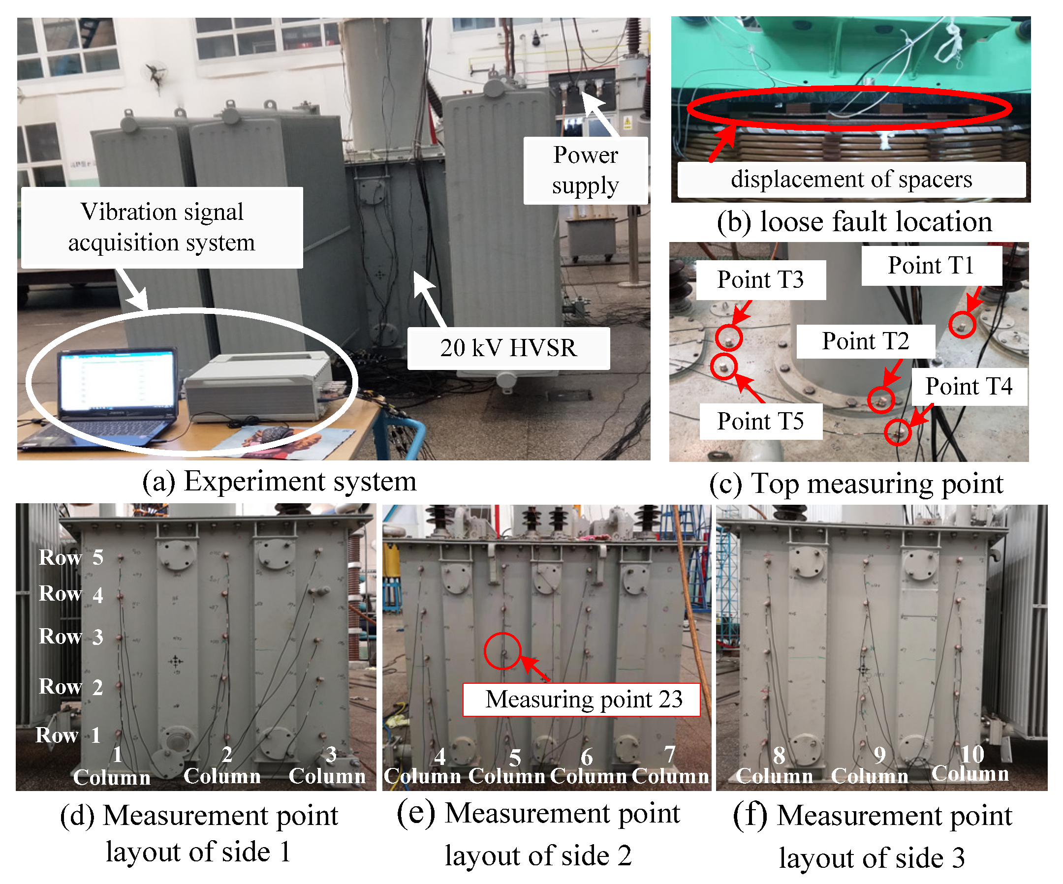
To further test the validity and universality of the proposed method, this paper uses typical fault vibration data collected from a 20 kV HVSR experimental platform for analysis. Figure 16a shows the main components of the experimental platform. The sampling frequency is set to 20 kHz, the sampling time of each group is 10 s, and each state is repeatedly sampled five times. In this case, three typical fault states and the normal state are examined in this study, as shown in Table 3. Figure 16b shows the setting position for a complete loose winding fault. Similar to case 1, the sensor measurement points in this case are also arranged in an array manner, and a total of 55 measurement points are arranged, as shown in Figure 16c–f.
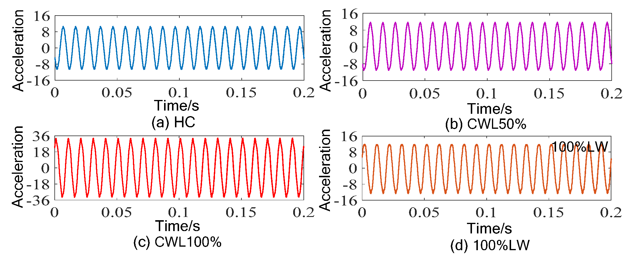
In this case, 4096 sample points are divided into a group. We randomly select 50 groups of each state for feature extraction. Measuring point No. 23 with high vibration intensity in this case is selected for analysis. The location of measuring point No. 23 is shown in Figure 16e. In the four states, the vibration signal waveform of measuring point No. 23 is shown in Figure 17.

4.2.2. Analysis of Results and Discussion

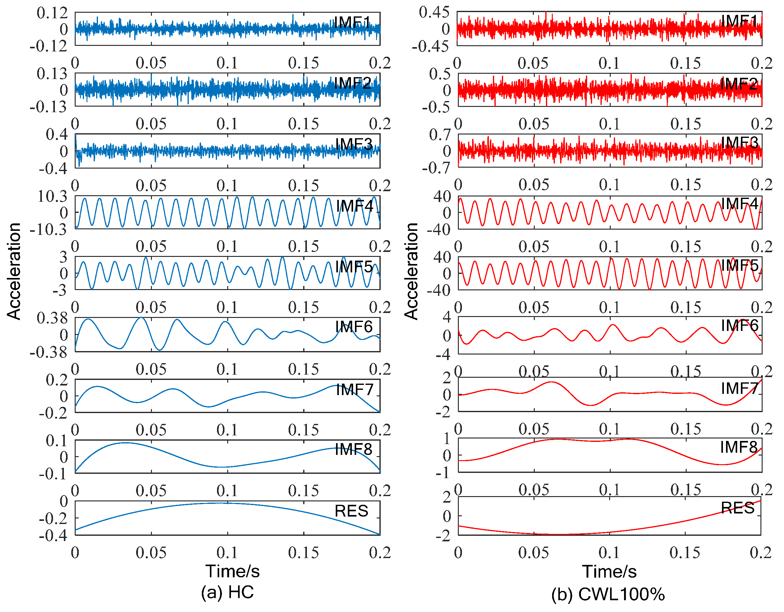
We adopt the proposed MCPCEEMD-MFE-IGOA-PNN for feature extraction and state recognition of vibration signals. It is worth noting that the methods used in this case all use the same parameter settings as Case 1. Figure 18 shows the MCPCEEMD of the vibration signal in both the HC and CWL 100% cases.
The MI theory is used to calculate the MI value of each IMF component obtained by MCPCEEMD. Figure 19 depicts the distribution of MI values for different state IMF components.
Figure 19 demonstrates that the values of IMF4 and IMF5 in each state are relatively close and much higher than those of other IMFs. This implies that IMF4 and IMF5 are strongly correlated with the original vibration signal. Therefore, this case uses the MFE values of IMF4 and IMF5 to construct the feature matrix. Figure 20 presents the MFE values with a scale factor of 20 for IMF4 and IMF5 in different states. Ultimately, the four states (50 samples per state) yield a 400 × 20 feature set. We use 70% of the feature set for training and the remaining 30% for testing.
The IGOA-PNN model is used to classify and identify the feature set. The results of MCPCEEMD-MFE-IGOA-PNN are compared with those of MCPCEEMD-MFE-WOA-PNN, MCPCEEMD-MFE-GWO-PNN, MCPCEEMD-MFE-PNN, MCEPCEEMD-MFE-KELM, and MCPCEEMD-MFE-ELM. It should be noted that the parameters of the comparison method are the optimal parameters obtained from the experiments. The performance comparison results of MCPCEEMD-MFE-IGOA-PNN and other models are shown in Figure 21.
Figure 21 shows that the overall recognition accuracy of MCPCEEMD-MFE-IGOA-PNN is the highest, reaching 99.2%, which is at least 1.7% higher than that of the other comparison methods. This further proves the superiority of the proposed method in fault diagnosis. The high accuracy identification performance of the proposed method is helpful for its practical application in HVSR field maintenance.

5. Conclusions

To identify latent mechanical faults in HVSR more accurately and effectively, this study proposes an intelligent diagnosis method for HVSR mechanical faults based on vibration signals and the MCPCEEMD-MFE-IGOA-PNN method. It is proven that using MCPCEEMD to decompose the vibration signal can further suppress the modal aliasing phenomenon, and the obtained IMFs have better discrimination. When implementing typical mechanical fault identification in HVSR, it should be noted that selecting the IMF with the highest correlation with the original vibration signal is crucial to enhance the accurate diagnosis of the HVSR state. The IMF with the highest correlation is selected based on the MI value in this study. We also optimize the important parameters of PNN by using GOA improved by piecewise inertia weight, which solves the problem that the optimal smoothing factor is difficult to determine. Moreover, the proposed IGOA-PNN model achieves automatic identification of HVSR mechanical faults and higher identification accuracy. The experimental results show that the method proposed in this paper can successfully identify different kinds of latent mechanical faults inside HVSR and can distinguish the fault degree. The comparisons with other advanced recognition methods also demonstrate the superiority of the proposed method. Our next work is to apply the proposed method in the field and continuously optimize the model based on field data. We hope to provide a basis for the on-site maintenance of HVSRs.

Author Contributions

Conceptualization, P.H. and H.M.; methodology, P.H. and H.M.; software, P.H.; validation, H.M. and P.J.; formal analysis, P.H. and H.M.; investigation, H.M. and P.J.; data curation, H.M.; writing—original draft preparation, P.H.; writing—review and editing, P.H. and H.M.; visualization, P.H. and H.M.; supervision, H.M. and P.J.; project administration, P.H.; funding acquisition, H.M. All authors have read and agreed to the published version of the manuscript.

Funding

This work was supported in part by the Fundamental Research Funds for the Central Universities under grant B200203128, in part by the Postgraduate Research & Practice Innovation Program of Jiangsu Province under grant KYCX20_0431, in part by the National Natural Science Foundation of China under grant 51577050, and in part by the Science and Technology Project of State Grid Jiangsu Electric Power Corporation under grant J2018050.

Institutional Review Board Statement

Not applicable.

Informed Consent Statement

Not applicable.

Data Availability Statement

Not applicable.

Acknowledgments

The authors would like to thank Baoding Tianwei Group Co., Ltd., for the 20 kV HVSR experimental platform.

Conflicts of Interest

The authors declare no conflict of interest.

References

  1. Xie, C.; Li, F.; Wang, B.; Fan, Y.; Jing, L.; Chen, W.; Wang, C. Anti-interference adaptive single-phase auto-reclosing schemes based on reactive power characteristics for transmission lines with shunt reactors. Electr. Power Syst. Res. 2019, 170, 176–183. [Google Scholar] [CrossRef]
  2. Xie, C.; Li, F. Adaptive comprehensive auto-reclosing scheme for shunt reactor-compensated transmission lines. IEEE Trans. Power Del. 2020, 35, 2149–2158. [Google Scholar] [CrossRef]
  3. Yang, Q.; Chen, S.; Zeng, X.; Wei, G.; Liu, H.; Chen, T. Suppression measures for overvoltage caused by vacuum circuit breaker switching off 10-kV shunt reactor. IEEE Trans. Power Del. 2020, 35, 540–548. [Google Scholar] [CrossRef]
  4. Velasquez, R.M.A.; Lara, J.V.M. Root cause analysis for shunt reactor failure in 500 kV power system. Eng. Fail. Anal. 2019, 104, 1157–1173. [Google Scholar] [CrossRef]
  5. Das, S.; Sidhu, T.S.; Zadeh, M.R.D.; Zhang, Z.Y. A novel hybrid differential algorithm for turn to turn fault detection in shunt reactors. IEEE Trans. Power Del. 2017, 32, 2537–2545. [Google Scholar] [CrossRef]
  6. Velasquez, R.M.A.; Lara, J.V.M. Methodology for failure analysis in shunt reactor by electromagnetic influence caused by high vibration in overload condition. Eng. Fail. Anal. 2019, 104, 589–608. [Google Scholar] [CrossRef]
  7. Yao, C.; Zhao, Z.; Li, C.; Chen, X.; Zhao, Y.; Zhao, X. Noninvasive method for online detection of internal winding faults of 750 kV EHV shunt reactors. IEEE Trans. Dielectr. Electr. Insul. 2015, 22, 2833–2840. [Google Scholar] [CrossRef]
  8. Zhang, P.; Li, L.; Cheng, Z.; Tian, C.; Han, Y. Study on vibration of iron core of transformer and reactor based on maxwell stress and anisotropic magnetostriction. IEEE Trans. Mag. 2019, 55, 1–5. [Google Scholar] [CrossRef]
  9. Xiao, R.; Zhang, Z.; Wu, Y.; Jiang, P.; Deng, J. Multi-scale information fusion model for feature extraction of converter transformer vibration signal. Measurement 2021, 180, 109555. [Google Scholar] [CrossRef]
  10. Zollanvari, A.; Kunanbayev, K.; Bitaghsir, S.A.; Bagheri, M. Transformer fault prognosis using deep recurrent neural network over vibration signals. IEEE. Trans. Instrum. Meas. 2020, 70, 1–11. [Google Scholar] [CrossRef]
  11. Hou, P.; Ma, H.; Ju, P.; Chen, X.; Zhu, C. A new vibration analysis approach for monitoring the working condition of a high-voltage shunt reactor. IEEE Access 2021, 9, 46487–46504. [Google Scholar] [CrossRef]
  12. Valtierra-Rodriguez, M. Fractal dimension and data mining for detection of short-circuited turns in transformers from vibration signals. Meas. Sci. Technol. 2019, 31, 025902. [Google Scholar] [CrossRef]
  13. Cheng, Q.; Zhao, Z.; Tang, C.; Qian, G.; Islam, S. Diagnostic of transformer winding deformation fault types using continuous wavelet transform of pulse response. Measurement 2019, 140, 197–206. [Google Scholar] [CrossRef]
  14. Zhen, S.; Liu, C.; Liu, X. Research on vibration saltation of the transformer core caused by DC bias of based on empirical mode decomposition. J. Electr. Eng. Technol. 2021, 16, 1185–1192. [Google Scholar] [CrossRef]
  15. Yeh, J.R.; Shieh, J.S. Complementary ensemble empirical mode decomposition: A novel noise enhanced data analysis method. Adv. Adapt. Data Anal. 2010, 2, 135–156. [Google Scholar] [CrossRef]
  16. Cao, C.; Xu, B.; Li, X. Monitoring method on loosened state and deformational fault of transformer winding based on vibration and reactance information. IEEE Access 2020, 8, 215479–215492. [Google Scholar] [CrossRef]
  17. Adler, J.; Parmryd, I. Quantifying colocalization by correlation: The pearson correlation coefficient is superior to the mander’s overlap coefficient. Cytometry A 2010, 77, 733–742. [Google Scholar] [CrossRef]
  18. Yu, X.; Zhang, G.; Yao, W.; Yang, Z. Morphological correlation coefficient and its application in geochemical data analysis. J. Geol. 2019, 43, 103–110. [Google Scholar]
  19. Walczak, Z. Total correlations and mutual information. Phys. Lett. A 2009, 373, 1818–1822. [Google Scholar] [CrossRef] [Green Version]
  20. Ma, Y.; Cheng, J.; Wang, P.; Wang, J.; Yu, Y. Rotating machinery fault diagnosis based on multivariate multiscale fuzzy distribution entropy and fisher score. Measurement 2021, 179, 109495. [Google Scholar] [CrossRef]
  21. Zhang, K.; Cheng, J.; Yang, Y. Roller bearing fault diagnosis based on local mean decomposition and morphological fractal dimension. J. Vib. Shock 2013, 32, 90–94. [Google Scholar]
  22. Noman, K.; Li, Y.; Peng, Z.; Wang, S. Continuous health monitoring of bearing by oscillatory sparsity indices under non stationary time varying speed condition. IEEE Sens. J. 2022, 22, 4452–4462. [Google Scholar] [CrossRef]
  23. Li, C.; Zhou, N.; Liao, J.; Wang, Q. Multiscale multivariate fuzzy entropy-based technique to distinguish transformer magnetizing from fault currents. IET Gener. Transm. Distrib. 2019, 13, 2319–2327. [Google Scholar] [CrossRef]
  24. Yang, X.; Chen, W.; Li, A.; Yang, C.; Xie, Z.; Dong, H. BA-PNN-based methods for power transformer fault diagnosis. Adv. Eng. Inform. 2019, 39, 178–185. [Google Scholar] [CrossRef]
  25. Yan, R.; Liu, Y.; Gao, R. Permutation entropy: A nonlinear statistical measure for status characterization of rotary machines. Mech. Syst. Signal Process. 2012, 29, 474–484. [Google Scholar] [CrossRef]
  26. Zhao, X.; Cheng, J.; Wang, P.; Yang, Y. A rotating machinery fault diagnosis method using composite multiscale fuzzy distribution entropy and minimal error of convex hull approximation. Meas. Sci. Technol. 2020, 32, 025010. [Google Scholar] [CrossRef]
  27. Zheng, D.; Han, B.; Liu, G.; Li, Y.; Yu, H. Cross-Domain intelligent fault diagnosis method of rotating machinery using multi-scale transfer fuzzy entropy. IEEE Access 2021, 9, 95481–95492. [Google Scholar]
  28. Chen, H.; Xiong, Y.; Li, S.; Song, Z.; Hu, Z.; Liu, F. Multi-Sensor Data Driven with PARAFAC-IPSO-PNN for Identification of Mechanical Nonstationary Multi-Fault Mode. Machines 2022, 10, 155. [Google Scholar] [CrossRef]
  29. Saremi, S.; Mirjalili, S.; Lewis, A. Grasshopper Optimisation Algorithm: Theory and application. Adv. Eng. Softw. 2017, 105, 30–47. [Google Scholar] [CrossRef] [Green Version]
  30. Zhang, J.; Zhong, M.; Zhang, J. Detection for weak fault in planetary gear trains based on an improved maximum correlation kurtosis deconvolution. Meas. Sci. Technol. 2019, 31, 025101. [Google Scholar] [CrossRef]
  31. Ye, X.; Hu, Y.; Shen, J.; Feng, R.; Zhai, G. An improved empirical mode decomposition based on adaptive weighted rational quartic spline for rolling bearing fault diagnosis. IEEE Access 2020, 8, 123813–123827. [Google Scholar] [CrossRef]
  32. Yun, K.; Chong, Y.; Song, E.; Yang, L.; Quan, D. A weak fault diagnosis scheme for common rail injector based on MGOA-MOMEDA and improved hierarchical dispersion entropy. Meas. Sci. Technol. 2020, 32, 025012. [Google Scholar] [CrossRef]
  33. Zhu, D.; Wang, L.; Hu, Z.; Yang, S. A Grasshopper Optimization-based fault-tolerant control algorithm for a human occupied submarine with the multi-thruster system. Ocean Eng. 2021, 242, 110101. [Google Scholar] [CrossRef]
  34. Ding, J.; Xiao, D.; Li, X. Gear fault diagnosis based on genetic mutation particle swarm optimization VMD and probabilistic neural network algorithm. IEEE Access 2020, 8, 18456–18474. [Google Scholar] [CrossRef]
  35. Mirjalili, S.; Lewis, A. The Whale Optimization Algorithm. Adv. Eng. Softw. 2016, 95, 51–67. [Google Scholar] [CrossRef]
  36. Mirjalili, S.; Mirjalili, S.M.; Lewis, A. Grey Wolf Optimizer. Adv. Eng. Softw. 2014, 69, 46–61. [Google Scholar] [CrossRef] [Green Version]
  37. Chen, Q.; Wei, H.; Rashid, M.; Cai, Z. Kernel extreme learning machine based hierarchical machine learning for multi-type and concurrent fault diagnosis. Measurement 2021, 184, 109923. [Google Scholar] [CrossRef]
  38. Ding, S.; Zhao, H.; Zhang, Y.; Xu, X.; Nie, R. Extreme learning machine: Algorithm, theory and applications. Artif. Intell. Rev. 2015, 44, 103–115. [Google Scholar] [CrossRef]
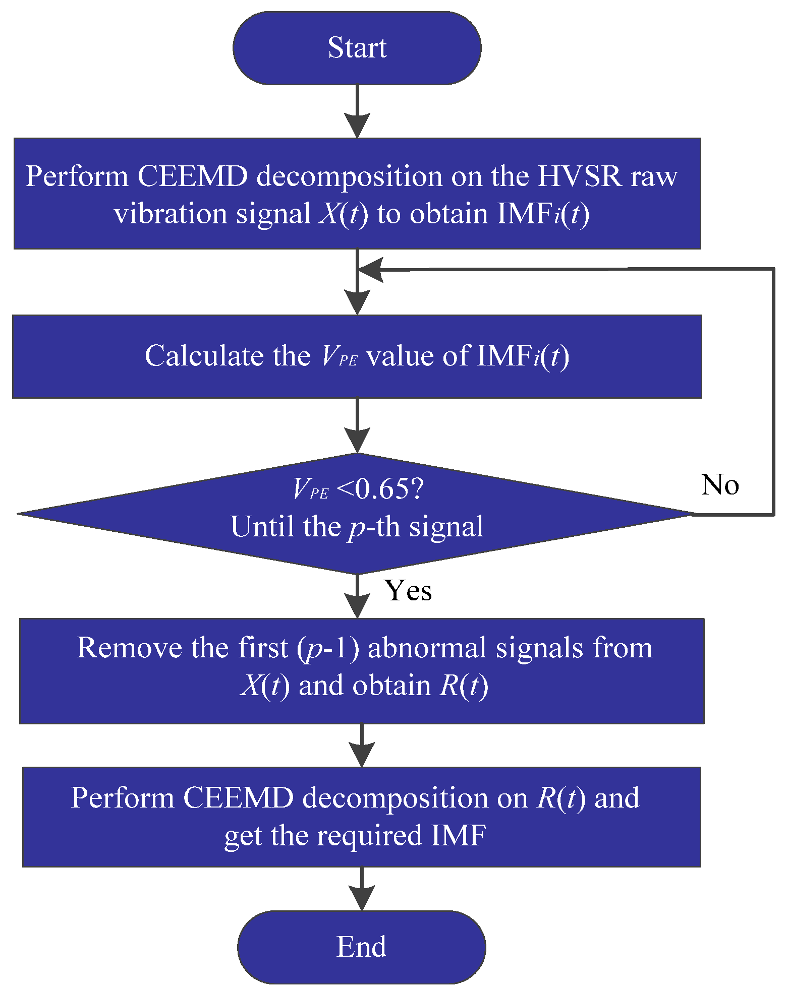
Figure 1. MCPCEEMD flowchart.
Machines 10 00627 g001
Figure 2. PNN topology diagram.
Machines 10 00627 g002
Figure 3. IGOA-PNN flowchart.
Machines 10 00627 g003
Figure 4. The flow chart of MCPCEEMD-MFE-IGOA-PNN.
Machines 10 00627 g004
Figure 5. The working structure of the proposed method.
Machines 10 00627 g005
Figure 6. 10 kV HVSR experimental platform and fault simulation.
Machines 10 00627 g006
Figure 7. Measuring point layout.
Machines 10 00627 g007
Figure 8. Time domain waveform of the vibration signal at measuring point No. 42.
Machines 10 00627 g008
Figure 9. MCPCEEMD calculation results of NS and RLCW100%.
Machines 10 00627 g009
Figure 10. Corresponding MI value curve of the IMF components under different working conditions.
Machines 10 00627 g010
Figure 11. Change curves of the MFE values corresponding to different scale factors in different states.
Machines 10 00627 g011
Figure 12. Confusion matrix of the IGOA-PNN recognition results.
Machines 10 00627 g012
Figure 13. The recognition accuracy curves of different algorithms.
Machines 10 00627 g013
Figure 14. HVSR fault identification results for different models.
Machines 10 00627 g014
Figure 15. Identification results of different methods.
Machines 10 00627 g015
Figure 16. 20 kV HVSR experimental platform.
Machines 10 00627 g016
Figure 17. Vibration signal waveform of measuring point No. 23.
Machines 10 00627 g017
Figure 18. MCPCEEMD calculation results for HC and CWL100%.
Machines 10 00627 g018
Figure 19. MI value curve corresponding to the IMF component in different states.
Machines 10 00627 g019
Figure 20. MFE curves of IMF4 and IMF5.
Machines 10 00627 g020
Figure 21. HVSR mechanical fault identification results.
Machines 10 00627 g021
Table 1. Typical 10 kV HVSR faults.
Category LabelsDifferent States
1Normal status (NS)
250% axial looseness of core winding (ALCW50%)
3100% axial looseness of core winding (ALCW100%)
460% radial looseness of core winding (RLCW60%)
5100% radial looseness of core winding (RLCW100%)
6Component drop failure (CDF)
Table 2. Main parameters of different algorithms.
MethodsParameter Values
IGOA-PNNNumber of species R = 10
Learning factor cmin = 0.0004, cmax = 1
Number of iterations T = 50
WOA-PNNNumber of species R = 10
Weight factor wmin = 0.4, wmax = 0.95
Number of iterations T = 50
GWO-PNNNumber of species R = 10
Number of iterations T = 50
Table 3. 20 kV HVSR fault types.
Category LabelsDifferent States
C1Healthy condition (HC)
C2Core and winding loose 50% (CWL50%)
C3Core and winding loose 100% (CWL100%)
C4100% loose winding (100%LW)
Publisher’s Note: MDPI stays neutral with regard to jurisdictional claims in published maps and institutional affiliations.