Research on Tire/Road Peak Friction Coefficient Estimation Considering Effective Contact Characteristics between Tire and Three-Dimensional Road Surface

Abstract

In the field of transportation, the accurate estimation of tire–road peak friction coefficient (TRPFC) is very important to improve vehicle safety performance and the efficiency of road maintenance. The existing estimation algorithms rarely consider the influence of road roughness and road texture on the estimation results. This paper proposes an estimation method of TRPFC considering the effective contact characteristics between the tire and the three-dimensional road. In the longitudinal and lateral directions of tire–road contact, the model is optimized by incorporating the effective contact area ratio coefficient into the LuGre tire model. The optimized model characterizes the road texture by road power spectrum and establishes the relationship between road texture and tire force. In the vertical direction of tire–road contact, the force transfer between tire and road is represented by a new multi-point contact method. By combining the above models with the normalization method and the unscented Kalman filter (UKF), the timely and accurate estimation of the peak friction coefficient of the tire and the 3D road is realized. Simulation and real vehicle experiments verify the effectiveness of the estimation algorithm.

1. Introduction

At present, the global traffic safety situation is becoming increasingly severe, and the number of traffic accidents is gradually increasing. In 2020, China’s automobile accidents accounted for 64% of the total traffic accidents [1]. The main causes of automobile accidents can be divided into two aspects: improper driving by drivers and the insufficient skid resistance of roads [2,3]. The first aspect can be improved by the continuous improvement of vehicle active safety technology. With the development of intelligent vehicles, vehicle active safety systems are gradually becoming popular in daily life, such as the anti-lock braking system (ABS), traction control system (TCS), and electronic stability system (ESP). They can maximize the fault tolerance rate of the driver’s operation and have become indispensable auxiliary systems to ensure vehicle safety. The second aspect involves road surfacing and routine maintenance. The TRPFC can be used to characterize the skid resistance between the tires and the road surface, which is the basis for the proper operation of active vehicle safety technologies and an indispensable evaluation index for road maintenance [4]. Therefore, the study of the estimation of the coefficient is of great significance for reducing the occurrence of traffic accidents.

In recent years, scholars engaged in research on the estimation of the TRPFC can be broadly divided into two fields, the field of vehicle dynamics and the field of road engineering, which have different emphases. In the field of vehicle dynamics, studies for estimation mostly obtain the TRPFC directly or indirectly by analyzing the vehicle dynamics parameters [5], while in the field of road engineering, studies for measurement are mostly focused on developing measurement methods under specific conditions (certain load, test speed, road texture configuration, etc.). The corresponding empirical models can be established by analyzing experimental data. The predictive calculation of the friction coefficient was performed by the empirical models [6].

Among them, the estimation of the TRPFC in the field of vehicle dynamics can be divided into two categories: test-based and model-based [7]. The test-based approach is based on the direct monitoring of factors related to the TRPFC, which realizes the estimation of the TRPFC. Relevant sensors include the accelerometer on the smart tire [8], ultrasonic sensors [9], magnetometers [10], etc. The method covers a wide range of signals and has a predictive effect, but it is influenced by the environment, expensive, and hard to have a wide range of applications [11,12]. In addition, model-based studies can calculate the change in vehicle dynamics parameters caused by changes in the TRPFC by matching low-cost sensors from which the real-time TRPFC is obtained. The methods can be further divided into four categories: the estimation of the TRPFC based on the slip–slope relationship [13,14,15], fitting based on nonlinear formulas [16,17], fitting based on road state characteristics factors [18], and fitting based on tire models [19,20,21,22]. In summary, the model-based estimation method has a fast reaction velocity, high accuracy, and low hardware cost, but most of the models do not consider the road surface excitation (built on the assumption of a flat road surface) or just simplify it to two-dimensional road surface unevenness. In the actual driving process of the vehicle, the contact between the tire and the road is surface and it is not completely fit, the deviation of model will bring a negative impact to the subsequent work. Therefore, how to reflect the effective contact between the tire and the road in the models is an urgent problem in this field.

In the field of road engineering, it can be broadly divided into two categories: experimental studies and studies on the anti-skid mechanism of road. Since the TRPFC and the road texture structure can directly or indirectly characterize road skid resistance, in experimental studies, corresponding measurement methods have been developed [23,24,25]. In the study of measuring the TRPFC, there are three measuring instruments, the British pendulum tester (BPT) [26], the dynamic friction tester (DFT) [27], and the Wehner/Schulze (W/S) machine [28]. Among them, the BPT has a low cost and simple operation and is convenient to carry, but it is not suitable for high speed. The latter two are suitable for measurement at high speed, but they have high costs. In addition, the test conditions of these three instruments are fixed, there are some differences with the tire–road contact process, they can only be limited to the measurement of the TRPFC under certain working conditions, and the real-time performance cannot be guaranteed [6]. Studies on the measurement of road texture structure make use of the sand spot method [29], the electric sand disk method [30], and the outflow meter method [31]. MTD (mean texture depth) can be obtained and used to characterize the road texture but cannot provide detailed information on the road texture. In summary, most of the studies have focused on the evaluation of road skid resistance under specific conditions using the appropriate measurement devices. There is a lack of deeper studies on the contact friction between the tires and the roads. In addition, the data obtained through measurements are usually a result and cannot form a quantitative expression formula that is relatively widely applicable. On the other hand, in the study of the anti-skid mechanism based on the road surface, scholars have proposed different friction theories and friction components to explain the friction mechanism between the tires and roads, including the following statements. The friction between the tires and roads can be divided into the van der Waals force, the adhesion force, the hysteresis effect within the tire rubber, and the pear chipping effect [32]. The friction between the tires and roads can be obtained by combining the adhesion component and the hysteresis component [33,34]. The friction can be composed of the adhesion component, the hysteresis component, and the pear chipping component [35]. The Persson theoretical friction model focuses more on the hysteresis component [36]. In these studies, hysteresis and adhesion are considered as the main components of friction between tires and roads [37]. In order to obtain a quantitative description of the TRPFC, many scholars introduced contact mechanics into the study of the TRPFC. Hertz derived an expression for contact area pressure based on elastic contact deformation [38], Greenwood and Williamson introduced mathematical statistics into contact theory based on Herz [39], the BGT model (designed by Bush, Gibson, and Thomas) was developed for multi-convex body characteristic contact that involves two different micro-convex body radii of curvature [40], and Persson proposed the concept of the amplification coefficient and associated it with the actual contact area [41]. In summary, the concept of the amplification coefficient can effectively describe the real contact situation between the tires and roads. Compared with the three contact theories above, Persson’s theory takes into account the power spectrum characteristics of the road and the rubber compound modulus and it is more refined and expressive.

In summary, the model-based TRPFC estimation method can accurately estimate the TRPFC in real time based on the vehicle dynamics response caused by the TRPFC, but it is highly dependent on the accuracy of the model. The error of the tire–road contact model in this field is mainly reflected in two aspects: Firstly, in the lateral and longitudinal aspect, the contact area between the tire and the road will vary with the roughness of the road surface. Secondly, in the vertical direction, most of the studies simplify the tire–road contact to point contact rather than surface contact. In addition, in the field of road engineering, the research on the friction mechanism takes more into account the material properties, distribution characteristics, and velocity of the rubber and road. However, it takes less consideration of the vehicle and cannot adapt to the various working conditions encountered in the actual driving process. The real-time performance is difficult to be guaranteed due to the dependence on the collection of experimental data.

Obviously, the advantages and disadvantages of the two fields can be complementary. Therefore, this paper integrates the effective contact area ratio coefficient of tire and the road into the two-dimensional non-uniformly distributed LuGre tire model [42,43], characterizes the road texture by road power spectrum, and establishes the relationship between the road texture and the tire force. For the tire–road vertical contact, which is different from the existing multi-point contact [44], a new multi-point contact is used to replace the single-point contact to describe the vertical contact characteristics. After completing the optimization of the tire–road contact model, the tire model is normalized by the normalization method [45]. Combining with the unscented Kalman filter, the TRPFC is estimated. The simulation was performed with the B-level 3D road excitation input, the real vehicle test was conducted on a dry asphalt road, and both the simulation and test results verified the effectiveness of the method.

The paper is organized as follows: Section 2 describes the overall estimation strategy, Section 3 establishes the vehicle dynamics model, Section 4 introduces the modified tire–road contact model, Section 5 introduces the unscented Kalman filter, Section 6 and Section 7 present the simulation and experimental results, respectively, and Section 8 is the conclusion.

2. Overall Estimation Strategy

The overall estimation flow chart is shown in Figure 1, where $a_x,a_y$ are the longitudinal and lateral accelerations for the vehicle’s center of gravity (CG), respectively, $v_x,v_y$ are the longitudinal and lateral velocities of the CG, respectively, and $\delta ,\gamma ,\omega$ are the front wheel steering angle, yaw rate, and roll angle, respectively. $q$ denotes the road roughness, and $\mathrm{P}\left(\mathrm{q}\right)$ is the effective contact area ratio of the tire/road. The signals (acceleration, velocity, angle, etc.) are output from the real vehicle sensors and CarSim (professional vehicle dynamics simulation software for cars). The multi-point contact model is applied to the vertical dynamic model. The vehicle dynamic model consists of a vertical dynamic model and a side-longitudinal dynamic model. The effective contact area ratio of the tire–road is combined with the two-dimensional non-uniform load distribution LuGre tire model to obtain the modified LuGre tire model. The normalization method is used to normalize the tire model. Based on the above models, the TRPFC is estimated by the UKF.

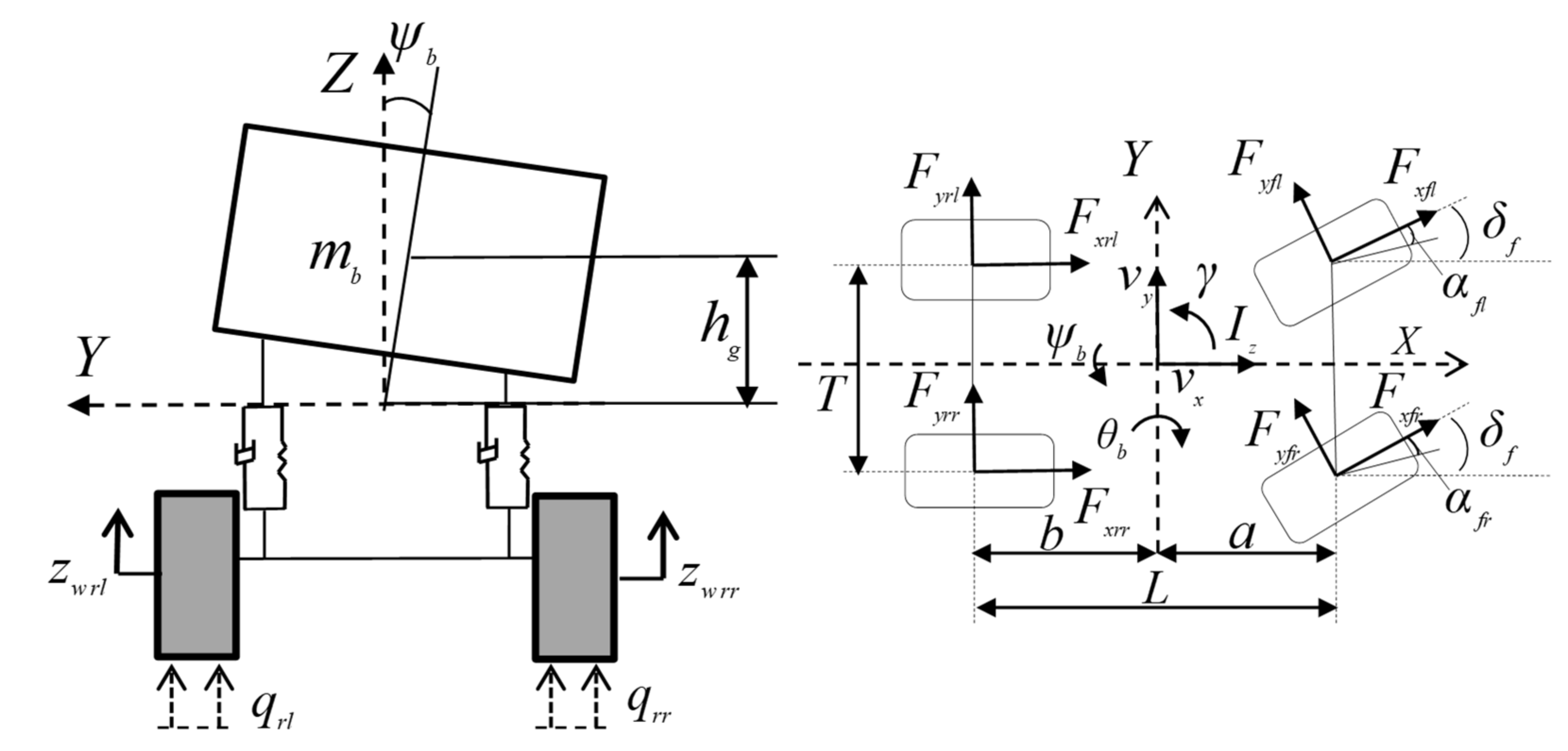
3. Establishment of Vehicle Dynamics Model

The vehicle dynamics model is established, as shown in Figure 2.

The following motion differential equations are established [46,47]:

Equation of longitudinal motion:

$$m_z({\dot{v}}_x-v_y\gamma )+m_b{\dot{z}}_b{\dot{\theta }}_b=F_{xfl}\cos {\delta }_f-F_{yfl}\sin {\delta }_f+F_{xfr}\cos {\delta }_f-F_{yfr}\sin {\delta }_f+F_{xrl}+F_{xrr}$$

(1)

Equation of lateral motion:

$$m_z({\dot{v}}_y+v_x\gamma )-m_b{\dot{z}}_b{\dot{\psi }}_b-m_b{h}_g{\ddot{\psi }}_b=F_{xfl}\sin {\delta }_f+F_{yfl}\cos {\delta }_f+F_{xfr}\sin {\delta }_f+F_{yfr}\cos {\delta }_f+F_{yrl}+F_{yrr}$$

(2)

Equation of yaw motion:

$$\dot{\gamma }{I}_z+I_{xz}{\ddot{\psi }}_b=a(F_{xfl}\sin {\delta }_f+F_{yfl}\cos {\delta }_f+F_{xfr}\sin {\delta }_f+F_{yfr}\cos {\delta }_f)+\frac{T}{2}(F_{xrr}+F_{xfr}\cos {\delta }_f-F_{yfr}\sin {\delta }_f)-\frac{T}{2}(F_{xfl}\cos {\delta }_f-F_{yfl}\sin {\delta }_f+F_{xrl})-(F_{yrl}+F_{yrr})b$$

(3)

The load on each wheel can be expressed as:

$$F_{zfl}=\frac{b}{2L}{m}_{z}g-\frac{b{h}_g}{LT}{m}_b{a}_y-\frac{m_b{a}_x{h}_g}{2L}+K_{\psi }{\psi }_b+K_w(z_{wfl}-q_{fl})$$

(4)

$$F_{zfr}=\frac{b}{2L}{m}_{z}g+\frac{b{h}_g}{LT}{m}_b{a}_y-\frac{m_b{a}_x{h}_g}{2L}+K_{\psi }{\psi }_b+K_w(z_{wfr}-q_{fr})$$

(5)

$$F_{zrl}=\frac{a}{2L}{m}_{z}g-\frac{a{h}_g}{LT}{m}_b{a}_y+\frac{m_b{a}_x{h}_g}{2L}+K_{\psi }{\psi }_b+K_w(z_{wrl}-q_{rl})$$

(6)

$$F_{zrr}=\frac{a}{2L}{m}_{z}g+\frac{a{h}_g}{LT}{m}_b{a}_y+\frac{m_b{a}_x{h}_g}{2L}+K_{\psi }{\psi }_b+K_w(z_{wrr}-q_{rr})$$

(7)

where $F_{xfl},F_{xfr},F_{xrl},F_{xrr},F_{yfl},F_{yfr},F_{yrl},F_{yrr}$ are the longitudinal tire force and the lateral tire force of four wheels, respectively. $v_x,v_y$ are the longitudinal and lateral velocities for the CG, respectively. $\gamma ,{\psi }_b,{\delta }_f$, ${\theta }_b$ are the yaw rate, roll angle, front wheel steering angle, and pitch angle, respectively. g is $9.8m/s^2$, and $a_x,a_y$ are the longitudinal and lateral accelerations of the CG respectively. $I_{xz}$ is the product of inertia for the vehicle in axles X and Z. ${\alpha }_{fl}$, ${\alpha }_{fr}$ are the slip angles for front wheels, respectively. $q_i(i=fl,fr,rl,rr)$ denote the road roughness for the four wheels. $z_w{}_i(i=fl,fr,rl,rr)$ denote the vertical displacement for the centroid of the four wheels, respectively. The main parameters of vehicle dynamics model are shown in

Table 1. Main parameters of vehicle.

Symbol	Value and Unit	Parameter Name
mz	880 kg	Total vehicle mass
mb	788 kg	Sprung mass
L	2.040 m	Wheel base
a	1.145 m	Distance from centroid to front axle
b	0.895 m	Distance from centroid to rear axle
hg	0.54 m	Centroid height
T	1.3 m	Wheel track width
Iz	832.3 kg · m2	Moment of inertia about the z-axis
Kψ	25,041 N/rad	Tire cornering stiffness
$K_b$	$19.6 \mathrm{kN}/\mathrm{m}$	Stiffness coefficient of suspension system
$c_b$	$1450 \mathrm{N}\cdot \mathrm{s}/\mathrm{m}$	Damping Constant of Suspension Buffer
$K_w$	$250 \mathrm{kN}/\mathrm{m}$	Tire stiffness coefficient
$C_w$	$375 \mathrm{N}\cdot \mathrm{s}/\mathrm{m}$	Tire damping coefficient

, which can be used to describe the vehicle in the test.

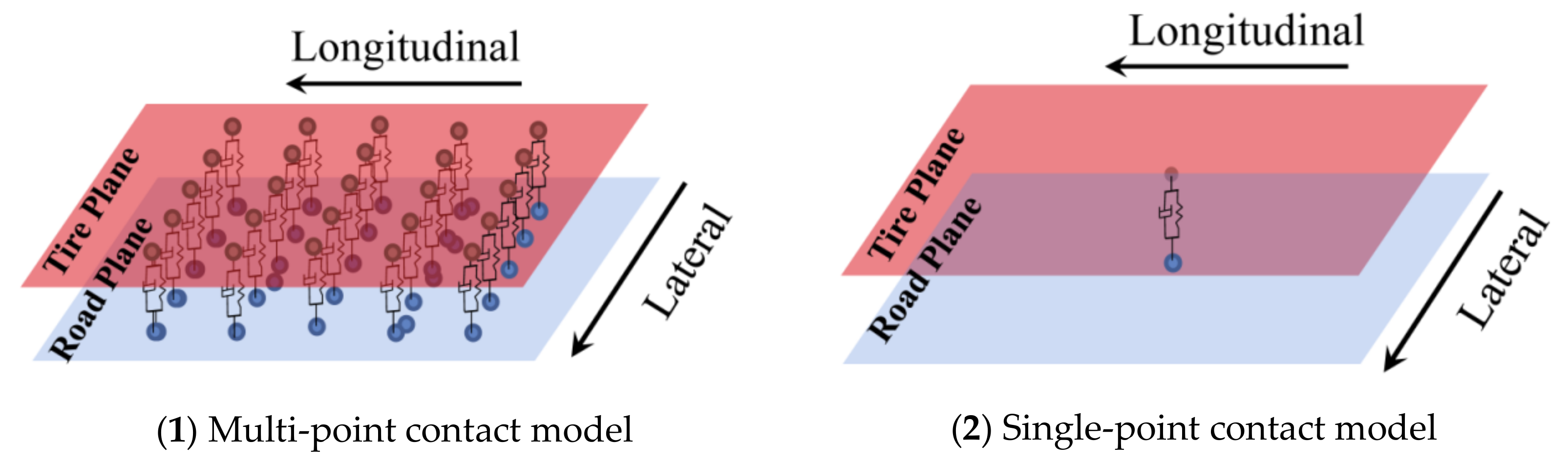
4. Modified Tire/Road Contact Model

4.1. Vertical Dynamics Model

The construction of the vertical dynamics model is shown in Figure 3 and Figure 4. Figure 3(1) shows the multi-point contact model. The tire–road contact part is discretized into 25 contact elements, and the three-dimensional road surface is discretized into 25 function points for road roughnesses, corresponding to the 25 contact elements respectively. After the three-dimensional road vertical excitation is processed by the multi-point contact model between the tires and the roads, the contact point between the tire and the suspension is equivalent to a concentrated point to study.

The multi-point contact model has been applied to a quarter suspension model, as Figure 4 shows.

The equation of vertical motion can be expressed as:

$$\left\{\begin{array}{c}{m}_{wq}{\ddot{z}}_{wi}+C_b({\dot{z}}_{wi}-{\dot{z}}_{bi})+K_b(z_{wi}-z_{bi})+{\displaystyle \sum _{i=1}^n{c}_{wi}}({\dot{z}}_{wi}-{\dot{q}}_i)+{\displaystyle \sum _{i=1}^n{k}_{wi}}(z_{wi}-q_i)=0\\ m_{bq}{\ddot{z}}_{bi}+C_b({\dot{z}}_{bi}-{\dot{z}}_{wi})+K_b(z_{bi}-z_{wi})=0\end{array}\right.$$

(8)

$$\left\{\begin{array}{l}{k}_{wi}=\frac{K_w}{n}\\ c_{wi}=\frac{C_w}{n}\end{array}\right.$$

(9)

where $k_{wi}$ is the tire distribution stiffness coefficient, $c_{wi}$ is the tire distribution damping coefficient, $m_{wq}$ is the unsprung mass,$m_{bq}$ is the sprung mass, $z_w{}_i(i=fl,fr,rl,rr)$ denote the vertical displacement for the centroid of the four wheels, respectively, $z_b{}_i(i=fl,fr,rl,rr)$ denote the vertical displacement for the sprung mass, and n is the number of discrete points.

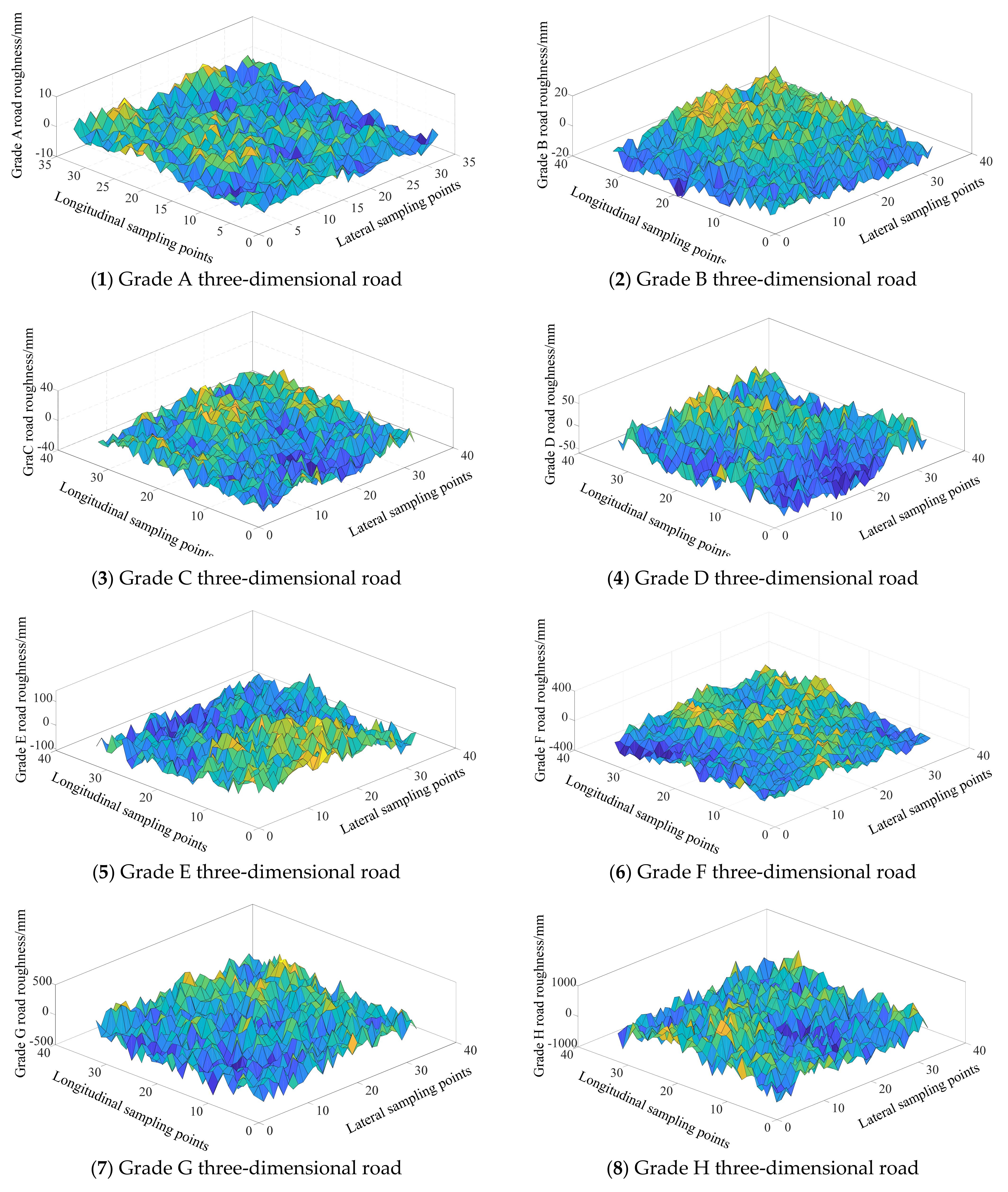
4.2. Construction of 3D Road

Vertical road excitation has a great influence on the dynamic performance of vehicles. Establishing an accurate road model is very important to improve simulation accuracy. Therefore, the 3D road was reconstructed according to the fractal theory [44], as shown in Figure 5, which was used to act as a 3D road excitation during the simulation.

4.3. Modified LuGre Tire Model

To consider the effective contact characteristics of the tire/road in the tire model, it is known from Persson’s theory [41] that the effective contact area ratio of the tire/road can be expressed as:

$$P(q)\approx {(1+{(\pi G(q))}^{\frac{3}{2}})}^{-\raisebox{1ex}{$1$}\!\left/ \!\raisebox{-1ex}{$3$}\right.}$$

(10)

$$G(q)=\frac{1}{8}{\displaystyle \underset{q_L}{\overset{q}{\int }}{q}^{3}C(q)dq}{\displaystyle \underset{0}{\overset{2\pi }{\int }}d}\phi {\left|\frac{E(qv\cos \phi )}{(1-{\gamma }^2){\sigma }_0}\right|}^2$$

(11)

where $C(q)$ is the road power spectral density function, which can be expressed as [48]:

$$C(n\text{'})=C(n_0){(\frac{n\text{'}}{n_0})}^{-W}$$

(12)

where $C(n_0)$ is the road power spectral density value at the reference spatial frequency, which varies on different roads [48], $n^{\prime }$ is the spatial frequency, $n_0$ is the reference spatial frequency, $C(n_0)$ is the road power spectral density value under the reference spatial frequency, and W is the frequency index.

Based on the LuGre tire model in reference [42,43], combining with Equations (10) and (11), the modified LuGre tire model can be expressed as:

$$F_{x,y}=P(q)\cdot [F_z\cdot ({\sigma }_{0x,y}{C}_{1x,y}+{\sigma }_{2x,y}{v}_{rx,y})-\frac{F_z}{2}\cdot A_1{\sigma }_{0x,y}{C}_{1x,y}{I}_{F_{x,y}}^{(n_1)}]$$

(13)

$$M_z=P(q)\cdot a{F}_z\cdot [\frac{1}{2}{A}_1{\sigma }_{0y}{C}_{1y}{I}_{M_z}^{(n_1)}-({\sigma }_{0y}{C}_{1y}+{\sigma }_{2y}{v}_{ry})\cdot \frac{{\Delta }_1}{a}]+b{F}_z\cdot \frac{{\Delta }_2}{b}[\frac{1}{4}{A}_1{\sigma }_{0x}{C}_{1x}{I}_{F_x}^{(n_1)}-({\sigma }_{0x}{C}_{1x}+{\sigma }_{2x}{v}_{rx})]$$

(14)

$$I_{F_{x,y}}^{(n_1)}=I_{1x,y}-B_1{I}_{2x,y}+({\lambda }_1-1)I_{(2n_1+1)x,y}-B_1({\lambda }_1-1)I_{(2n_1+2)x,y}-{\lambda }_1{I}_{(4n_1+1)x,y}+B_1{I}_{(4n_1+2)x,y}$$

(15)

$$I_{M_z}^{(n_1)}=I_{2y}-B_1{I}_{3y}+({\lambda }_1-1)I_{(2n_1+2)y}-B_1({\lambda }_1-1)I_{(2n_1+3)y}-{\lambda }_1{I}_{(4n_1+2)y}+B_1{I}_{(4n_1+3)y}$$

(16)

$$I_{ix,y}=-\frac{C_{2x,y}}{a}[\exp (-2a/C_{2x,y})+{(-1)}^{i-1}-i{I}_{(i-1)x,y}](i=1,2)$$

(17)

$$C_{1x,y}=\frac{v_{rx,y}\theta g_{x,y}(v_{rx,y})}{\left|v_{rx,y}\right|{\sigma }_{0x,y}}$$

(18)

$$C_{2x,y}=\left|\frac{\omega r}{v_{rx,y}}\right|\cdot \frac{\theta g_{x,y}(v_{rx,y})}{{\sigma }_{0x,y}}$$

(19)

$$g(v_r)={\mu }_c+({\mu }_s-{\mu }_c)\exp (-{\left|v_r/v_s\right|}^{a_s})$$

(20)

$$A_1=\frac{(2n_1+1)(4n_1+1)}{2n_1(4n_1+1+{\lambda }_1)}$$

(21)

$$B_1=-\frac{3(2n_1+3)(4n_1+3)(4n_1+1+{\lambda }_1)(}{(2n_1+1)(4n_1+1)(4n_1+3+3{\lambda }_1)}\cdot \frac{{\Delta }_1}{a}$$

(22)

The tire slip angle can be expressed as:

$$\alpha =\delta -{\tan }^{-1}(\frac{v_{ty}}{\left|v_{tx}\right|})$$

(23)

where $v_{tx}$ is the longitudinal wheel speed and $v_{ty}$ is the lateral wheel speed.

The slip ratio can be expressed as:

$$s_x=\left\{\begin{array}{l}\frac{\omega r\cdot \cos \alpha -v_w}{v_w} , \mathrm{if} \mathrm{braking}\\ \frac{\omega r\cdot \cos \alpha -v_w}{\omega r\cdot \cos \alpha } , \mathrm{if} \mathrm{driving} \end{array}\right.$$

(24)

$$s_y=\left\{\begin{array}{l}\frac{\omega r\cdot \sin \alpha }{v_w} , \mathrm{if} \mathrm{braking}\\ \tan \alpha , \mathrm{if} \mathrm{driving}\end{array}\right.$$

(25)

$$s_{\mathrm{R}}=\sqrt{s_x^2+s_y^2}\le 1$$

(26)

The other parameters of the tire model can be found in references [42,43].

4.4. Tire Model Normalization

According to the normalization method [45], there are:

$$F_x={\mu }_{R\max g}{F}_x^0$$

(27)

$$F_{{}_x}^0=\frac{P(q)\cdot s_x}{{\mu }_{R\max h}\cdot s_R}\left(F_z\cdot ({\sigma }_{0x}{C}_{1x}+{\sigma }_{2x}{v}_{rx})-\frac{F_z}{2}\cdot A_1{\sigma }_{0x}{C}_{1x}{I}_{F_x}^{(n_1)}\right)$$

(28)

$$F_y={\mu }_{R\max g}{F}_y^0$$

(29)

$$F_{{}_y}^0=\frac{P(q)\cdot s_y}{{\mu }_{R\max h}\cdot s_R}\left(F_z\cdot ({\sigma }_{0y}{C}_{1y}+{\sigma }_{2y}{v}_{ry})-\frac{F_z}{2}\cdot A_1{\sigma }_{0y}{C}_{1y}{I}_{F_y}^{(n_1)}\right)$$

(30)

where ${\mu }_{R\max h}$ is the peak friction coefficient of the adjacent road [45] and $F_x^0$, $F_y^0$ are the longitudinal and lateral normalized forces, respectively, independent of the peak friction coefficient to be identified.

4.5. Establishment of System Equations

In order to estimate the peak friction coefficient of the tire/road, according to Equations (1)–(3), (27), and (29), there are:

$${\dot{v}}_x-v_y\gamma +\frac{m_b}{m_z}({\dot{z}}_b{\dot{\theta }}_b)={\mu }_{fl}(\frac{F_{{}_{xfl}}^0\cos {\delta }_f}{m_z}-\frac{F_{{}_{yfl}}^0\sin {\delta }_f}{m_z}(+{\mu }_{rl}\frac{F_{{}_{xrl}}^0}{m_z}+{\mu }_{fr}(\frac{F_{{}_{xfr}}^0\cos {\delta }_f}{m_z}-\frac{F_{{}_{yfr}}^0\sin {\delta }_f}{m_z}(+{\mu }_{rr}\frac{F_{{}_{xrr}}^0}{m_z}$$

(31)

$${\dot{v}}_y+v_x\gamma -\frac{m_b}{m_z}({\dot{z}}_b\dot{\psi }+h_g{\ddot{\psi }}_b)={\mu }_{rl}\frac{F_{{}_{yrl}}^0}{m_z}+{\mu }_{rr}\frac{F_{{}_{yrr}}^0}{m_z}+{\mu }_{fl}(\frac{F_{{}_{xfl}}^0\sin {\delta }_f}{m_z}+\frac{F_{{}_{yfl}}^0\cos {\delta }_f}{m_z}(+{\mu }_{fr}(\frac{F_{{}_{xfr}}^0\sin {\delta }_f}{m_z}+\frac{F_{{}_{yfr}}^0\cos {\delta }_f}{m_z}($$

(32)

$$\begin{array}{l}\dot{\gamma }+\frac{I_{xz}}{I_z}{\ddot{\psi }}_b={\mu }_{fl}(\frac{a}{I_z}{F}_{{}_{xfl}}^0\sin {\delta }_f-\frac{T}{2I_z}{F}_{{}_{xfl}}^0\cos {\delta }_f+\frac{a}{I_z}{F}_{{}_{yfl}}^0\cos {\delta }_f+\frac{T}{2I_z}{F}_{{}_{yfl}}^0\sin {\delta }_f)+{\mu }_{fr}(\frac{a}{I_z}{F}_{{}_{xfr}}^0\sin {\delta }_f+\frac{T}{2I_z}{F}_{{}_{xfr}}^0\cos {\delta }_f+\frac{a}{I_z}{F}_{{}_{yfr}}^0\cos {\delta }_f-\frac{T}{2I_z}{F}_{{}_{yfr}}^0\sin {\delta }_f)\\ -{\mu }_{rl}(\frac{T}{2I_z}{F}_{{}_{xrl}}^0+\frac{b}{I_z}{F}_{{}_{yrl}}^0(+{\mu }_{rr}(\frac{T}{2I_z}{F}_{{}_{xrr}}^0-\frac{b}{I_z}{F}_{{}_{yrr}}^0(\end{array}$$

(33)

From the above Equations (31)–(33), the equation of state is obtained as follows:

$$\left(\begin{array}{c}{\mu }_{fl}(n+1)\\ {\mu }_{fr}(n+1)\\ {\mu }_{rl}(n+1)\\ {\mu }_{rr}(n+1)\end{array}\right)=\left(\begin{array}{cccc}1& 0& 0& 0\\ 0& 1& 0& 0\\ 0& 0& 1& 0\\ 0& 0& 0& 1\end{array}\right)\left(\begin{array}{l}{\mu }_{fl}(n)\\ {\mu }_{fr}(n)\\ {\mu }_{rl}(n)\\ {\mu }_{rr}(n)\end{array}\right)+w(t)$$

(34)

The measurement equation can be expressed as follows:

$$\left(\begin{array}{c}{\dot{v}}_x-v_y\gamma +\frac{m_b}{m_z}({\dot{z}}_b{\dot{\theta }}_b)\\ {\dot{v}}_y+v_x\gamma -\frac{m_b}{m_z}({\dot{z}}_b\dot{\psi }+h_g{\ddot{\psi }}_b)\\ \dot{\gamma }+\frac{I_{xz}}{I_z}{\ddot{\psi }}_b\end{array}\right)=\left(\begin{array}{cccc}H(1,1)& H(1,2)& H(1,3)& H(1,4)\\ H(2,1)& H(2,2)& H(2,3)& H(2,4)\\ H(3,1)& H(3,2)& H(3,3)& H(3,4)\end{array}\right)\left(\begin{array}{l}{\mu }_{fl}\\ {\mu }_{fr}\\ {\mu }_{rl}\\ {\mu }_{rr}\end{array}\right)+v(t)$$

(35)

$$\left\{\begin{array}{cc}\hfill & H(1,1)=\frac{F_{{}_{xfl}}^{0}cos{\delta }_f}{m_z}-\frac{F_{{}_{yfl}}^{0}sin{\delta }_f}{m_z}\hfill \\ \hfill & H(1,2)=\frac{F_{{}_{xfr}}^{0}cos{\delta }_f}{m_z}-\frac{F_{{}_{yfr}}^{0}sin{\delta }_f}{m_z}\hfill \\ \hfill & H(1,3)=\frac{F_{{}_{xrl}}^0}{m_z},H(1,4)=\frac{F_{{}_{xrr}}^0}{m_z}\hfill \\ \hfill & H(2,1)=\frac{F_{{}_{xfl}}^{0}sin{\delta }_f}{m_z}+\frac{F_{{}_{yfl}}^{0}cos{\delta }_f}{m_z}\hfill \\ \hfill & H(2,2)=\frac{F_{{}_{xfr}}^{0}sin{\delta }_f}{m_z}+\frac{F_{{}_{yfr}}^{0}cos{\delta }_f}{m_z}\hfill \\ \hfill & H(2,3)=\frac{F_{{}_{yrl}}^0}{m_z},H(2,4)=\frac{F_{{}_{yrr}}^0}{m_z}\hfill \\ \hfill & H(3,1)=\frac{a}{I_z}{F}_{{}_{xfl}}^{0}sin{\delta }_f-\frac{T}{2I_z}{F}_{{}_{xfl}}^{0}cos{\delta }_f+\frac{a}{I_z}{F}_{{}_{yfl}}^{0}cos{\delta }_f+\frac{T}{2I_z}{F}_{{}_{yfl}}^{0}sin{\delta }_f\hfill \\ \hfill & H(3,2)=\frac{a}{I_z}{F}_{{}_{xfr}}^{0}sin{\delta }_f+\frac{T}{2I_z}{F}_{{}_{xfr}}^{0}cos{\delta }_f+\frac{a}{I_z}{F}_{{}_{yfr}}^{0}cos{\delta }_f-\frac{T}{2I_z}{F}_{{}_{yfr}}^{0}sin{\delta }_f\hfill \\ \hfill & H(3,3)=-\frac{T}{2I_z}{F}_{{}_{xrl}}^0-\frac{b}{I_z}{F}_{{}_{yrl}}^0\hfill \\ \hfill & H(3,4)=\frac{T}{2I_z}{F}_{{}_{xrr}}^0-\frac{b}{I_z}{F}_{{}_{yrr}}^0\hfill \end{array}\right.$$

(36)

where ${\mu }_{ij}(ij=fl,fr,rl,rr)$ represent the peak friction coefficients between the four tires and surface of the target road, respectively, and the random variables $w(t)$ and $v(t)$ are process noise and measurement noise, respectively.

5. Unscented Kalman Filter

The estimation flow of the UKF [10] can be expressed as shown in Figure 6. The initial values in the filtering process are the measurement noise covariance, $R=0.02\cdot I_{3\times 3}$, the process noise covariance, $Q=0.01\cdot I_{4\times 4}$, and the corresponding covariance matrix, $P_0=0.1\cdot I_{4\times 4}$.

6. Simulation Verification Analysis

Two operating conditions that included the straight-line braking condition and the combined turning and braking condition were simulated by CarSim and Matlab/Simulink. By replacing the internal tire model of CarSim with the modified LuGre tire model and replacing the tire-suspension part, a simulation environment that included the contact between the tire and the 3D road surface was ensured.

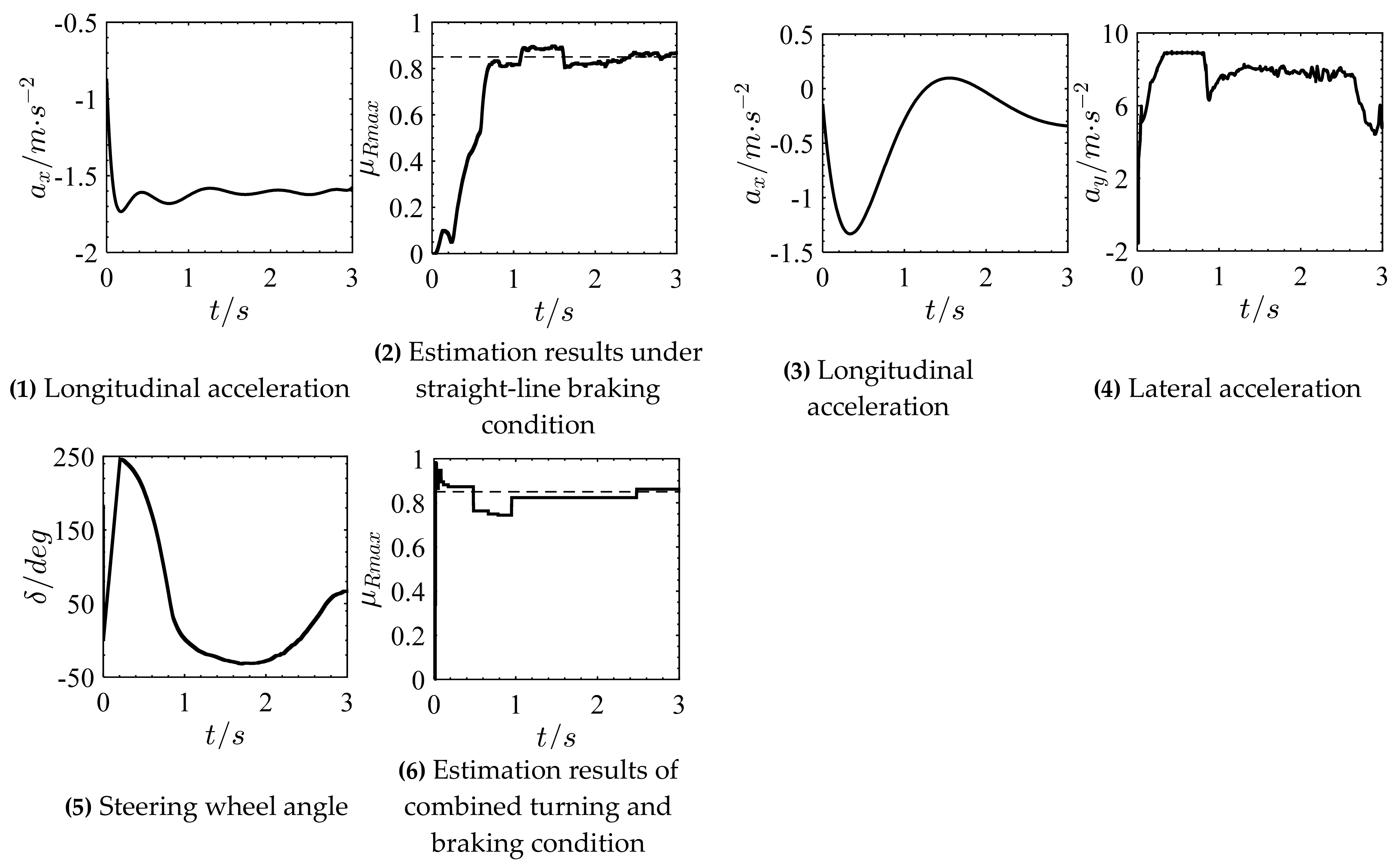
6.1. Straight-Line Braking Condition

The TRPFC was set to 0.85, the initial speed was 120 km/h, and the straight-line braking [49] condition was set. The B-level 3D road excitation data were used as the signal input. Taking the left front wheel as an example, the simulation results are given in Figure 7(1),(2).

From Figure 7(1),(2), it can be seen that the maximum longitudinal acceleration could reach −1.75 m/s² and that the TRPFC converged to 0.8 before 0.8 s and then fluctuated around 0.85, but the overall error was maintained in [−0.05, 0.05].

6.2. Combined Turning and Braking Condition

The experimental road was circular, the radius was 30 m, the TRPFC was set to 0.85, the initial speed was 60 km/h, and the combined turning and braking condition [50] is set. Taking the left front wheel as an example, the simulation results are shown in Figure 7(3)–(6).

From Figure 7(3)–(6), it can be seen that the maximum longitudinal acceleration could reach −1.35 m/s², the maximum lateral acceleration could reach 9 m/s², and the TRPFC converged to 0.9 after 0.2 s. After that, it fluctuated around 0.85 and was generally stable.

7. Real Vehicle Test

7.1. Real Vehicle Test Platform

As shown in Figure 8, the test platform was a wire-controlled modified utility vehicle (UTV, from RONGJUNTECH) with a four-wheel independent drive. The vehicle was equipped with a variety of sensors to obtain the test results. The sensors included GPS, inertial guidance (XSENS MTi-G-710), wheel speed sensors, and a steering wheel angle sensor.

7.2. Straight-Line Test

As shown in Figure 8, the straight-line driving condition [49] on a dry asphalt road was set. The peak friction coefficient between the tire and the dry asphalt road was in the range of [0.8,0.91] according to the available data [44], and the average test speed was 35 km/h. Taking the left front wheel as example, the test results are shown in Figure 9(1),(2).

From Figure 9(1),(2), it can be seen that the maximum longitudinal acceleration could reach 1.7 m/s² and that the TRPFC converged to 0.8 at about 0.3 s, then fluctuated steadily at about 0.86.

7.3. Curved Test

The experimental road was a dry asphalt circular road, the radius was 33.33 m, and the curved test [50] was set. The average test speed was 40 km/h. Taking the left front wheel as an example, the test results are shown in Figure 9(3)–(6).

From Figure 9(3)–(6), it can be seen that the longitudinal acceleration was up to 0.4 m/s², the lateral acceleration fluctuated between −2.2 m/s² and −1.4 m/s², and the steering wheel angle was up to 72 degrees. The TRPFC converged to 0.82 before 0.2 s and rose to about 0.87 after 0.6 s, then basically remained stable.

8. Conclusions

In the longitudinal and lateral directions, by combining the effective contact area ratio between the tire and the road with the LuGre tire model, a tire model considering the road surface texture was obtained. In the vertical direction, the single-point model was replaced by the multi-point contact model. The two models make up the 4.1. Vertical Dynamics Model. By combining the models with the UKF algorithm, the estimation result of the TRPFC was obtained.

From the simulation and experimental results, it can be seen that the proposed estimation algorithm can achieve an estimation of the TRPFC within 0.8 s, and the error can be maintained in [−0.05,0.05], whether in severe or steady daily conditions, which indicates that the proposed algorithm can estimate the TRPFC timely and accurately while considering the road texture.

Currently, the road is divided into eight grades from A to H. The estimation algorithm can adjust the estimation results according to the road grade to improve the estimation accuracy. All these contributions are important for promoting the development of vehicle active safety technology, improving the efficiency of road maintenance, alleviating the severe traffic situation, and reducing traffic accidents.

In the next step, the longitudinal–lateral–vertical coupling model of tire–road contact will be studied to further improve the estimation accuracy of the algorithm.

References

1. National Data Traffic Accident Statistics. China National Bureau of Statistics. 2021. Available online: https://data.stats.gov.cn/easyquery.htm?cn=C01&zb=A0S0D01&sj=2021 (accessed on 25 February 2022).
2. World Health Organization. Global Status Report on Road Safety 2015; World Health Organization: Geneva, Switzerland, 2015. [Google Scholar]
3. Chen, B.; Zhang, X.; Yu, J.; Wang, Y. Impact of contact stress distribution on skid resistance of asphalt roads. Constr. Build. Mater. 2017, 133, 330–339. [Google Scholar] [CrossRef]
4. Zhu, S.; Liu, X.; Cao, Q.; Huang, X. Numerical Study of Tire Hydroplaning Based on Power Spectrum of Asphalt Road and Kinetic Friction Coefficient. Adv. Mater. Sci. Eng. 2017, 2017, 1–11. [Google Scholar]
5. Wang, Y.; Hu, J.; Wang, F.; Dong, H.; Yan, Y.; Ren, Y.; Zhou, C.; Yin, G. Tire Road Friction Coefficient Estimation: Review and Research Perspectives. Chin. J. Mech. Eng. 2022, 35, 1–11. [Google Scholar] [CrossRef]
6. Guo, F.; Pei, J.; Zhang, J.; Li, R.; Zhou, B.; Chen, Z. Study on the skid resistance of asphalt pavement: A state-of-the-art review and future prospective. Constr. Build. Mater. 2021, 303, 124411. [Google Scholar] [CrossRef]
7. Mendoza-Petit, M.F.; Garcia-Pozuelo, D.; Diaz, V.; Garrosa, M. Characterization of the loss of grip condition in the Strain-Based Intelligent Tire at severe maneuvers. Mech. Syst. Signal Processing 2021, 168, 108586. [Google Scholar] [CrossRef]
8. Matsuzaki, R.; Kamai, K.; Seki, R. Intelligent tires for identifying coefficient of friction of tire/road contact surfaces using three-axis accelerometer. Smart Mater. Struct. 2015, 24, 025010. [Google Scholar] [CrossRef]
9. Kim, M.-H.; Park, J.; Choi, S. Road Type Identification Ahead of the Tire Using D-CNN and Reflected Ultrasonic Signals. Int. J. Automot. Technol. 2021, 22, 47–54. [Google Scholar] [CrossRef]
10. Yoon, J.-H.; Li, S.E.; Ahn, C. Estimation of vehicle sideslip angle and tire-road friction coefficient based on magnetometer with GPS. Int. J. Automot. Technol. 2016, 17, 427–435. [Google Scholar] [CrossRef]
11. Khaleghian, S.; Emami, A.; Taheri, S. A technical survey on tire-road friction estimation. Friction 2017, 5, 123–146. [Google Scholar] [CrossRef] [Green Version]
12. Zhang, Z.; Zheng, L.; Wu, H.; Zhang, Z.; Li, Y.; Liang, Y. An estimation scheme of road friction coefficient based on novel tyre model and improved SCKF. Veh. Syst. Dyn. 2021, 60, 2775–2804. [Google Scholar] [CrossRef]
13. Gustafsson, F. Slip-based tire-road friction estimation. Automatica 1997, 33, 1087–1099. [Google Scholar] [CrossRef]
14. Gustafsson, F. Monitoring tire-road friction using the wheel slip. IEEE Control Syst. 1998, 18, 42–49. [Google Scholar]
15. Wang, J.; Alexander, L.; Rajamani, R. Friction Estimation on Highway Vehicles Using Longitudinal Measurements. J. Dyn. Syst. Meas. Control 2004, 126, 265–275. [Google Scholar] [CrossRef]
16. Germann, S.; Wurtenberger, M.; Daiss, A. Monitoring of the friction coefficient between tire and road surface. In Proceedings of the IEEE Conference on Control Applications, Scotland, UK, 24–26 August 1994; IEEE: Piscataway, NJ, USA, 1994; pp. 613–618. [Google Scholar]
17. de Castro, R.; Araujo, R.E.; Cardoso, J.S.; Freitas, D. A new linear parametrization for peak friction coefficient estimation in real time. In Proceedings of the Vehicle Power and Propulsion Conference, Lille, France, 1–3 September 2010; IEEE: Piscataway, NJ, USA, 2010; pp. 1–6. [Google Scholar]
18. Wang, B.; Guan, H.; Lu, P.; Zhang, A. Road surface condition identification approach based on road characteristic value. J. Terramechanics 2014, 56, 103–117. [Google Scholar] [CrossRef]
19. Xin, W.; Liang, G.; Mingming, D.; Xiaolei, L. State estimation of tire-road friction and suspension system coupling dynamic in braking process and change detection of road adhesive ability. Proc. Inst. Mech. Eng. Part D J. Automob. Eng. 2021, 236, 1170–1187. [Google Scholar] [CrossRef]
20. Li, G.; Fan, D.S.; Wang, Y.; Xie, R.C. Study on vehicle driving state and parameters estimation based on triple cubature Kalman filter. Int. J. Heavy Veh. Syst. 2020, 27, 126–144. [Google Scholar] [CrossRef]
21. Sharifzadeh, M.; Senatore, A.; Farnam, A.; Akbari, A.; Timpone, F. A real-time approach to robust identification of tire–road friction characteristics on mixed-μ roads. Veh. Syst. Dyn. 2018, 57, 1338–1362. [Google Scholar] [CrossRef]
22. Gao, L.; Xiong, L.; Lin, X.; Xia, X.; Liu, W.; Lu, Y.; Yu, Z. Multi-sensor Fusion Road Friction Coefficient Estimation During Steering with Lyapunov Method. Sensors 2019, 19, 3816. [Google Scholar] [CrossRef] [Green Version]
23. Chu, L.; Cui, X.; Zhang, K.; Fwa, T.F.; Han, S. Directional Skid Resistance Characteristics of Road Pavement: Implications for Friction Measurements by British Pendulum Tester and Dynamic Friction Tester. Transp. Res. Rec. J. Transp. Res. Board 2019, 2673, 793–803. [Google Scholar] [CrossRef]
24. Uz, V.E.; Gökalp, I. Comparative laboratory evaluation of macro texture depth of surface coatings with standard volumetric test methods. Constr. Build. Mater. 2017, 139, 267–276. [Google Scholar] [CrossRef]
25. Bitelli, G.; Simone, A.; Girardi, F.; Lantieri, C. Laser Scanning on Road Pavements: A New Approach for Characterizing Surface Texture. Sensors 2012, 12, 9110–9128. [Google Scholar] [CrossRef] [PubMed]
26. Vollor, T.W.; Hanson, D.I. Development of Laboratory Procedure for Measuring Friction of HMA Mixtures—Phase I. Final Report of NCAT 06–06 (2006); National Center for Asphalt Technology, Auburn, Alabama, 2006.
27. Xu, H.; Prozzi, J.A. Correlation of aggregate form properties with fourier frequencies. Transp. Res. Rec. J. Transp. Res. Board 2020, 2674, 405–419. [Google Scholar] [CrossRef]
28. Wang, D.; Liu, P.; Xu, H.; Kollmann, J.; Oeser, M. Evaluation of the polishing resistance characteristics of fine and coarse aggregate for asphalt road using wehner/schulze test. Constr. Build. Mater. 2018, 163, 742–750. [Google Scholar] [CrossRef]
29. Hu, L.; Yun, D.; Gao, J.; Tang, C. Monitoring and optimizing the surface roughness of high friction exposed aggregate cement concrete in exposure process. Constr. Build. Mater. 2020, 230, 117005. [Google Scholar] [CrossRef]
30. Hao, X.; Sha, A.; Sun, Z.; Li, W.; Zhao, H. Evaluation and comparison of real-time laser and electric sand-patch road texture-depth measurement methods. J. Transp. Eng. 2016, 142, 04016022. [Google Scholar] [CrossRef]
31. Gökalp, I.; Uz, V.E.; Saltan, M. Comparative laboratory evaluation of macro texture depth of chip seal samples using sand patch and outflow meter test methods. In Bearing Capacity of Roads, Railways and Airfields; CRC Press: Boca Raton, FL, USA, 2017; pp. 915–920. [Google Scholar] [CrossRef]
32. Zhu, H.; Liao, Y. Present situations of research on anti-skid property of asphalt road. Highway 2018, 63, 35–46. [Google Scholar]
33. Grosch, K.A. Visco-Elastic Properties and the Friction of Solids: Relation between the Friction and Visco-elastic Properties of Rubber. Nature 1963, 197, 858–859. [Google Scholar] [CrossRef]
34. Adam, C.S.; Piotrowski, M. Use of the unified theory of rubber friction for slip-resistance analysis in the testing of footwear outsoles and outsole compounds. Footwear Sci. 2012, 4, 23–35. [Google Scholar] [CrossRef]
35. Mazzola, L.; Galderisi, A.; Fortunato, G.; Ciaravola, V.; Giustiniano, M. Influence of Surface Free Energy and Wettability on Friction Coefficient between Tire and Road Surface in Wet Conditions. Adv. Contact Angle Wettability Adhes. 2013, 1, 389–410. [Google Scholar] [CrossRef]
36. Persson, B.N. Rubber friction: Role of the flash temperature. J. Phys. Condens. Matter 2006, 18, 7789–7823. [Google Scholar] [CrossRef]
37. Ueckermann, D.; Wang, M.; Oeser, B. Steinauer, Calculation of skid resistance from texture measurements. J. Traffic Trans. Eng. 2015, 2, 3–16. [Google Scholar]
38. Hertz, H. On the contact of elastic solids. J. Die Reine Angew. Math. 1882, 92, 156–171. [Google Scholar] [CrossRef]
39. Greenwood, J.A.; Williamson, J. Contact of nominally flat surfaces. Proc. R. Soc. Lond. 1966, 295, 300–319. [Google Scholar]
40. Carbone, G. A slightly corrected Greenwood and Williamson model predicts asymptotic linearity between contact area and load. J. Mech. Phys. Solids 2009, 57, 1093–1102. [Google Scholar] [CrossRef]
41. Persson, B.N.J. Theory of rubber friction and contact mechanics. J. Chem. Phys. 2001, 115, 3840–3861. [Google Scholar] [CrossRef] [Green Version]
42. Lu, Y.; Zhang, J.; Yang, S.; Li, Z. Study on improvement of LuGre dynamical model and its application in vehicle handling dynamics. J. Mech. Sci. Technol. 2019, 33, 545–558. [Google Scholar] [CrossRef]
43. Yongjie, L.; Junning, Z.; Haoyu, L.; Zhizhe, M. Research on tire-road system coupling dynamics based on non-uniform contact. J. Mech. Eng. 2021, 57, 87–98. (In Chinese) [Google Scholar]
44. Yongjie, L.; Wenqing, H.; Junning, Z. Construction of Three-Dimensional Road Surface and Application on Interaction between Vehicle and Road. Shock Vib. 2018, 2018, 1–14. [Google Scholar] [CrossRef] [Green Version]
45. Han, Y.; Lu, Y.; Chen, N.; Wang, H. Research on the Identification of Tire Road Peak Friction Coefficient under Full Slip Rate Range Based on Normalized Tire Model. Actuators 2022, 11, 59. [Google Scholar] [CrossRef]
46. Kiencke, U.; Nielsen, L. Automotive Control Systems: For Engine, Driveline, and Vehicle; Springer: Berlin/Heidelberg, Germany, 2005. [Google Scholar]
47. Rajamani, R. Vehicle Dynamics and Control, 2nd ed.; Springer Science: London, UK, 2012. [Google Scholar]
48. Mechanical Vibration-Road Surface Profiles-Reporting of Measured Data; Standardization Administration: Beijing, China, 2006.
49. Standard’s ISO 21994-2007; Standard’s Passenger Cars-Stopping Distance at Straight-Line Braking with ABS-Openloop Test Method. ISO: Geneva, Switzerland, 2007.
50. Standard’s ISO 4138:2004; Standard’s Circular Driving Behaviour—Open-Loop Test Methods. ISO. ISO: Geneva, Switzerland, 2012.
Figure 1. Estimation flowchart for TRPFC.
Machines 10 00614 g001
Figure 2. Vehicle dynamics model.
Machines 10 00614 g002
Figure 3. Tire–road vertical dynamics model.
Machines 10 00614 g003
Figure 4. Quarter suspension model.
Machines 10 00614 g004
Figure 5. A-H-level 3D road reconstruction results.
Machines 10 00614 g005
Figure 6. UKF estimation flowchart.
Machines 10 00614 g006
Figure 7. Simulation results.
Machines 10 00614 g007
Figure 8. Real vehicle test platform.
Machines 10 00614 g008
Figure 9. Real vehicle test results.
Machines 10 00614 g009