Article

Sequential Reliability Analysis for the Adjusting Mechanism of Tail Nozzle Considering Wear Degradation

1
School of Mechanics, Civil Engineering and Architecture, Northwestern Polytechnical University, Xi’an 710072, China
2
Xi’an Aerospace Propulsion Institute, Xi’an 710100, China
*
Author to whom correspondence should be addressed.
Machines 2022, 10(8), 613; https://doi.org/10.3390/machines10080613
Submission received: 18 June 2022 / Revised: 15 July 2022 / Accepted: 22 July 2022 / Published: 26 July 2022
(This article belongs to the Special Issue Reliability Evaluation for Industrial Systems: State of the Art)

Abstract

:
The adjusting mechanism is an important part of an aero engine, and the wear degradation of clearance is widely present in its hinges. In this work, an adjusting mechanism with hinge clearance is analyzed by dynamic simulation and the wear depth is predicted precisely using a wear model. Based on that, a sequential reliability analysis of motion accuracy is carried out. In order to avoid the expensive computational cost of simulation, the adaptive radial-based importance sampling method combined with the adaptive Kriging model (AK-ARBIS) is employed, which describes the decrease of reliability in the standard normal space sphere by sphere with the updated Kriging model. To further utilize the information about each state of wear degradation, the advanced AK-ARBIS method is investigated. Through analytical examples of two typical mechanisms and the engineering application of the adjustment mechanism, the results show that the calculation cost of the sequential reliability analysis under different states can be effectively reduced.

1. Introduction

When aero engines meet the requirements of different tasks, the adjusting mechanism of the tail nozzle must be used to complete the redistribution of engine flow, so as to achieve the change of engine performance [1,2]. The adjusting mechanism is a typical multistate linkage with complex working conditions, which requires high precision of initial machining and assembly [3]. Due to the influence of friction and wear in the process of operation, it is easy to produce clearance between each pair of connecting rods [4,5]. This will significantly affect the motion accuracy of the adjusting mechanism and lead to failure events [6]. Therefore, the motion accuracy and reliability of the adjusting mechanism with clearance is an important factor that affects the normal operation of the engine, which poses a serious threat to flight safety.
The clearance wear may commonly and sharply deteriorate the motion accuracy caused by a slight deviation, especially in high-precision mechanisms. At present, many works are focused on the clearance wear of mechanisms, which is expected to be precisely evaluated [7,8]. For instance, Lai et al. [7] proposed an effective iterative prediction method to calculate the wear of rotating hinges for planar mechanisms, which is verified by wear data from typical mechanisms. Bai et al. [9] used the hybrid nonlinear contact force model and the modified Coulomb friction model for clearance wear. Geng et al. [10] combined wear prediction and multi-body dynamics analysis of non-uniform rotational hinge clearance. Li et al. [11] proposed a solution strategy based on the Monte Carlo method to study the kinematic and dynamic characteristics of spatial deployable mechanisms with hinge clearance, which demonstrated that the effect of parameter uncertainty makes the evaluation more accurate. A more comprehensive survey of analytical, numerical and experimental methods for mechanism systems with hinge clearance is presented in a review by Tian et al. [12]. In the above literature, it is pointed out that wear degradation is an important factor concerning the motion accuracy of mechanisms. Based on previous work, by dividing the non-uniform wear contact area of the pins into discrete intervals of a single cycle and analyzing the motion in the framework of multi-body dynamics simulation, the wear depth for the clearance of the adjusting mechanism can be predicted precisely according to the Archard model [10].
Considering wear clearance, reliability analysis of mechanisms has attracted more attention from researchers, especially for the highly reliable mechanical products with degradation [13,14]. Wu et al. [15] proposed an indirect probability model (IPM) that comprehensively evaluates the reliability of multi-body mechanisms. Li et al. [16] considered the degradation performance caused by wear and multi-source uncertainties, and the reliability analysis was developed for aircraft lock mechanisms. The research of reliability analysis theory is relatively mature and has been applied in various professional fields. However, these researchers did not study the reliability analysis methods of clearance hinges in different states of wear degradation. In practical engineering, the performance function is mostly highly nonlinear and the numerical response is usually obtained by dynamic simulation. Especially for the degenerate time-varying reliability [8,17], it is a time-nested loop process where each time increment corresponds to constructing a performance function, which is time-consuming and difficult to handle. Therefore, based on the reliability method, this paper mainly conducts sequential reliability analysis for the different states of wear degradation.
To construct the real performance function in each wear state for reliability analysis, the surrogate model is often used, which greatly improves the computational efficiency. Recently, a popular method is the AK-MCS method, which uses the adaptive Kriging (AK) model combined with Monte Carlo simulation (MCS) to calculate reliability [18,19,20]. To further accelerate the Kriging model’s convergence, Zheng et al. [21] proposed a new active U learning function in AK-MCS, and Hu et al. [22] proposed taking the maximum error percentage of failure probability estimation as the convergence criterion. In order to solve the problem of a large candidate sample pool of AK-MCS, some importance sampling methods combining AK models to reduce variance are proposed, such as AK-IS (importance sampling) [23,24], AK-SS (subset simulation) [25,26], AK-ARBIS (adaptive radial-based importance sampling) [27,28,29] and other advanced methods [30,31,32]. Based on the AK-ARBIS method proposed by scholars, this paper further improves and applies the method to the sequential reliability analysis of mechanism with wear degradation. Since the wear process is characterized by sequential degradation, reliability commonly decreases with the degradation procedure. Gradually inward from the margin in the standard normal space, the Kriging models for different degradation states can be updated between spheres. Additionally, the Kriging model information from previous states can be used to further reduce the number of calls to the dynamic simulation. The proposed sequential reliability analysis combines the hierarchical idea of ARBIS and the strong predictability of AK. With this improved method, the candidate samples in the standard normal space are reduced, and the computational efficiency and the prediction accuracy under different degradation states are improved.
The remaining structure of this paper is as follows. Section 2 introduces dynamic simulation of the adjusting mechanism and predicts the wear depth of clearance. Section 3 introduces the details of sequence reliability analysis AK-ARBIS under wear degradation. Two analytical examples of a four-link mechanism and a steering mechanism are analyzed in Section 4. In Section 5, the sequential reliability analysis of the adjusting mechanism under different clearance degenerate states is carried out. Finally, the conclusion is summarized in Section 6.

2. Dynamic Analysis for the Adjusting Mechanism

2.1. Introduction of Adjusting Mechanism Model

The adjusting mechanism is an important mechanical part in the tail nozzle of an aircraft engine. It controls the angle of the scale blade through mechanical adjustment, which can change the steering direction of the tail nozzle to adjust the thrust direction and size. The adjusting mechanism directly affects the performance, maneuverability and reliability of aircraft.
As seen in Figure 1, the adjusting mechanism of the tail nozzle is composed of 12 groups of sub-mechanisms arranged with equal ring spacing, and the geometric boundary conditions are symmetric. In order to simplify the analysis, only one twelfth of the adjusting mechanism, namely a fan-shaped symmetric model, is selected as the research object. The simplified adjusting mechanism is the solid model shown in Figure 1, which includes the adjusting ring, connecting rod, scale blade and other structures. Due to the high stiffness of the component materials, deformation can be ignored and the components are regarded as rigid bodies. The working principle of this mechanism is summarized as follows: the hydraulic actuator provides the driving force to control the adjustment ring, and the movement of adjustment ring drives the rotation of the connecting rod, and then controls the adjustment of the angle of the scale blade through the hinge. The movement of this mechanism is carried out by multi-body dynamics simulation analysis.

2.2. Clearance Degradation of Adjusting Mechanism

Although the structure of this adjusting mechanism is relatively simple, due to the high movement frequency and harsh working conditions, the pin at the hinge is rapidly worn by friction and collision, resulting in the gap between the pin and the bushing increasing. With this degradation, the motion accuracy of this mechanism maybe inadequate, which leads to the loss of performance of the engine. Therefore, it is necessary to investigate the influence of the degradation of clearance for the adjusting mechanism.

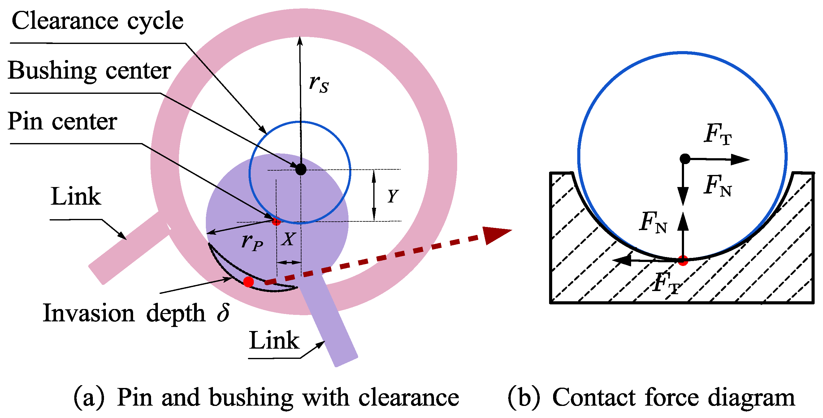
2.2.1. Theoretical Model of Contact Force in Clearance

As shown in Figure 2, with the movement of the mechanism, the center of the pin and the bushing do not overlap completely, and clearance exists between them. If the pin and bushing are all of ideal rigid body, the relative position of their center is changed with the rotation but the clearance is the same, which can be described by the clearance cycle. However, in real cases, due to the contact force between the pin and bushing, there is an extremely small invasion, which will lead to degradation with the number of rotations increasing. For hinges, the stiffness of the pin is often higher than that of the bushing in engineering practice, so the pin is assumed to be a rigid body. The bushing has a larger contact area and lower stiffness than the pin, and its wear depth is very small, so its deformation is not considered here. In order to make clear the law of degradation based on this assumption, the contact force is first discussed.
The contact forces in the hinge clearance include the normal pressure F N and tangential friction force F T , then the total contact force can be given by
F = n N F N + n T F T
where n N , n T are the unit normal vector and unit tangent vector, respectively.
The normal pressure is related to the relative velocity, material properties, geometric properties, deformation and other factors. The equivalent spring damping method [7] is used to deal with the nonlinear continuous dynamics of contact, and the normal pressure is expressed as
F N = κ δ e + D δ ˙
where κ is the generalized stiffness coefficient depending on material properties and contact surface shape, δ is the depth of invasion, e is the nonlinear rigidity index, which is related to the material type of contact bodies, δ ˙ is the relative velocity, and D is the damping coefficient.
For the tangential friction force F T , the coulomb friction model [7] is adopted which is given by
F T = μ F N ν T ν T
where μ is the friction coefficient and ν T is the relative tangential velocity.
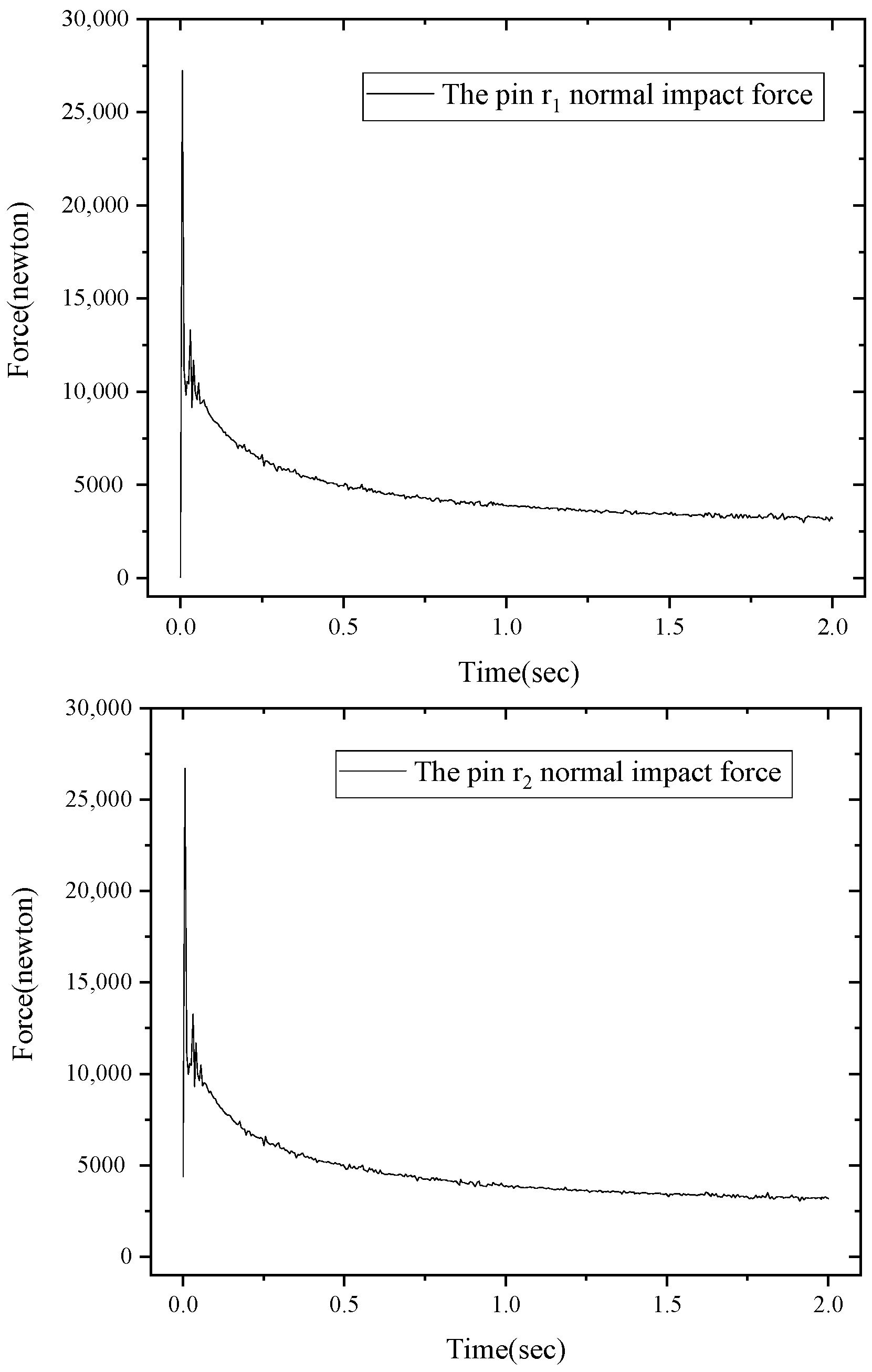
In real practice, the contact force in the clearance is always analyzed by multi-body dynamics simulation. For the adjusting mechanism, the total motion for the adjustment angle of the scale blade is shown in Figure 3. It is seen that the scale blade rotates from the initial angle 13° to the terminal angle 45° within 2 s. In this procedure, the normal pressures at two pin shafts are obtained, which are shown in Figure 4. It is seen that in the startup phase, the forces sharply increase, but with the rotation, the forces decrease gradually.

2.2.2. Wear Degradation of Pins

At present, most studies regard wear degradation as uniform wear to simplify the analysis, but in actual engineering practice, the wear degradation process is always complex and shows the non-uniform wear phenomenon. Therefore, this work adopts the widely used Archard model to predict the wear depth. This model establishes the relationship between the wear depth and the load, sliding distance and hardness, and it is generally given by
V S = K H F N
where V is the wear volume, S is the relative sliding distance, K is the wear coefficient, H is the hardness of the material, usually taken as H 3 σ s , σ s is the yield strength of the material. Dividing both sides of the above formula by the contact area, the wear depth can be obtained by
h = K H A c F N S
where h is the wear depth, A C is the equivalent contact area.
When the mechanism is in a stable wear state, the pin and bushing are in continuous contact with relative invasion. Therefore, based on the clearance contact model in this paper, the contact length is calculated as follows.
As shown in Figure 5a, the wear invasion of pin and bushing is δ . The equivalent contact area A C in an increment region can be represented by the product of its transverse projection A B and the contact width w , which is given by
A c = A B × w
According to Figure 5a, A B can be obtained by
A B = O j A 2 + O j B 2 2 O j A O j B cos ( 2 Δ α ) = 2 R j 2 [ 1 cos ( 2 Δ α ) ]
where Δ α is the increment angle.
In the whole motion procedure, the wear contact area can be divided into discrete intervals. As shown in Figure 5b, the pin rotates an increment angle Δ α in time interval Δ t . Thus, when the whole motion rotates as angle α , all the discrete intervals can be denoted as
0 , Δ α , Δ α , 2 Δ α , ( N t 1 ) Δ α , N t Δ α , N t = α Δ α
where N t is the number of increment angles. Therefore, in any interval ( i 1 ) Δ α , i Δ α , the wear depth is given by
Δ h = K H A c F N Δ S
where Δ S is the sliding distance, and Δ h is the wear depth in an increment angle.
To measure the wear depth of each rotation, the average wear depth in a single cycle is given by
h = α 2 π ( 1 N t i = 1 N t Δ h )
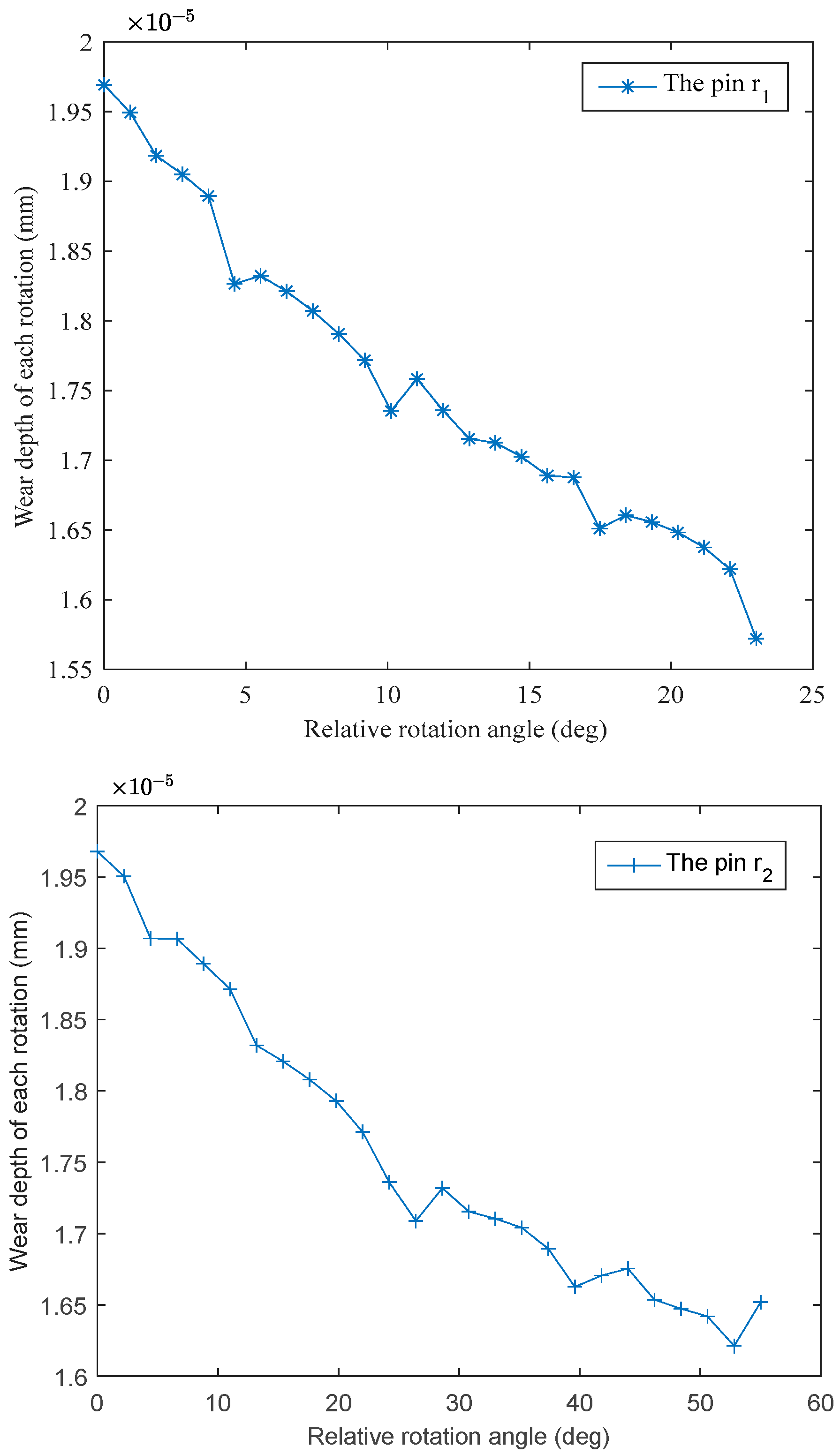
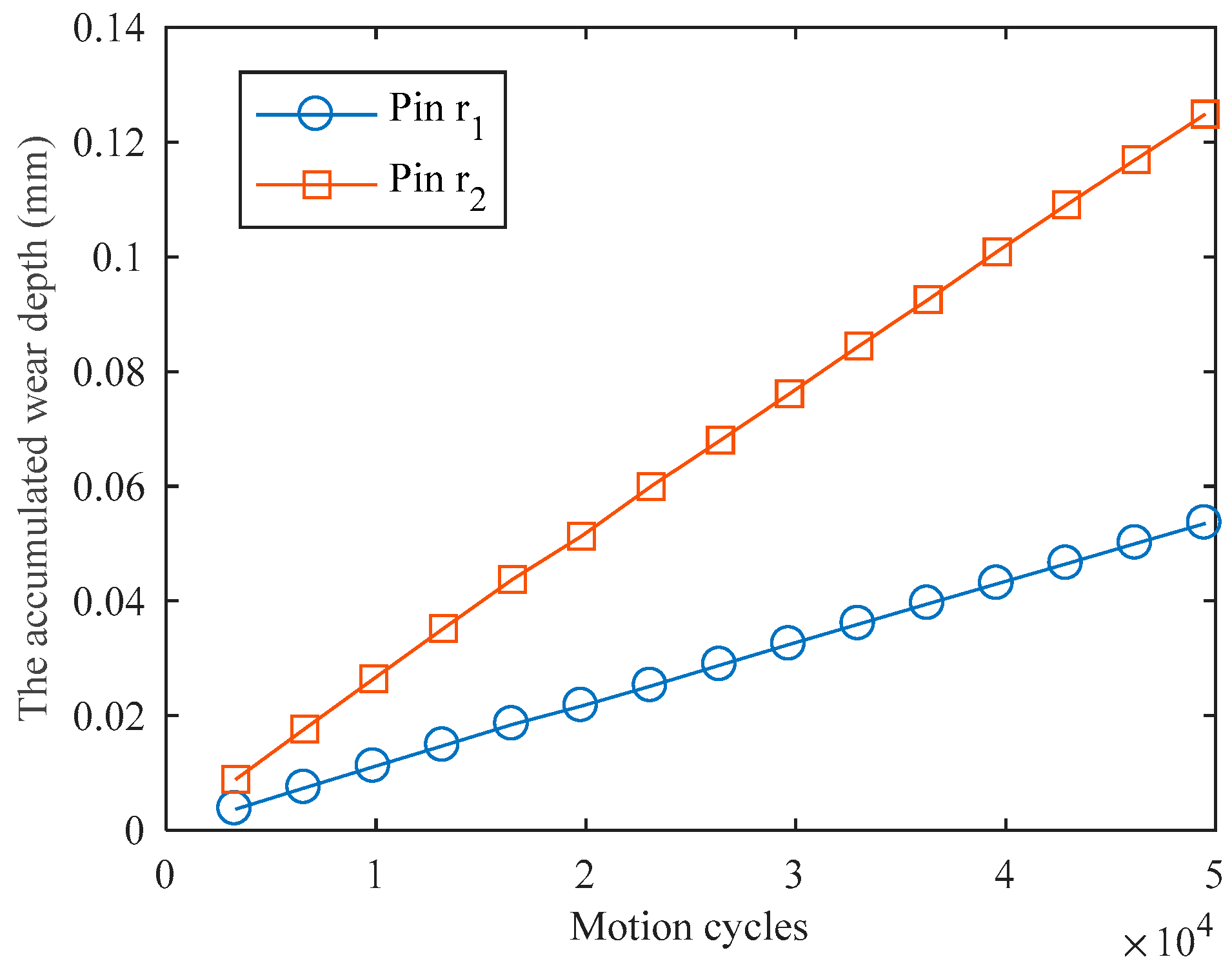
As shown in Figure 6, in the contact area of the relative rotation angle, the wear depth of each discrete interval of the two pins is given. Obviously, the wear of the pin is non-uniform, and the trend of the curve is mainly consistent with the curve of normal pressure of the pin in Figure 4. To predict the wear depth in a certain service life, the total running time is composed of a series of motion cycles. At each motion cycle, the wear depth can be computed by Equation (10), where the related parameters such as the normal pressure can be obtained by multi-body dynamics simulation. Then, the accumulated wear depth can be computed easily in a certain service life.
Since the adjusting mechanism in this work belongs to a high-precision mechanism and the surface of the component has been grinded with high precision before assembly, then the whole wear degradation process of the pin is in a stable wear state. As is seen from Figure 7, the wear depth of the clearance of the pin has an approximate linear relationship with the running time. In practical application, when the mechanism has exceeded the state of severe wear, its reliability is also significantly reduced beyond a certain threshold. For the sake of safety, the pins and other parts must be repaired or replaced or directly scrapped.

3. Sequential Reliability Analysis Considering Clearance Degradation

3.1. Reliability Analysis with Surrogate Model

The clearance of the mechanism is inherent arising from manufacturing and assembling. The slight deviation of clearance can lead to a dramatic loss of motion accuracy for the high-precision adjusting mechanism. Due to the existence of uncertainties, it is necessary to investigate the reliability of the adjusting mechanism with clearance. Generally, the performance function of a mechanism can be denoted as Y = g ( X ) , where X = ( X 1 , X 2 , , X m ) are m-dimensional random variables such as clearance variables. Then, the failure probability can be generally denoted as
P f = I F ( X ) f X X 1 , , X m d X 1 d X m
where f X X 1 , , X m is the joint probability density function (PDF), and I F ( X ) = 1 x F   0 x F is the indicator function of failure domain F .
For the reliability analysis of the adjusting mechanism, the surrogate model-based method can be employed to estimate the failure probability efficiently. Recently, the Kriging model is preferable with the capacity to achieve the prediction mean and variance, which can be denoted as g N ( μ g K ( X ) ,   σ g K 2 ( X ) ) , where μ g K ( X ) is the predication mean and σ g K 2 ( X ) is the corresponding variance. Based on that, a great deal of learning functions have been proposed to actively update the Kriging model, such as information entropy based function [18], probabilistic classification function [19], U learning function [20], expected feasibility function (EFF) [33], maximum confidence enhancement function [34], etc. A comprehensive comparison of those learning functions is given in references [18,35,36]. In this work, the popular U learning function is employed to update the Kriging model, which can be given as
U ( X ) = μ g K ( X ) σ g K ( X )
The learning function can be used to find the best candidate sample points to improve the accuracy of the original Kriging model, namely:
x b e s t = arg   min k = 1 , , N   U ( x k )
where N is the number of candidate samples.
The convergence stop criterion [29] can be taken as min k = 1 , , N U ( x k ) 2 . The accuracy of the original Kriging method can be greatly improved by using the learning function.
The Kriging model is intuitive and easy to combine with the MCS method, but the disadvantage is that the sample information is not effectively utilized to capture the failure region. To improve the computational efficiency, advanced sampling methods, such as IS, LS, ARBIS, etc. are combined with the Kriging model, which show advantages to estimate the small failure probability. Those methods are widely employed to compute the reliability of the adjusting mechanism with the uncertainty of clearance.

3.2. Reliability Model Considering Clearance Degradation

When considering the clearance degradation of the adjusting mechanism, the radius of the pin keeps decreasing, which causes variation in the clearance parameters. Generally, for the high-precision adjusting mechanism, the failure probability at the beginning state is small, but with clearance degradation, the failure probability of the adjusting mechanism will increase sequentially. As shown in Figure 8a, the sample space is changed with the variation of clearance parameters, which induces the increase of failure probability. Nevertheless, the physical relationship between clearance parameters and output commonly remains the same. This indicates that the Kriging model for the performance function needs to be updated in different sample spaces, which needs to use a great deal of candidate samples. In a large-scale candidate sample pool, the adaptive selection of sample points will be time-consuming.
However, when the original sample space is transformed into the standard normal space by equivalent probability transformation, namely F ( x | θ ) = Φ ( u ) , where F ( ) and Φ ( ) are the cumulative distribution functions (CDF) of original distribution and standard normal distribution, and θ represents the distribution parameters corresponding to the different degradation states, then the performance functions in the standard normal space can be denoted g ( F 1 ( Φ ( u ) | θ ) as H u , θ , which are changed with the degradation parameters θ . In order to simplify the description, the performance functions are denoted as H i ( u )   ( i = 1 , 2 , ) in the following. As shown in Figure 8b, the original performance function g ( X ) in different degradation sample spaces can be converted into a series of H i ( u ) in the standard normal space, which reflects the variation of failure probability. Intuitively, H i ( u ) can directly describe the sequential degradation of the mechanism reliability, but this causes the problem that, when employing the Kriging-based method, it is necessary to construct a series of Kriging models. Nevertheless, since the Kriging models with the degradation of mechanism are sequentially changed, they have similar information from different degradation states which can be used to construct the models. Furthermore, the failure probability commonly increases with the degradation procedure, so it is appropriate to explore the standard normal space from the margin to the inner gradually. Therefore, the adaptive radial-based importance sampling combined with the Kriging model is investigated to calculate the sequential reliability of the mechanism in the following section.

3.3. Sequential Reliability Analysis Based on AK-ARBIS

3.3.1. AK-ARBIS Method

The core idea of ARBIS is to gradually search for the optimal sphere β o p t in the standard normal space layer by layer. The schematic diagram of this adaptive search is shown in Figure 9. For more details of the specific implementation process of the ARBIS method, readers can refer to [29]. Because the samples (red dots) inside the optimal sphere are absolutely safe there is no need to calculate their response values, which reduces the calculation cost greatly. To further improve the computational efficiency, the active learning Kriging model is embedded in the iteration of spheres and the AK-ARBIS method is established for the estimation of small failure probability. The Kriging model is constructed with the points out of the initial sphere and updated with the contributive points of each layer. The concrete steps for the update of the Kriging model can be seen in [20].

3.3.2. Advanced AK-ARBIS for Sequential Reliability

Based on the AK-ARBIS method, it is worth noting that the problem of clearance degradation is accompanied by the decrease of reliability index, which is similar to the update of the Kriging model from the initial sphere to the optimal sphere. Therefore, the AK-ARBIS method is proposed in this section to solve the failure probability at each degenerate state. The difference is that for the sequential reliability analysis with clearance degradation, different Kriging models need to be constructed to predict the responses of each degenerate state. The more degenerate states are selected, the more Kriging models need to be constructed, which obviously increases the computational cost. Therefore, the original AK-ARBIS method is explored further in this section to make full use of the information between multiple Kriging models.
As shown in Figure 10, when the i-th state is implemented, the optimal sphere in the previous (i − 1)-th state can be used to further reduce the candidate sample pool. It can be used as the initial sphere for the i-th state to construct i-th Kriging model. Moreover, since the points near the (i − 1)-th Kriging model contain contributive information for the i-th state, those points can be used as the initial points for the i-th Kriging model, which avoids the random selection of the initial point for the i-th Kriging model and accelerates the convergence.
The specific calculation steps are as follows.
Step 1. Set the initial radius β 0 1 of the sphere, which can be set as
β 0 1 = χ n 2 1 p 0
where χ n 2 represents the inverse Chi-square distribution function with n degree of freedom, and P 0 represents the initial failure probability. It always takes a small value, generally P 0 = 10 6 , to ensure that the initial sphere intersects with the failure region.
Step 2. Generate samples in standard normal space.
According to the PDF φ ( u ) of the standard normal distribution, the sample of variables u k ( k = 1 , 2 , , N ) is generated.
Step 3. Construct the Kriging model in the initial degenerate state i = 1 .
Step 3a. For the samples outside the sphere u k β 0 1 , denoted as the set A 0 1 . The N K 0 1 samples are randomly selected from A 0 1 , and their corresponding response values are calculated by H 1 u k , θ .
Step 3b. Construct the Kriging model H K , 0 1 through the training sample set T = u 1 , H 1 u 1 , θ , , u N K 0 , H 1 u N K 0 , θ .
Step 3c. For the Kriging model, the next optimal sample u b e s t = arg min u k A 0 1 U ( u k ) and the corresponding response value H 1 u b e s t , θ are added to the training sample set T to update the Kriging model H K , 0 1 until the stop criterion min u k A 0 1 U ( u k ) 2 is met.
Step 3d. The updated Kriging model H K , 0 1 is used to estimate the response of samples A 0 1 . Then the results are saved and the number of failed samples, denoted as N f , 0 1 , are counted.
Step 3e. Determine the new sphere β l 1 .
For the failure samples selected outside the sphere u k β 0 1 , its PDF value φ ( u ) is calculated, and the point with the maximum PDF value is denoted as u 0 max . Then, the current updated Kriging model H K , l 1 1 can be used to calculate the new sphere β l 1 by solving the equation
H K , l 1 1 β l 1 u l 1 max u l 1 max = 0
Figure 9 shows the linear search process of the Kriging model for the new sphere. Since the Kriging model cannot be given analytically, the new sphere is found by adaptive linear search, and Equation (14) can be solved numerically, such as dichotomy.
Step 3f. Select the failure samples between the spheres.
For satisfied samples β l 1 u k β l 1 1 , update the Kriging model H K , l 1 to estimate its response, and then save the results and count the number of failure samples, denoted as N f , l 1 .
Step 3g. Repeat steps 3. e–f until the new sphere β l 1 is optimal when no failure samples are found between the corresponding spheres. In this process, all the failure samples in this degenerate state can be found. Then, the failure probability and its coefficient of variation C.O.V can be calculated in the following way.
P ^ 1 f = N f , l 1 N C o v P ^ 1 f = 1 P ^ 1 f N P ^ 1 f
If the C o v P ^ f 1 exceeds 0.05, the sample size should be expanded and the above steps repeated.
Step 4. Construct the Kriging model in the i-th degenerate state.
Step 4a. Let the optimal sphere radius β l i 1 in the previous state be equal to the initial radius β 0 i in current state. For the samples outside the sphere u k β 0 i , denoted as the set A 0 i . Note that the N K 0 i samples are not randomly selected, but samples close to the previous Kriging model are selected from A 0 i , where their corresponding response values were calculated by H i u k , θ .
Step 4b. Construct the Kriging model H K , 0 i through the training sample set T = u 1 , H i u 1 , θ , , u N K 0 , H i u N K 0 , θ .
Step 4c. Update the Kriging model H K , 0 i by adding the next optimal sample u b e s t = arg min u k A 0 i U ( u k ) and the corresponding response value H i u b e s t , θ until the stop criterion min u k A 0 i U ( u k ) 2 is met.
Step 4d. Estimate the response of samples A 0 i and count the number of failure samples N f , 0 i using the updated Kriging model H K , 0 i .
Step 4e. For the failure samples outside the sphere u k β 0 i , select the point with the maximum PDF value as u 0 max . Similar to step 3. e, determine adaptively the new sphere β l i using the currently updated Kriging model H K , l 1 i .
Step 4f. Select the failure samples between the spheres β l i u k β l 1 i to update the Kriging model H K , l i , then estimate its response and count the number of failure samples N f , l i .
Step 4g. Repeat steps 4. e–f until the new sphere β l i is optimal when no failure samples are found between the corresponding spheres. Then similar to Equation (15), the failure probability P ^ f i and its coefficient of variation C o v P ^ f i can be calculated.
It can be seen from the above process that the proposed method transforms the sample space of different states into a standard normal space and uses the Kriging model to iterate step by step to predict the number of failure samples between the sphere layers, thereby, the failure probability under different degenerate states is calculated. This method greatly reduces the size of the entire training sample pool and saves more time in the process of the updated Kriging model.

4. Validation Numerical Examples

In this section, two analytical mechanism examples are used to verify the accuracy and efficiency of the proposed method. The circle size of the hinge clearance involved is composed of two position variables and the mean values of them in different states increase step by step to represent the degradation of the variables. The results were calculated by the MCS, AK-MCS and AK-ARBIS methods, respectively, for comparison.

4.1. A Four-Bar Linkage Mechanism

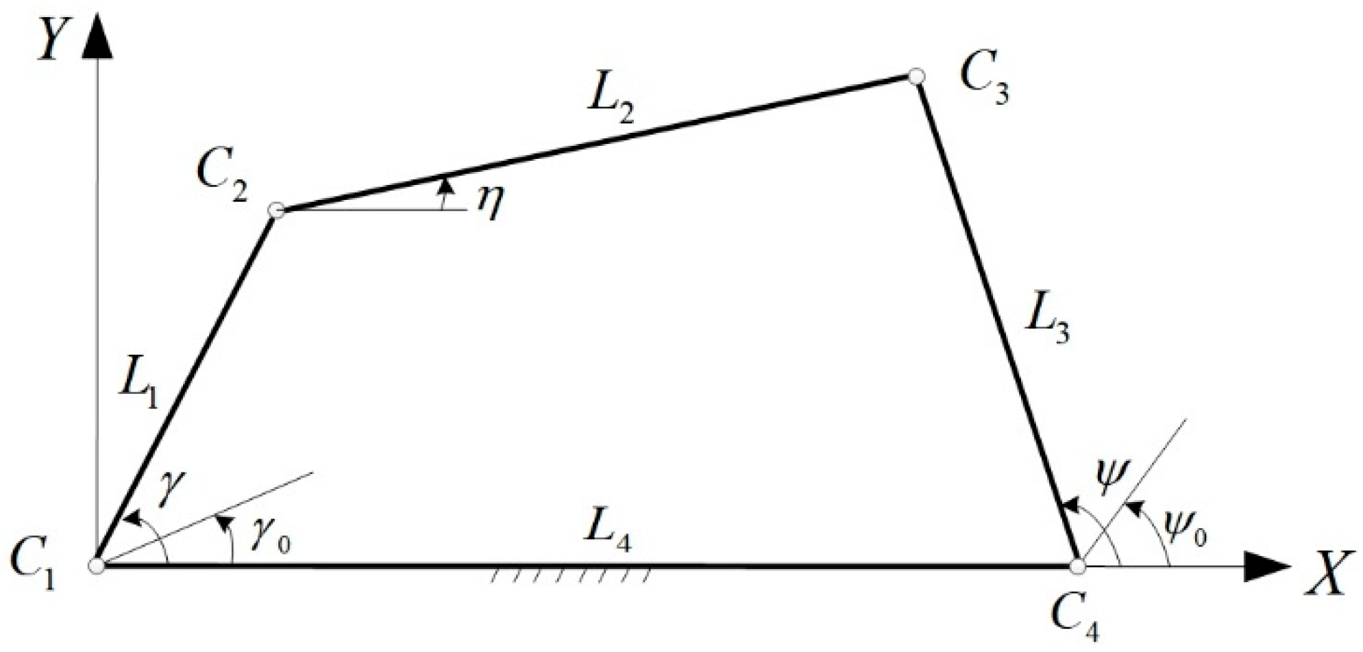
The schematic diagram of a four-bar linkage is shown in Figure 11. The frame rod L 4 is fixed, and the driving rod L 1 drives the rocker rod L 3 through the connecting rod L 2 . All the rods are connected by hinges and their lengths are 52.2, 104.9, 67.6 and 100 mm, respectively. It is assumed that the circular size C i X i , Y i of each hinge clearance is uniformly distributed within the circle and degenerates with the wear of the hinge. In this paper, Rosenblatt’s transformation method [37] is adopted to transform each pair of position variables into independent normal variables. The radius of the clearance circle can be given by r c i = X i 2 + Y i 2 . A reasonable assumption is made for the radius of the clearance circle in each state based on the reasonable amount of clearance wear. See Table 1 for specific values.
Thus, the kinematics equation of the four-bar linkage considering the clearance can be obtained
L 1 cos γ + L 2 cos η L 3 cos ψ L 4 + X 1 + X 2 X 3 X 4 = 0 L 1 sin γ + L 2 sin η L 3 sin ψ + Y 1 + Y 2 Y 3 Y 4 = 0
The actual motion output equation can be obtained by eliminating η
ψ = 2 arctan B + A 2 + B 2 C 2 C A
where
E = L 1 cos γ + L 4 + X 1 + X 2 X 3 X 4 F = L 1 sin γ + Y 1 + Y 2 Y 3 Y 4 A = 2 E L 3 B = 2 F L 3 C = E 2 + F 2 + L 3 2 L 2 2
In this paper, the mechanism failure for the motion accuracy is investigated. Therefore, the failure mode of the four-bar linkage is defined as: when the driving rod runs to γ = 215 × π 180   rad , the error between the actual positioning angle ψ t and the ideal positioning angle ψ i d of the rocker rod exceeds the threshold Δ = 0.02   rad . That is, the motion failure of the mechanism is identified; otherwise, it is safe.
Therefore, the performance function of four-bar linkage can be obtained as
g X i , Y i = Δ ψ i d ψ t ( i = 1 , 2 , 3 , 4 )
According to the above discussion, Table 2 gives the failure probability and the corresponding C.O.V value calculated by MCS, AK-MCS and the proposed AK-ARBIS method. When compared with the MCS method, the AK-ARBIS method and AK-MCS method have extremely high accuracy (the error is controlled within 5%), but the AK-ARBIS method saves 18.62% of the calculation cost compared to the AK-MCS method.
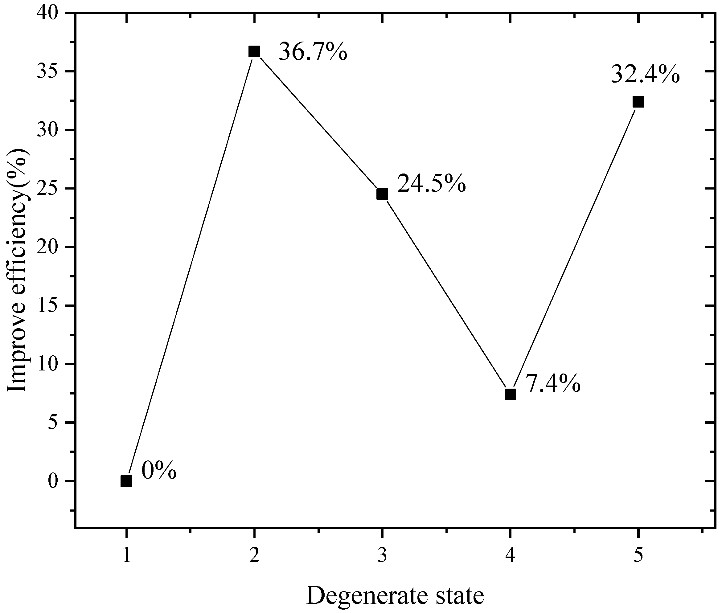
As can be seen from Figure 12, the points added by AK-ARBIS are basically the same as AK-MCS when there is no degradation at the first state. The reason is that no effective information is available at this state. Afterwards, the improved efficiency is 36.7%, 24.5%, 7.4% and 32.4%, respectively. Although the efficiency of some states is not high, the AK-ARBIS method is still more efficient than the AK-MCS method on the whole.

4.2. A Steering Mechanism

Figure 13 shows a steering mechanism, where the length of the left control arm (1) and the right control arm (4) are L b , and the length of the left steering link rod (2) and the right steering link rod (3) are L t . The length of the lower axle is W , and the distance between the lower axle and rack axle (5) is H . The input variable is set as the transverse distance D of the rack axle (5), and the corresponding output variable is the angle η d between the left control arm (1) and the horizontal line. Then the kinematic equation of the steering mechanism considering the clearance can be obtained.
L b cos η 1 + L t cos η 2 + D W / 2 + X 1 X 2 = 0 L b sin η 1 L t sin η 2 H + Y 1 Y 2 = 0
The actual motion output equation can be obtained by eliminating η 2
η 1 = 2 arctan E E 2 4 C F 2 C
where
C = L b 2 + A 2 + B 2 L s 2 2 A L b E = 4 B L b F = 2 A L b + A 2 + B 2 + L b 2 L s 2 A = X 1 X 2 W / 2 D B = Y 1 Y 2 H
In Equation (23), L b , L t , W , H and clearance circle C i X i , Y i are taken as random variables, and the specific distributions are shown in Table 3 and Table 4. The failure mode of the steering mechanism is defined as
g ( L b , L b , W , H , X i , Y i ) = Δ η 1 η i d     ( i = 1 , 2 )
It means that the mechanism fails when the difference between the output angle η 1 in the presence of clearance circle and the output angle η i d in the ideal case is greater than the threshold Δ = 0.087   rad .
Table 5 shows the failure probability and the corresponding C.O.V value calculated by MCS, AK-MCS and the proposed AK-ARBIS method. As can be seen, when compared with the MCS method, the AK-ARBIS method and AK-MCS method have extremely high accuracy (the error is controlled within 5%), but the AK-ARBIS method saves 49.49% of the calculation cost compared to the AK-MCS method.
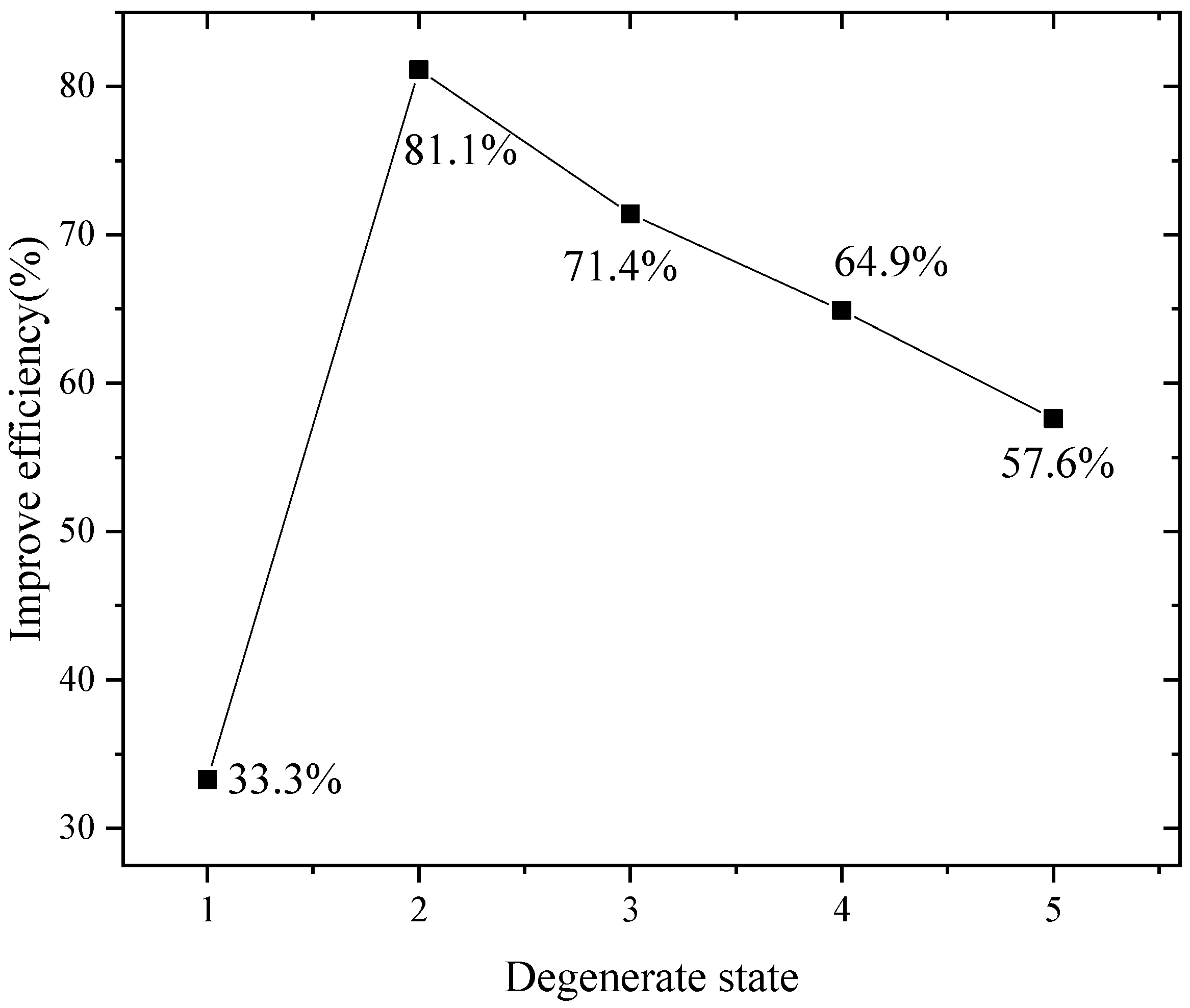
It can be seen from Figure 14, the improved efficiency was 33.3%, 81.1%, 71.4%, 64.9% and 57.6%, respectively. The number of points in different states by the AK-ARBIS is far less than the AK-MCS, especially in later states. Combined with the analysis of the two mechanism examples, the improved efficiency is not very high in the initial state due to less effective information that can be inherited. But with the degradation, there is a significant improvement, which verifies the efficiency of the new method.

5. Application of Adjusting Mechanism

5.1. Random Variables

The pins are the key component that connects the entire mechanism, and their uncertainties affect the kinematic and dynamic characteristics transferred between components. Therefore, the friction coefficients f 1 , f 2 and the radius sizes r 1 , r 2 at the two pins are considered as random variables. In addition, the pressure data in the actual working conditions are uncertain, and then the load moment M in the end of the scale blade is considered as a random variable. In engineering, the values of pin radii are all bounded, so reasonable normal random variable parameters are selected. The friction coefficient between each transmission component will fluctuate and is difficult to determine, so it is treated as uniform distribution. In this work, it is assumed that the random variables considered are independent of each other, and the specific distributions are shown in Table 6.
During the degradation, the radii of the pins are still assumed to follow truncated normal distribution. The calculation method of mechanism wear proposed in Section 2 can be used to predict the degenerate performance under different wear states. In order to facilitate the verification of the sequential reliability analysis, the specific wear depth values in five states are selected from their degenerate tracks in Table 7. And the distribution information of the radii is given.

5.2. Failure Mode

According to the motion characteristics of the adjusting mechanism, the motion accuracy is considered as the failure mode. Suppose that the actually achieved angle is ξ , and the angle under the ideal condition without wear is ξ * . Then the actual angle difference generated is given as ξ ξ * . It is assumed that the tolerance angle error for the adjusting mechanism is Δ , then, the failure mode of motion accuracy is defined as
g ( X ) = Δ ξ ξ *
where ξ is a function of random variable X , which can be obtained by dynamic simulation analysis. Unlike the previous two numerical examples of mechanisms, this failure mode cannot be expressed explicitly.

5.3. Result of Sequential Reliability Analysis

For the adjusting mechanism, the entire process of sequential reliability analysis is performed by calling the dynamic simulation results in ADAMS and completing the reliability analysis in MATLAB. According to Table 8, the failure probability and the corresponding C.O.V value calculated by AK-MCS and the proposed AK-ARBIS method are given. As can be seen, the AK-ARBIS method and AK-MCS method both have extremely high accuracy (within 5%) in states 4 and 5 when compared with each other as the degenerate progresses. The reason for the large error of states 1, 2 and 3 is that the failure probability is small in the early state of wear degradation, and the candidate sample pool of tradeoff calculation cost does not have a large value. In addition, compared with the AK-MCS method, the AK-ARBIS method reduces the call times for the model of the adjusting mechanism and saves the calculation cost of reliability analysis.
As can be seen from Figure 15, the points added by the AK-MCS and AK-ARBIS method are reduced in each state, and the computational efficiency is improved by 60.0%, 100.0%, 71.4%, 59.5% and 48.9%, respectively. The number of points in these states of AK-ARBIS is far less than that of AK-MCS, which verifies the efficiency of the sequential reliability analysis.
The numerical simulation of clearance wear was carried out for the adjusting mechanism, and the wear depth of corresponding states was obtained, which provided sequential reliability analysis of wear degradation. In this example, the calculation efficiency is improved by constructing multiple Kriging models. The convergence condition is gradually met if the number of the added points does not exceed 100 in each degenerate state, which means that the dynamical simulation is called for less than 100 times. Under the allowable angle error, the failure probability increases gradually with the update of degenerate state. This indicates that the clearance between the pins increases continuously due to wear degradation and affects the motion accuracy of the adjusting mechanism. Therefore, during the service life of mechanical equipment, regularly inspecting and replacing the pins with serious wear is necessary, which provides a new idea for improving the reliability of the mechanism.

6. Conclusions

The main purpose of this paper was to improve the reliability analysis and calculation efficiency of the mechanism with hinge clearance at each state of wear degradation. Due to the extensive uncertainty of the mechanism, the wear degradation of the hinge exacerbates the size of the clearance, which affects the accuracy of its motion. Based on dynamic simulation of the adjusting mechanism, the tracks of wear depth of its hinges were computed. Then, because of the feature of sequential degradation, sequential reliability analysis based on AK-ARBIS was proposed in the standard normal space, which greatly reduced the size of the candidate sample pool. With the inward search of the sphere, the Kriging models were updated and the model information in each degenerate state could be used, which reduced the number of calls to the performance function. The results show that the proposed method is more efficient and accurate than the traditional method through two typical mechanism examples and the application of the adjusting mechanism. In the engineering field, this has practical guiding significance for the preventive maintenance of mechanical equipment.
Furthermore, there is a disadvantage that the Kriging model needs to be constructed repeatedly for each degenerate state. Predicting the response under various wear states by using only one Kriging model will be investigated in future work.

Author Contributions

Writing—original draft preparation, H.H.; writing—review and editing, P.W.; investigation and simulation, H.H. and H.Z. All authors have read and agreed to the published version of the manuscript.

Funding

This research was funded by the National Natural Science Foundation of China (Grant No: 51975473) and the Aviation Science Foundation for the Aviation Key Laboratory of Science and Technology on Life-support Technology (Grant No. 201929053001).

Institutional Review Board Statement

Not applicable.

Informed Consent Statement

Not applicable.

Data Availability Statement

The data presented in the study are available on request from the corresponding author.

Conflicts of Interest

The authors declare no conflict of interest.

References

  1. Arif, I.; Masud, J.; Shah, S. Computational Analysis of Integrated Engine Exhaust Nozzle on a Supersonic Fighter Aircraft. J. Appl. Fluid Mech. 2018, 11, 1511–1520. [Google Scholar] [CrossRef]
  2. Sloan, B.; Wang, J.; Spence, S.; Raghunathan, S.; Riordan, D. Aerodynamic performance of a bypass engine with fan nozzle exit area change by warped chevrons. Proc. Inst. Mech. Eng. Part G J. Aerosp. Eng. 2009, 224, 731–743. [Google Scholar] [CrossRef]
  3. Flores, P. A parametric study on the dynamic response of planar multibody systems with multiple clearance joints. Nonlinear Dyn. 2010, 61, 633–653. [Google Scholar] [CrossRef]
  4. Zhu, A.B.; He, S.L.; Zou, C.; Chen, W. The effect analysis of contact stiffness on wear of clearance joint. J. Tribol. 2017, 139, 031403. [Google Scholar] [CrossRef]
  5. Lai, X.M.; Lai, Q.F.; Huang, H.; Wang, C.; Yang, J.H.; Zhang, Y. New approach to assess and rank the impact of revolute joint wear on the kinematic accuracy in the low-velocity planar mechanism. Adv. Eng. Softw. 2016, 102, 71–82. [Google Scholar] [CrossRef]
  6. Sun, Z.C.; Yu, T.X.; Pang, H.; Song, B.F. Failure mechanism and reliability analysis of the rear cargo door lock of transport aircraft. Eng. Fail. Anal. 2021, 122, 105182. [Google Scholar] [CrossRef]
  7. Lai, X.M.; He, H.; Lai, Q.F.; Wang, C.; Yang, J.H.; Zhang, Y.; Fang, H.Y.; Liao, S.R. Computational prediction and experimental validation of revolute joint clearance wear in the low-velocity planar mechanism. Mech. Syst. Signal Process. 2017, 85, 963–976. [Google Scholar] [CrossRef]
  8. Zhang, J.F.; Du, X.P. Time-dependent reliability analysis for function generation mechanisms with random joint clearances. Mech. Mach. Theory 2015, 92, 184–199. [Google Scholar] [CrossRef]
  9. Bai, Z.F.; Zhao, Y.; Chen, J. Dynamics analysis of planar mechanical system considering revolute clearance joint wear. Tribol. Int. 2013, 64, 85–95. [Google Scholar] [CrossRef]
  10. Geng, X.Y.; Li, M.; Liu, Y.F.; Zheng, W.; Zhao, Z.J. Non-probabilistic kinematic reliability analysis of planar mechanisms with non-uniform revolute clearance joints. Mech. Mach. Theory 2019, 140, 413–433. [Google Scholar] [CrossRef]
  11. Li, J.L.; Huang, H.Z.; Yan, S.Z.; Yang, Y.Q. Kinematic accuracy and dynamic performance of a simple planar space deployable mechanism with joint clearance considering parameter uncertainty. Acta Astronaut. 2017, 136, 34–45. [Google Scholar] [CrossRef]
  12. Tian, Q.; Flores, P.; Lankarani, H.M. A comprehensive survey of the analytical, numerical and experimental methodologies for dynamics of multibody mechanical systems with clearance or imperfect joints. Mech. Mach. Theory 2018, 122, 1–57. [Google Scholar] [CrossRef]
  13. Wu, J.N.; Yan, S.Z.; Li, J.N.; Gu, Y.X. Mechanism reliability of bistable compliant mechanisms considering degradation and uncertainties: Modeling and evaluation method. Appl. Math. Model. 2016, 40, 10377–10388. [Google Scholar] [CrossRef] [Green Version]
  14. Ye, Z.-S.; Xie, M. Stochastic modelling and analysis of degradation for highly reliable products. Appl. Stoch. Models Bus. Ind. 2015, 31, 16–32. [Google Scholar] [CrossRef]
  15. Wu, J.N.; Yan, S.Z.; Zuo, M.J. Evaluating the reliability of multi-body mechanisms: A method considering the uncertainties of dynamic performance. Reliab. Eng. Syst. Saf. 2016, 149, 96–106. [Google Scholar] [CrossRef]
  16. Li, X.Y.; Chen, W.B.; Kang, R. Performance margin-based reliability analysis for aircraft lock mechanism considering multi-source uncertainties and wear. Reliab. Eng. Syst. Saf. 2021, 205, 107234. [Google Scholar] [CrossRef]
  17. Zhuang, X.C.; Yu, T.X.; Shen, L.J.; Sun, Z.C.; Guo, B.Z. Time-varying dependence research on wear of revolute joints and reliability evaluation of a lock mechanism. Eng. Fail. Anal. 2019, 96, 543–561. [Google Scholar] [CrossRef]
  18. Lv, Z.Y.; Lu, Z.Z.; Wang, P. A new learning function for Kriging and its applications to solve reliability problems in engineering. Comput. Math. Appl. 2015, 70, 1182–1197. [Google Scholar] [CrossRef]
  19. Zhang, L.G.; Lu, Z.Z.; Wang, P. Efficient structural reliability analysis method based on advanced Kriging model. Appl. Math. Model. 2015, 39, 781–793. [Google Scholar] [CrossRef]
  20. Echard, B.; Gayton, N.; Lemaire, M. AK-MCS: An active learning reliability method combining Kriging and Monte Carlo Simulation. Struct. Saf. 2011, 33, 145–154. [Google Scholar] [CrossRef]
  21. Zheng, P.J.; Wang, C.M.; Zong, Z.H.; Wang, L.Q. A new active learning method based on the learning function U of the AK-MCS reliability analysis method. Eng. Struct. 2017, 148, 185–194. [Google Scholar] [CrossRef]
  22. Hu, Z.; Mahadevan, S. A Single-Loop Kriging Surrogate Modeling for Time-Dependent Reliability Analysis. J. Mech. Des. 2016, 138, 061406. [Google Scholar] [CrossRef]
  23. Echard, B.; Gayton, N.; Lemaire, M.; Relun, N. A combined Importance Sampling and Kriging reliability method for small failure probabilities with time-demanding numerical models. Reliab. Eng. Syst. Saf. 2013, 111, 232–240. [Google Scholar] [CrossRef]
  24. Yun, W.Y.; Lu, Z.Z.; Jiang, X. An efficient reliability analysis method combining adaptive Kriging and modified importance sampling for small failure probability. Struct. Multidiscip. Optim. 2018, 58, 1383–1393. [Google Scholar] [CrossRef]
  25. Huang, X.X.; Chen, J.Q.; Zhu, H.P. Assessing small failure probabilities by AK–SS: An active learning method combining Kriging and Subset Simulation. Struct. Saf. 2016, 59, 86–95. [Google Scholar] [CrossRef]
  26. Ling, C.Y.; Lu, Z.Z.; Feng, K.X.; Zhang, X.B. A coupled subset simulation and active learning kriging reliability analysis method for rare failure events. Struct. Multidiscip. Optim. 2019, 60, 2325–2341. [Google Scholar] [CrossRef]
  27. Liu, H.; He, X.D.; Wang, P.; Lu, Z.Z.; Yue, Z.F. Time-dependent reliability analysis method based on ARBIS and Kriging surrogate model. Eng. Comput. 2022, 1–14. [Google Scholar] [CrossRef]
  28. Wang, P.; Zhou, H.Y.; Hu, H.H.; Zhang, Z.; Li, H.H. A novel method for reliability analysis with interval parameters based on active learning Kriging and adaptive radial-based importance sampling. Int. J. Numer. Methods Eng. 2022, 123, 3264–3284. [Google Scholar] [CrossRef]
  29. Yun, W.Y.; Lu, Z.Z.; Jiang, X.; Zhang, L.G.; He, P.F. AK-ARBIS: An improved AK-MCS based on the adaptive radial-based importance sampling for small failure probability. Struct. Saf. 2020, 82, 101891. [Google Scholar] [CrossRef]
  30. Depina, I.; Le, T.M.H.; Fenton, G.; Eiksund, G. Reliability analysis with Metamodel Line Sampling. Struct. Saf. 2016, 60, 1–15. [Google Scholar] [CrossRef]
  31. Dumas, A.; Echard, B.; Gayton, N.; Rochat, O.; Dantan, J.Y.; Van der Veen, S. AK-ILS: An Active learning method based on Kriging for the Inspection of Large Surfaces. Precis. Eng. 2013, 37, 1–9. [Google Scholar] [CrossRef] [Green Version]
  32. Su, M.J.; Xue, G.F.; Wang, D.Y.; Zhang, Y.S.; Zhu, Y. A novel active learning reliability method combining adaptive Kriging and spherical decomposition-MCS (AK-SDMCS) for small failure probabilities. Struct. Multidiscip. Optim. 2020, 62, 3165–3187. [Google Scholar] [CrossRef]
  33. Bichon, B.J.; Eldred, M.S.; Swiler, L.P.; Mahadevan, S.; McFarland, J.M. Efficient Global Reliability Analysis for Nonlinear Implicit Performance Functions. Aiaa J. 2008, 46, 2459–2468. [Google Scholar] [CrossRef]
  34. Wang, Z.Q.; Wang, P.F. A Maximum Confidence Enhancement Based Sequential Sampling Scheme for Simulation-Based Design. J. Mech. Des. 2014, 136, 021006. [Google Scholar] [CrossRef]
  35. Sun, Z.L.; Wang, J.; Li, R.; Tong, C. LIF: A new Kriging based learning function and its application to structural reliability analysis. Reliab. Eng. Syst. Saf. 2017, 157, 152–165. [Google Scholar] [CrossRef]
  36. Jiang, C.; Qiu, H.B.; Yang, Z.; Chen, L.M.; Gao, L.; Li, P.G. A general failure-pursuing sampling framework for surrogate-based reliability analysis. Reliab. Eng. Syst. Saf. 2019, 183, 47–59. [Google Scholar] [CrossRef]
  37. Murray, R. Remarks on a Multivariate Transformation. Ann. Math. Stat. 1952, 23, 470–472. [Google Scholar] [CrossRef]
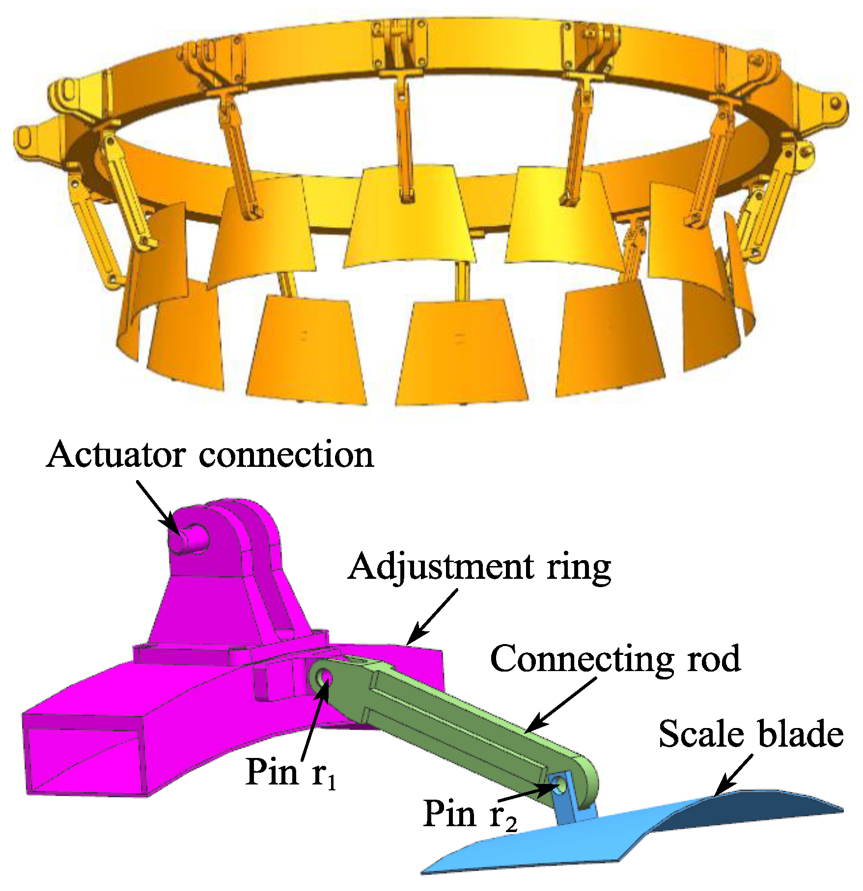
Figure 1. Full model and simplified model of adjusting mechanism.
Machines 10 00613 g001
Figure 2. Contact force and contact surface of hinge clearance.
Machines 10 00613 g002
Figure 3. Variation curve of scale blade angle with time.
Machines 10 00613 g003
Figure 4. Normal pressure diagram at different pins.
Machines 10 00613 g004
Figure 5. Calculation of equivalent contact area when pin and bushing have contact.
Machines 10 00613 g005
Figure 6. Wear depth of different pins of a single rotation cycle.
Machines 10 00613 g006
Figure 7. The accumulated wear depth corresponding to different motion cycles.
Machines 10 00613 g007
Figure 8. Transformation from the degenerate sample space to the standard normal space.
Machines 10 00613 g008
Figure 9. Schematic diagram of AK-ARBIS.
Machines 10 00613 g009
Figure 10. Schematic diagram of Kriging model in different degenerate states.
Machines 10 00613 g010
Figure 11. Schematic diagram of four-bar linkage.
Machines 10 00613 g011
Figure 12. Improve efficiency by increasing the number of points.
Machines 10 00613 g012
Figure 13. Schematic diagram of steering mechanism.
Machines 10 00613 g013
Figure 14. Improve efficiency by increasing the number of points.
Machines 10 00613 g014
Figure 15. Improve efficiency by increasing the number of points.
Machines 10 00613 g015
Table 1. Distributions of random variables.
VariableDistribution Radius   of   Clearance   Circle   r c i
C i X i , Y i 2D-uniform with a circle0.0180.0190.0200.0210.022
Table 2. Calculation results of a four-bar linkage mechanism.
MethodsStates N c a l l P f C.O.V (%)
MCS
( 1 × 10 6 )
State 1 1 × 10 6 6.94 × 10 - 4 3.7946
State 2 1 × 10 6 0.00152.5801
State 3 1 × 10 6 0.00271.9219
State 4 1 × 10 6 0.00441.5042
State 5 1 × 10 6 0.00671.2176
AK-MCS
( 1 × 10 6 )
State 150 + 115 6.20 × 10 4 4.0149
State 250 + 1800.00152.5801
State 350 + 2450.00271.9219
State 450 + 2960.00431.5217
State 550 + 4440.00651.2363
AK-ARBIS
( 1 × 10 6 )
State 150 + 122 6.48 × 10 4 3.9271
State 250 + 1140.00152.5801
State 350 + 1850.00261.9586
State 450 + 2740.00431.5217
State 550 + 3000.00651.2363
Table 3. Distributions of random variables of size.
VariableDistributionMean (mm)Standard Deviation (mm)
L b Normal1110.1
L t Normal283.50.1
W Normal650.240.1
H Normal83.50.1
Table 4. Distributions of random variables of clearance circle.
VariableDistribution Radius   of   Clearance   Circle   r c i
C i X i , Y i 2D-uniform with a circle0.00460.00470.00480.00490.0050
Table 5. Calculation results of a steering mechanism.
MethodsStates N c a l l P f C.O.V (%)
MCS
( 1 × 10 5 )
State 1 1 × 10 5 0.01782.3490
State 2 1 × 10 5 0.01982.2249
State 3 1 × 10 5 0.02182.1183
State 4 1 × 10 5 0.02422.0080
State 5 1 × 10 5 0.02661.9129
AK-MCS
( 1 × 10 5 )
State 150 + 1890.01772.3558
State 250 + 1900.01942.2483
State 350 + 1960.02182.1183
State 450 + 2080.02441.9996
State 550 + 2360.02691.9020
AK-ARBIS
( 1 × 10 5 )
State 150 + 1260.01782.3490
State 250 + 360.01912.2662
State 350 + 560.02152.1333
State 450 + 730.02402.0166
State 550 + 1000.02701.8983
Table 6. Distributions of random variables.
VariableDistribution TypeDistribution Parameter 1Distribution Parameter 2
r 1 (mm)Truncated normal2.850.05
r 2 (mm)Truncated normal2.850.05
f 1 Uniform0.010.15
f 2 Uniform0.010.15
M (N·m)Uniform55.9260.92
Table 7. Wear depth and distributions of the radii under degradation.
Wear Cycles
(Different States)
Wear Depth (mm)Radii (Truncated Normal Distribution)
Δ r 1 Δ r 2 Standard Deviation (0.05)
Mean   Value   r 1 Mean   Value   r 2
State 1 (initial clearance)002.852.85
State 2 (3300 cycles)0.00740.01772.85–0.00742.85–0.0177
State 3 (6600 cycles)0.01480.03552.85–0.01482.85–0.0355
State 4 (9900 cycles)0.02210.05292.85–0.02212.85–0.0529
State 5 (13,200 cycles)0.02940.07032.85–0.02942.85–0.0703
Table 8. Calculation results of adjusting mechanism.
MethodsStates N c a l l P f C.O.V (%)
AK-MCS
( 1 × 10 6 )
State 125 + 50.00034.9999
State 225 + 100.00113.0135
State 325 + 210.00351.6873
State 425 + 420.00911.0435
State 525 + 920.02170.6714
AK-ARBIS
( 1 × 10 6 )
State 125 + 20.00054.4710
State 225 + 00.00132.7717
State 325 + 60.00401.5780
State 425 + 170.00881.0613
State 525 + 470.02200.6667
Publisher’s Note: MDPI stays neutral with regard to jurisdictional claims in published maps and institutional affiliations.